Security Trade-Off and Energy Efficiency Analysis in Wireless Sensor Networks

Abstract

With a rapid progress of numerous applications in wireless sensor networks (WSNs), performance evaluation and analysis techniques face new challenges in energy efficiency area in WSN applications. One of the key issues is to perform the security trade-off and energy efficiency analysis. In this paper, the energy analysis module for the QoP-ML (quality of protection modeling language) is proposed by means of which one can analyze the influence of various security levels on the energy consumption of a protocol. Moreover, an advanced communication module is proposed as an extension of the QoP-ML language, which enhances the abilities to analyze complex wireless sensor networks. The case study of WSN deployed on the Jindo Bridge in South Korea was carried out and the lifetime of protocols with various security levels was simulated. The results show that the introduction of various security levels can entail large differences in performance and energy consumption, and hence result in different lifetime. Therefore, the designers of WSN protocols should search for balance between the required lifetime and security level. The introduced QoP-ML extension, along with the AQoPA (automated quality of protection analysis) tool, has been developed to meet the above requirements.

1. Introduction

In today's world we witness a rapid growth of information and communication techniques for wireless sensor networks (WSNs). This progress has created a need for their analysis and performance evaluation. One of the most investigated problems of WSN applications is energy efficiency [1, 2]. In addition, the search for trade-offs between energy effectiveness and security assurance needs to be taken into consideration. Designing secure protocols which satisfy the required performance is an important issue to be solved. The traditional approach assumes that the best way is to apply the strongest possible security mechanisms, which make the system as secure as possible. Unfortunately, such reasoning leads to the overestimation of security measures, which causes an unreasonable increase in system load [3, 4]. Determination of the required quality of protection (QoP) and adjustment of some security measures to meet these concerns (QoP modeling) can be a solution to the above problems.

In the literature, many energy-efficient solutions have been proposed due to the scare battery resources of the sensors, which limits the network lifetime. Many of them concentrate on the MAC and PHY layers (standards [5–7]) and on routing and messaging protocols [8, 9]. However, there exist also application-specific solutions like data reduction (aggregation, compression) and new technologies used for harvesting energy [10].

Energy-efficient solutions are always measured and compared with their predecessors. Measurements can be done either by experiments or simulations. As the first solution is in many cases quite hard to perform the simulation is used instead. There exists many evaluation techniques, such as data or bits flow analysis, the state transition modeling based on Markov chain, and Petri net or model-driven architecture analysis. One can use tools like [11], which is a real-time network emulator, or evaluation platforms like [12]. However, in [13] authors point out that most of classical energy models are generally oversimplified and focus only on RF transceivers ignoring other components, what may result in imprecise evaluation especially when taking into account the cases with heavy workloads on processors and sensors. They propose an event-driven queuing Petri net (QPN) [13] model to simulate the energy consumption behaviors of sensor. The QPN model allows us to evaluate the energy consumption of sensor, transceiver, and processor units including their state transitions.

Besides the energy effectiveness, security is another requirement present among the other requirements in the most of WSN applications. In [10] authors present interdependences between energy-efficient mechanisms and application requirements. Despite the fact the security is listed as one of requirements the interdependence between security and energy effectiveness is not analyzed.

Many modeling languages and tools to analyze the security of cryptographic protocols have been developed. However, the proposed approaches do not consider the topic of trade-off between security and energy efficiency. There exist tools like Scyther [23], Avispa [24], and Proverif [25] which perform a formal, automatic verification of protocol by proving the correctness of specified security requirements or by finding the flaw in the protocol. These tools, however, do not evaluate the performance. Other tools, like UMLSec [26], which deal with the security level of analysed systems are used for software development and fail to include the analysis of communication steps and their impact on system performance and security level.

To the best of the authors’ knowledge, the QoP-ML (quality of protection modeling language) is the only modeling language which allows us to balance security against performance and accomplishes a multilevel analysis of the protocol, extending the possibility of describing the state of a cryptographic set of actions. Every single operation defined by the QoP-ML is characterised by security metrics which evaluate the impact of this operation on overall system security [27]. The QoP-ML was used to simulate cryptographic protocols designed for a wireless sensor network. The correctness of this analysis was positively verified by experiments [28].

The relevant type of operation is a communication process which must be included in the performance analysis of a system. The original communication model of the QoP-ML has a few limitations caused by the use of channels representing the link between each pair of hosts. The first limitation is the impossibility to determine the receiver of the message when many hosts use the same channel. In such a case, the message will be delivered to the first host in the queue of hosts waiting for the message on the channel. The inability to define the sender of the message in order to send back the response is another known limitation.

The main contributions of this paper are summarized as follows.

• (i)

We propose an extension of the QoP-ML which allows us to accomplish a complex network analysis as part of protocol performance analysis. Furthermore, we introduce an advanced communication module, which during the analysis takes into account the following elements: network topology, routing, and packet filtering. This new module removes all the above-listed limitations of the QoP-ML.

(ii)

We propose an energy efficiency module by means of which one can analyze the influence of given operations on energy consumption and system lifetime.

(iii)

The two modules introduced in this paper are implemented in the Automatic Quality of Protection Analysis Tool (AQoPA). The AQoPA performs automatic evaluation and optimization of complex system models created in QoP-ML.

(iv)

We present a case study of energy efficiency analysis and security trade-offs for a complex wireless sensor network. Using this example, we want to present a method to find a trade-off between security and energy efficiency. The case study is based on an existing WSN deployed on the Jindo Bridge in South Korea [29].

The remaining part of this paper is organized as follows. Section 2 contains the comparison of the QoP-ML to other solutions used to analyze the security of protocols and their influence on performance. Section 3 describes briefly the elements of the QoP-ML language. In Section 4, a new communication model and its features and structures are described. In Section 5, the energy analysis module is explained, and in Section 6, we present a case study which uses the new functionality of the introduced communication model. Last section, Section 7, concludes the paper.

2. Related Work

All services provided by information systems of any nature (e.g., WSN, cloud, etc.) should be guaranteed by the provider and formalized in contracts. This is achieved by the SLA (service-level agreement) which defines a process of continuous monitoring and maintaining the quality of service (QoS) on the agreed level. In particular, SLA specifies the conditions (QoS parameters) under which service is delivered [30]. Conditions can be very different depending on the type of service. For example, in case of call center, a condition can specify average time it takes for a call to be answered by the service desk. On the other hand, data storage companies can specify availability as one of conditions which is the ratio of the total time a system is capable of being used during a given interval of time to the length of the interval.

The ideal system ensures the quality of service on the highest level. However, it involves high costs and when the expense of mechanisms to provide QoS is justified the provider negotiates QoS parameters (conditions) with clients. The result of negotiations is the agreed level of quality of service to be guaranteed by the provider.

The quality of service term can have various meanings [31]. Usually it is referred to the overall performance of computer network. In RFC 2386 [32], QoS has been defined as a set of service requirements to be fulfilled when transmitting a stream of packets from source to destination. However, in the literature the requirements of QoS are defined from two perspectives: mentioned network QoS and application specific QoS [31, 33]. In the application communities, QoS generally refers to the quality as perceived by the user/application.

Assuming such broad interpretation of QoS term, one can find a subset of conditions that refer directly to the security. These can be confidentiality, authentication, integrity, availability, and many other conditions. Most of them can be associated with network QoS but some can be also application specific. For example, availability condition in network QoS can be understood as successful transmission of data from source to destination (with additional time requirements), while an application can add its derived requirements like coverage [34] when application requires whole monitored area to be covered.

Extraction of the subset of conditions that refer directly to the security gives possibility to measure the quality of protection (QoP) in analyzed system. In such case, QoP is understood as the part of QoS. Some of the conditions can overlap; for example, performance requirements (e.g., transmission time, protocol execution time, energy efficiency, and lifetime) which are strictly connected with QoS have great impact on the availability requirement which belongs to QoP requirements.

Introduction of QoP term allows us to concentrate on security requirements and extends the SLA negotiations of requirements by adding new variable (QoP derived from QoS) to previous two: QoS (as performance) and costs.

In the literature, the security trade-off is based on the quality of protection (QoP) models. These models were created for different purposes and have different features and limitations. The related research in this area is presented below.

Lindskog attempts to extend security layers in a few quality of service (QoS) architectures [17]. Unfortunately, the descriptions of the methods are limited to the confidentiality of data and based on different configurations of the cryptographic modules. Ong et al. in [19] present the QoP mechanisms which define security levels depending on security parameters. These parameters are as follows: key length, block length, and the contents of an encrypted block of data. Schneck and Schwan [21] propose an adaptable protocol concentrating on authentication. By means of this protocol, one can change the version of the authentication protocol, which finally changes the parameters of the asymmetric and symmetric ciphers. Sun and Kumar [22] create the QoP models based on vulnerability analysis which is represented by attack trees. The leaves of the trees are described by means of the special metrics of security. These metrics are used for describing individual characteristics of the attack. In the article [15], Ksiezopolski and Kotulski introduce mechanisms for adaptable security which can be used for all security services. In this model, the quality of protection depends on the risk level of the analysed processes. Luo et al. [18] provide the quality of protection analysis for the IP multimedia systems (IMS). This approach presents the IMS performance evaluation using the queuing networks and stochastic Petri nets. In the paper [14], Agarwal and Wang present the performance impact of security protocols in wireless LANs with IP mobility and introduce the QoP model to quantify the benefits of security policies and demonstrate the relationship between the QoS and the QoP. LeMay et al. [16] create an adversary-driven, state-based system security evaluation, a method which evaluates quantitatively the strength of system security. In the paper [20], Petriu et al. present the performance analysis of security aspects in the UML models. This approach takes as an input the UML model of the system designed by the UMLsec extension [26] of the UML modeling language. This UML model is annotated with the standard UML profile for schedulability, performance, and time and then analysed for performance. In the article [35], Ksiezopolski introduces the quality of protection modeling language which provides the modeling language for making abstraction of cryptographic protocols with emphasis on the details concerning the quality of protection. Table 1 demonstrates the approach presented in this paper as compared to the existing methodologies. These approaches can be characterised by the following main attributes.

• (i)

Quantitative assessment (QA) refers to the quantitative assessment of the estimated quality of protection of the system.

(ii)

Executability (E) specifies the possibility of the implementation of an automated tool able to perform the QoP evaluation.

(iii)

Consistency (Con) is the ability to model the system maintaining its states and communication steps consistency.

(iv)

Performance evaluation (PE) gives the possibility of performance evaluation of the analysed system.

(v)

Energy evaluation (EE) gives the possibility of energy efficiency evaluation of the analysed system.

(vi)

Holistic (H) approach gives the possibility of the evaluation of all security attributes.

(vii)

Completeness (Com) is the possibility of the representation of all security mechanisms. This attribute is provided for all models.

Table 1

The characterisation of the QoP models.

	QA	E	Con	EE	H	Com	PE
Agarwal and Wang [14]	✓	—	—	—	✓	✓	✓
Ksiezopolski and Kotulski [15]	✓	✓	—	—	✓	✓	—
LeMay et al. [16]	—	✓	✓	—	—	—	—
Lindskog [17]	✓	—	✓	—	—	—	✓
Luo et al. [18]	✓	—	—	—	✓	✓	✓
Ong et al. [19]	✓	—	—	—	—	—	—
Petriu et al. [20]	—	✓	✓	—	—	✓	✓
Schneck and Schwan [21]	✓	—	✓	—	—	—	✓
Sun and Kumar [22]	✓	—	—	—	—	—	—
QoP-ML	✓	✓	✓	✓	✓	✓	✓

One can notice that only QoP-ML can be used for finding a trade-off between security (QA) and performance (PE) including energy efficiency evaluation (EE) of the system which is modeled in a formal way with communication steps consistency (Con). By means of QoP-ML, one can evaluate all security attributes (H) and abstract all security mechanisms which protect the system (C). Additionally, the QoP-ML approach is supported by the tool (E) required for the analysis of complex systems.

3. QoP-ML

In the paper [35], Ksiezopolski introduces the quality of protection modeling language, which provides the modeling language for making abstraction of cryptographic protocols with emphasis on the details concerning the quality of protection. The intended use of the QoP-ML is to represent a series of steps described as a cryptographic protocol. The QoP-ML has introduced a multilevel protocol analysis which extends the possibility of describing the state of a cryptographic protocol.

3.1. General View

Structures used in the QoP-ML represent a high level of abstraction which allows us to focus on the quality of protection analysis. The QoP-ML consists of processes, functions, message channels, variables, and QoP metrics. Processes are global objects grouped into the main process, which represents a single computer (host). A process specifies behaviour, functions represent a single operation or a group of operations, and channels define the environment in which a process is executed.

The QoP metrics define the influence of functions and channels on the quality of protection. In the paper [35], the syntax, semantics, and algorithms of the QoP-ML are presented.

3.2. Data Types

In the QoP-ML, an infinite set of variables is used for describing communication channels, processes, and functions. Variables are used to store information about the system or a specific process. The QoP-ML is an abstract modeling language, so there are no special data types, sizes, or value ranges. Variables do not have to be declared before they are used. They are automatically declared when they are used for the first time.

The scope of variables declared inside a high hierarchy process (host) is global for all processes defined inside a host.

3.3. Functions

System behaviour is changed by functions which modify the states of variables and pass objects by communication channels. When defining a function, one has to set the arguments of this function which describe two types of factors. Functional parameters written in round brackets are necessary for the execution of a function while additional parameters written in square brackets influence the system quality of protection. The names of arguments are unrestricted.

3.4. Equation Rules

Equation rules play an important role in the quality of protection protocol analysis. Equation rules for a specific protocol consist of a set of equations asserting the equality of function calls. For instance, the decryption of the encrypted data with the same key is equal to the encrypted data.

3.5. Process Types

Elements describing system behaviour (functions, message passing) are grouped into processes which constitute the main objects in the QoP-ML. In a real system, processes are executed and maintained by a single computer. In the QoP-ML, sets of processes are grouped into a higher hierarchy process named host.

All variables used in a high hierarchy process (host) have a global scope for all processes grouped inside this structure. Normally, variables used inside a host process cannot be applied for another high hierarchy process. This operation is possible only when a variable is sent by a communication channel.

3.6. Message Passing

Communication between processes is modeled by means of channels which are used to pass messages between hosts and processes in the FIFO (first-in first-out) order. Before a message is sent, a channel must be declared because its declaration contains a buffer size and other channel's characteristics. When channels are declared with a nonzero buffer size, communication is asynchronous, whereas a buffer size equal to zero stands for synchronous communication. In synchronous communication, the sender transmits data through a synchronous channel only if the receiver listens to this channel. When the size of the buffer channel equals at least 1, a message can be sent through this channel even if no one is listening on this channel. This message will be transmitted to the receiver when the listening process in this channel is executed.

3.7. Security Metrics

System behavior, which is formally described by a cryptographic protocol, can be modeled by the proposed QoP-ML. One of the main aims of this language is to abstract the quality of protection of a particular version of the analysed cryptographic protocol. In the QoP-ML, the influence of system protection is represented by means of functions. While declaring a function, the quality of protection parameters is defined and the details about this function are described. These factors do not influence the flow of a protocol, but they are crucial for the quality of protection analysis. During such an analysis, functions’ QoP parameters are combined with the next structure of the QoP-ML, that is, security metrics. In this structure, one can abstract functions’ time performance, their influence on the security attributes required for a cryptographic protocol, or other factors important during the QoP analysis.

4. Advanced Network Analysis Module

The introduction of new network analysis module eliminates the weaknesses of the original one (from QoP-ML). Briefly mentioning, the first weakness is the impossibility to determine the receiver of the message when many hosts use the same channel while the second one is the inability to define the sender of the message in order to send back the response.

Removal of the limitations enumerated above requires the creation of new mechanisms and structures in the QoP-ML model. In this section, we describe three new mechanisms: topology, routing, and packet filtering. In addition, we introduce a methodology which provides time analysis of communication steps in a network. Depending on the selected path in a network, the time of delivering a message from the sender to the receiver can vary. The model allows to determine the characteristics of a channel and calculate the time of transmission.

The syntax of all structures introduced in this paper is presented in Supplementary Material available online at http://dx.doi.org/10.1155/2015/943475 using the BNF (Backus-Naur form) [36] standard.

4.1. Topology

A topology is defined by a graph where vertices are hosts and edges are connections between them. All existing connections must be defined and have a weight representing the quality of connection (the lower the weight, the better the quality). A special type of connection is a link between a host and a medium used for broadcasting messages. This connection does not have the quality parameter.

A topology is defined in the topology structure (from line 16 to line 32 in Listing 1) which is a part of the communication structure (see lines from 1 to 34 in Listing 1). The aim of the communication structure is to describe the communication characteristics of mediums (channels). It includes the definition of topology and default topology parameters for all mediums. The communication structure can be located in two places. First, it can be one of the main structures (like hosts, functions, etc.) and affect the whole model and all versions. Secondly, the structure can be placed in the version structure after the run section. In such a case, it affects only the selected version. If the element of the communication structure (e.g., a topology) for a given medium is defined in the version structure, it overrides the main communication structure (i.e., the topology is determined on the basis of the version communication structure only).

Listing 1: An example of a topology definition connected with channel_name tag.

( $$\mathit{1}$$ )     communication  {

( $$\mathit{2}$$ )

( $$\mathit{3}$$ )      medium[cable]  {

( $$\mathit{4}$$ )      default_q  =  0.1;

( $$\mathit{5}$$ )      default_time  =  1 ms;

( $$\mathit{6}$$ )

( $$\mathit{7}$$ )      topology  {

( $$\mathit{8}$$ )       Gateway  ->  Sensor[0];

( $$\mathit{9}$$ )      }

( $$\mathit{10}$$ )   }

(11)

(12)    medium[air_channel]  {

(13)    default_q  =  1;

(14)    default_time  =  18 ms;

(15)

(16)    topology  {

(17)     Sink  <->  Gateway  :  t  =  wsn_time[ms];

(18)

(19)     Sensor  ->  *  :  time  =  17 ms;

( $$\mathit{20}$$ )

( $$\mathit{21}$$ )    Sensor[0]  ->  Gateway,  time  =  5 ms;

( $$\mathit{22}$$ )    Sensor[0]  <-  Gateway  :  q  =  2.5,  time  =  5 ms;

( $$\mathit{23}$$ )    Sensor[1]  <-  Sensor[2]  :  q  =  3.5,  time  =  5 ms;

( $$\mathit{24}$$ )

( $$\mathit{25}$$ )    Sensor[2:5]  ->  Sensor[3];

( $$\mathit{26}$$ )    Sensor[2:]  ->  Sensor[4]  :  time  =  15 ms;

( $$\mathit{27}$$ )    Sensor[:2]  ->  Sensor[5]  :  q  =  3.5,  time  =  15 ms;

( $$\mathit{28}$$ )

( $$\mathit{29}$$ )    Sensor  ->  Sensor[i  +  1]  :  q  =  2;

( $$\mathit{30}$$ )    Sensor[0:5]  <-  Sensor[i  −  2];

( $$\mathit{31}$$ )    Sensor[4:]  <-  Sensor[i  −  3];

( $$\mathit{32}$$ )   }

( $$\mathit{33}$$ )   }

( $$\mathit{34}$$ )  }

4.1.1. Connections Definition

A topology consists of rules which define connections between hosts or between a host and a medium (used for broadcast). A rule has two sets of hosts (left and right), a direction, and, optionally, after the colon, the connection-specific values of parameters. There are three types of direction:

• (1)

A → B, the connection is created from host A to B;

(2)

A ← B, the connection is created from host B to A;

(3)

A ↔ B, the connection is created in both ways.

There are three possible ways of declaring the left set of hosts, all of which are presented in Listing 1.

• (1)

The first way (without indices) includes all hosts with a given name. In Listing 1, they are the rules in lines number 17 and 29. These rules can be used in the main communication structure since the structure does not specify the index of the host.

(2)

The second way (with one index in square brackets) selects only one host, the one with a given index. In Listing 1, they are the rules in lines number 21, 22, and 23.

(3)

The third way (with indices and a colon in square brackets) selects the range of hosts with indices larger than or equal to the first index and lower than or equal to the second index. If the first index is not specified, zero is used, and if the second index is not specified, the number of all hosts with a given name is chosen. The examples are the rules in lines 25, 26, 27, 30, and 31 in Listing 1.

Besides the three methods described above, one can use two additional ways to declare the right set of hosts.

• (1)

The hosts can be specified with a special i index and its modified (increased or decreased) value. In such a case, the hosts with indices shifted by a given value (modification of i) in relation to all hosts from the left set are selected. The example rules are in lines number 29, 30, and 31 in Listing 1. The first rule (line number 29) defines the links between all Sensors and their next neighbours (forming a line) while the second one (line number 30) defines the links between Sensors with indices 0, 1, 2, 3, 4, and 5 and their second predecessor. The last rule (line number 31) creates the link between Sensors with an index larger than or equal to 4 and their third predecessors. When a host does not have a selected neighbour, the link is not created. This type of rule can be used only in the version structure when indices are used on the left side.

(2)

The hosts can be replaced with a star sign (*) which represents a medium. In this case, the quality parameter is not defined and the direction can only be right (from the left hosts to the medium). This type of rule is used to define the parameters for broadcasting a message. The example rule is in line number 19 in Listing 1.

4.1.2. Quality of Connections

Each connection in a topology can be parameterized. Parameters are used to perform the analysis of communication steps. Each parameter can have a default value. To define a default value, one has to precede its name with default_ and place it in the medium structure (lines number 13 and 14 in Listing 1). When a parameter is not defined for a particular connection in a topology, the default value is used.

There is one required parameter q (e.g., numbers 22 and 23 in Listing 1) which represents the quality (weight) of a connection between hosts (the lower the value, the better the quality). The quality parameter is used by the routing algorithm to find the best route between two hosts in multihop communication. It is the resultant value of the environmental factors (e.g., distance, barriers, etc.). This parameter can either be defined statically or estimated dynamically by a defined algorithm. We do not consider the algorithm determining the quality because the QoP-ML is the modeling language not only for WSNs, but also for other systems and protocols. Therefore, algorithms may be entirely different.

4.1.3. Transmission Time

Another important factor in the communication analysis is the time analysis which introduces the time parameter. The proposed parameter represents the time of data transmission between hosts or between a host and a medium (used for broadcast). An example of a definition of a default transmission time is in line number 14 in Listing 1, while a definition of time for a specific connection can be found, for example, in lines number 21, 22, or 23. Its value can be specified as

• (i)

a constant or random number from a specified range in seconds or milliseconds (e.g., line number 19 in Listing 1);

(ii)

a value depending on the size of data: mspb, mspB, kbps, and mbps (a constant or random value from a specified range per bit or byte);

(iii)

a constant or random value from a specified range in seconds or milliseconds per each block of data (e.g., 100 ms per each 16 bytes);

(iv)

the result of an algorithm (e.g., line number 17 in Listing 1) in seconds or milliseconds (algorithms are discussed further in this section).

Depending on the number of receivers, the communication time can vary. The main rules are presented below.

• (i)

When a message is sent to one receiver, the time of communication is equal to the result of the time parameter. The time of the sender and the receiver is increased with the result time.

(ii)

When a message is sent to zero receivers (no one is waiting for a message), the time of communication is equal to the result of the time parameter between a host and a medium (broadcast time). Only the time of the sender is increased.

(iii)

When a message is sent to many receivers, the time of communication can be different for all hosts. The time of sending is equal to the result of the time parameter between the sender and the medium (broadcast time). The sender's time is increased with this value. The time of receiving for each receiver is equal to the maximum value of the time of sending and the result of the time parameter between the sender and the given receiver. As the times of communication between the sender and different receivers can vary, the times of receiving can differ as well.

The easiest way to determine the transmission time in a medium is to take its bandwidth. However, this measure is inaccurate in many cases. In order to define the transmission times more precisely, we introduced the algorithms structure, which provides the possibility of adding nonlinear values of metrics.

An example of an algorithm is presented in Listing 2. It calculates the transmission time between two TelosB motes [28]. The time of transmission is equal to constant 18 ms plus 0.12 ms per each byte. The while loop is used to handle messages with payload larger than 110 bytes, which is the maximal payload size in ZigBee assuming that header has 17 bytes size (the maximal size of packet is 127 bytes) [37]. When the maximal size is exceeded, payload is divided into many packets with a 110 bytes payload size.

Listing 2: An example of an algorithm for the communication time.

( $$\mathit{1}$$ )    algorithms  {

( $$\mathit{2}$$ )         alg  wsn_time(msg)  {

( $$\mathit{3}$$ )            sending  =  18;

( $$\mathit{4}$$ )            size_factor  =  0.12;

( $$\mathit{5}$$ )            full_time  =  0.0;

( $$\mathit{6}$$ )            msg_size  =  size(msg);

( $$\mathit{7}$$ )            while  (msg_size  >  0)  {

( $$\mathit{8}$$ )               current_size  =  110;

( $$\mathit{9}$$ )               if  (msg_size  <  110)  {

( $$\mathit{10}$$ )              current_size  =  msg_size;

(11)           }

(12)           full_time  +=  sending  +  current_size  *  0.12;

(13)           msg_size  =  msg_size  −  110;

(14)        }

(15)        return  full_time;

(16)     }

(17)  }

Algorithm 1: Algorithm of filtering requests.

( $$\mathit{1}$$ )  procedure FilteredRequests $$(message,channel)$$ ⊳ Procedure returns list of requests that can accept the message.

( $$\mathit{2}$$ )    $$filteredRequests\leftarrow$$ empty list

( $$\mathit{3}$$ )    $$sender\leftarrow get\_sender(message)$$    ⊳ Pull out sender from message.

( $$\mathit{4}$$ )   for   $$request$$ in $$get\_waiting\_requests(channel)$$   do ⊳ Get all requests that wait on channel

( $$\mathit{5}$$ )     $$receiver\leftarrow get\_receiver(request)$$   ⊳ Pull out receiver from request.

( $$\mathit{6}$$ )    if link between $$sender$$ and $$receiver$$ does not exist in $$router$$ topology then

( $$\mathit{7}$$ )     Continue to the next loop

( $$\mathit{8}$$ )    end if

( $$\mathit{9}$$ )    if   $$message$$ cannot be accepted by $$request$$   then   ⊳ Modules can flag messages that cannot be assigned to

  selected requests, eg. when message is sent before the request is created while the channel is synchronous.

( $$\mathit{10}$$ )    Continue to the next loop

(11)    end if

(12)    $$requestFilters\leftarrow get\_filters(request)$$  ⊳ Retrieve filters from in instruction linked with $$request$$ .

(13)   if not $$PassFilters(message,filters)$$   then

(14)    Continue to the next loop

(15)   end if

(16)   Add $$request$$ to $$filteredRequests$$ list.

( $$\mathit{17}$$ )  end for

(18)  return $$filteredRequests$$

(19) end procedure

An algorithm is defined like a function but started with the word Alg. Each algorithm has one parameter which is a message being sent in the case of a communication step or a function call expression in the case of an operation in process.

The body of an algorithm includes arithmetic operations, constructions known from the C language: if, while, and two predefined function calls:

• (i)

quality, which can be used only in the algorithm for calculating a communication time step and which returns the quality of the link between the sender and the receiver (parameter q),

(ii)

size, which takes one argument and returns its size.

The function size is called with the algorithm parameter as the argument in order to obtain the size of the called function, the sent message, or its indexed element.

An example usage of an algorithm as the value of the communication parameter is presented in Listing 1 (line 17). In order to calculate the time of transmission of a message between the Sensor and the gateway hosts, the wsn_time algorithm is used and the return value is determined in milliseconds.

4.2. Packet Filtering

Packet filtering is a feature which allows us to determine which packets should be delivered to a selected host. While the receiver specifies what kind of packets would like to receive, the sender determines the type of the transmitted packet. Such an approach allows many hosts to communicate on the same channel.

The process of filtering packets is presented in Algorithm 1. It contains $FilteredRequest$ function which accepts a message and channel and returns the requests that can accept the message.

The $FilteredRequests$ function uses $PassFilters$ function which is presented in Algorithm 2. The $PassFilters$ accepts two parameters: message being sent and filters taken from in instruction (described later in this section). Function returns boolean $True$ when message contains values (representing headers) acceptable by filters.

Algorithm 2: Algorithm of checking if message is sent for the request by comparing its elements with request's filters.

( $$\mathit{1}$$ )   procedure PassFilters $$(message,filters)$$     ⊳ Procedure returns $$True$$ if message passes the $$filters$$ from request.

( $$\mathit{2}$$ )    if   $$filters$$ is empty then

( $$\mathit{3}$$ )     return   $$True$$

( $$\mathit{4}$$ )    else

( $$\mathit{5}$$ )      $$expression\leftarrow get\_expression(message)$$  ⊳ Pull out $$expression$$ sent in $$message$$ .

( $$\mathit{6}$$ )     if   $$expression$$ is not tuple or size of $$expression$$ is smaller than $$filters$$ size then  ⊳ For packet filtering expression must

   be a tuple because its elements are compared with filters.

( $$\mathit{7}$$ )      return   $$False$$

( $$\mathit{8}$$ )     else

( $$\mathit{9}$$ )      for   $$filter$$ in $$filters$$   do

(10)     if   $$filter$$ is $$star$$   then       ⊳ Filter accepts everything.

( $$\mathit{11}$$ )        Continue to the next $$filter$$

(12)      else

(13)        $$tupleElement\leftarrow get\_next\_element\_from\_expression(expression)$$

(14)       if   $$tupleElement$$ is not equal to $$filter$$   then

(15)        return   $$False$$

(16)       end if

(17)      end if

(18)     end for

(19)    end if

( $$\mathit{20}$$ )   return   $$True$$

( $$\mathit{21}$$ )  end if

( $$\mathit{22}$$ ) end procedure

4.2.1. Channels

The structure of channels is presented in Listing 3. The value in square brackets at the end of the channel definition is a tag which determines channel characteristics, the medium name. This tag is used to link the channel with the medium. Many channels can be assigned to the same medium. Then each channel is treated independently but has the same characteristics (topology, topology parameters, etc.).

Listing 3: Definition of one channel called channel_WSN with air_channel characteristics.

( $$\mathit{1}$$ ) channels  {  channel channel_WSN (*)[air_channel];  }

An example is presented in Listing 3. There is the channels structure which contains one channel named channel_WSN. It has an unlimited buffer of messages (the star sign) and is connected with a medium from the communication structure called air_channel.

4.2.2. Input and Output Messages

Packet filtering introduces a new (optional) part of the in instruction in the QoP-ML (input messages). An example is presented in Listing 4.

Listing 4: An example of the extended in instruction.

( $$\mathit{1}$$ ) in(channel_name: var_name: |*, id(), init_cmd()|);

This instruction waits for a message from channel channel_name and saves it in the var_name variable. The new part starts with the second colon. The values between “|” signs specify the first three values of the incoming message. In the case when a message has different values, the instruction in will continue to wait until the message with the three specified values is delivered. These filtered values can be understood as the header values.

The typical use of this feature is to reject packets which are not addressed to the host (or process). Such an approach requires the introduction of new predefined functions: id (used in the example in Listing 4) and pid, which can be executed with one optional parameter. If the parameter is specified, they return the identification number of host (id) or process (pid) with the same name as the passed argument. Otherwise, they return the identification of host or process in which the function is executed.

The designer can use four types of elements as the filtering value in the in instruction:

• (i)

a simple function call, the $init\_cmd()$ in Listing 4;

(ii)

functions id and pid described above;

(iii)

a variable name when its value should be used to filter the packet;

(iv)

sign * (star) which states any value is accepted.

In Listing 4, the host waits for the message that has any value in the first element, its identification in the second, and the init_cmd function call as the third. The host can wait for many messages from many other hosts. In order to recognise these messages, the third parameter has been used as the message type. In Listing 4, the host waits for a message that is in some way understood as initial command (init_cmd()). However, the number of parameters is not fixed and the designer can use a different number of filtering parameters compared to the 3 used in the above example.

From the perspective of the sending host, packet filtering needs to include the filtered values in the message. In Listing 5, the examplary message MSG is created and sent through the channel channel_name. It is a 4-tuple which contains the sender's identification, the receiver's identification, the message type (initial command), and the data. This type of message can be accepted by the instruction in Listing 4.

Listing 5: An example of the out instruction sending a message with a header.

( $$\mathit{1}$$ ) MSG = (id(), id(Sensor), init_cmd(), data());

( $$\mathit{2}$$ ) out(channel_name: MSG);

The syntax and semantics of the out instruction are unchanged in comparison to those defined in the QoP-ML. The out instruction still accepts any variable. However, when the packet filtering feature is used, the values of variables must be tuples because the in instruction needs to access their indexed elements.

The introduction of the id and pid predefined functions provides the possibility to send back a message to the sender when hosts are replicated.

The processes of sending a message and waiting for the message on channel are presented in Algorithms 3 and 4, respectively.

Algorithm 3: Algorithm for out instruction.

( $$\mathit{1}$$ )  procedure SendMessage $$(sender,channel,message)$$  ⊳ Procedure sends $$message$$ from $$sender$$ through $$channel$$ .

( $$\mathit{2}$$ )   if   $$sender$$ can use $$channel$$   then

( $$\mathit{3}$$ )     $$filteredRequests\leftarrow FilteredRequests(message,channel)$$

( $$\mathit{4}$$ )    for   $$request$$ in $$filteredRequests$$   do

( $$\mathit{5}$$ )      $$receiver\leftarrow get\_receiver(request)$$    ⊳ Pull out receiver from request.

( $$\mathit{6}$$ )      $$buffer\leftarrow get\_buffer(channel,receiver)$$      ⊳ Retrieve $$receiver$$ 's buffer from $$channel$$ .

( $$\mathit{7}$$ )     Add $$message$$ to $$buffer$$ .

( $$\mathit{8}$$ )    end for

( $$\mathit{9}$$ )     $$BindMessagesWithRequests(channel)$$

(10) end if

(11) end  procedure

Algorithm 4: Algorithm for in instruction.

( $$\mathit{1}$$ )  procedure WaitForMessage $$(channel,request)$$  ⊳ Procedure processes in instruction and adds $$request$$ to $$channel$$ 's

  requests list.

( $$\mathit{2}$$ )   if   $$request$$ exists in $$channel$$ 's requests list then

( $$\mathit{3}$$ )    if   $$request$$ is not in waiting state then

( $$\mathit{4}$$ )      $$request$$ 's state $$\leftarrow WAITING$$

( $$\mathit{5}$$ )    end if

( $$\mathit{6}$$ )   else

( $$\mathit{7}$$ )    Add $$request$$ to $$channel$$ 's requests list

( $$\mathit{8}$$ )   end if

( $$\mathit{9}$$ )    $$BindMessagesWithRequests(channel)$$

(10) end procedure

Functions $SendMessage$ and $WaitForMessage$ from Algorithms 3 and 4 use $BindMessagesWithRequests$ function which is responsible for binding all waiting requests with messages being sent through the given channel at the given moment. Its algorithm is presented in Algorithm 5.

Algorithm 5: Algorithm of binding sent messages with matching receivers.

( $$\mathit{1}$$ )    procedure BindMessagesWithRequests $$(channel)$$    ⊳ Procedure binds messages from the buffers with

   matching requests.

( $$\mathit{2}$$ )     for   $$request$$ in $$get\_waiting\_requests(channel)$$   do

( $$\mathit{3}$$ )       $$receiver\leftarrow get\_receiver(request)$$  ⊳ Pull out receiver from request.

( $$\mathit{4}$$ )       $$buffer\leftarrow get\_buffer(channel,receiver)$$  ⊳ Retrieve $$receiver$$ 's buffer from $$channel$$ .

( $$\mathit{5}$$ )      if   $$request$$ is waiting for message and message has not been assigned yet and   $$buffer$$ is not empty then

( $$\mathit{6}$$ )        $$filters\leftarrow get\_filters(request)$$    ⊳ Retrieve filters from in instruction linked with $$request$$ .

( $$\mathit{7}$$ )       for   $$message$$ in $$buffer$$   do

( $$\mathit{8}$$ )        if   $$PassFilters(message,filters)$$   then

( $$\mathit{9}$$ )         Assign $$message$$ to $$request$$

( $$\mathit{10}$$ )      Remove $$message$$ from $$buffer$$

(11)      Break              ⊳ Leave for loop.

(12)      end if

(13)     end for

(14)    end if

(15)    if   $$request$$ is ready to fulfill then ⊳ $$Request$$ was waiting for message and obtained it.

(16)     Set variable from $$request$$ in $$receiver$$ with value from $$message$$

(17)     Move $$receiver$$ to the next instruction

(18)     if   $$channel$$ is synchronous then

(19)      Remove $$request$$ from $$buffer$$  ⊳ Delete the request-a new one will be created when the instruction is

   executed again.

( $$\mathit{20}$$ )    else

( $$\mathit{21}$$ )     Set $$request$$ 's status $$\leftarrow NOT\mathrm{\hspace{0.17em}\hspace{0.17em}}\mathrm{\hspace{0.17em}\hspace{0.17em}}WAITING$$  ⊳ Request has been fulfilled but still can accept messages to the buffer.

( $$\mathit{22}$$ )    end if

( $$\mathit{23}$$ )   end if

( $$\mathit{24}$$ )  end for

( $$\mathit{25}$$ )  if   $$channel$$ is synchronous then

( $$\mathit{26}$$ )   Clean all buffers.

( $$\mathit{27}$$ )  end if

( $$\mathit{28}$$ ) end procedure

4.3. Routing

Routing is an integral part of all networks. It can be defined as static, when all connections are defined in advance and cannot change, or dynamic, when the path from host A to B can be modified in time. The presented communication model uses a topology to find the shortest path between a pair of hosts using the Dijkstra algorithm [38]. The edges are compared using the connection qualities defined in the topology. The routing feature solves the problem of multihop communication in the QoP-ML. The sender can check which host is the next hop in the path between the sender and the receiver. It is obtained with the use of a new, predefined function, namely, routing_next, which takes three parameters: the first one is the topology name, the second one is the identification of the receiver, and the third (optional) one is the identification of the sender (it is the identification of the host which calls the function by default). The function returns the identification of the sender's next hop host.

An example use of the routing_next function is presented in Listing 6. In the first line, the host obtains the identifier of the host which is its neighbour in the path leading to the Sensor host (the second argument). The first argument (air_channel) is used to select the medium. In this case, the topology from the air_channel medium is used. In the second line, the third (optional) argument is added. It tells the function from which host it should start the path (when the argument is not given, the algorithm starts from the host which calls the function). In this case, it would start from the first neighbour (obtained in the first line), and therefore the result of the function call would return the second neighbour of the host which calls the function. In the third line, the 5-tuple message is created. The first three values are understood as header: sender, received, and message types. The last two are payload: the first contains some data and the second contains the identifier of the second neighbour which can be used, for example, to manually define the next hop in the path (e.g., the protocol requires that the first neighbour must send data through the second neighbour included in the message).

Listing 6: Obtaining the addresses of the next two hops and sending the message.

( $$\mathit{1}$$ ) FIRST_NEXT_ID = routing_next(air_channel, id(Sensor));

( $$\mathit{2}$$ ) SECOND_NEXT_ID = routing_next(air_channel, id(Sensor),

     FIRST_NEXT_ID);

( $$\mathit{3}$$ ) MSG = (id(), FIRST_NEXT_ID, init_cmd(), data(),

    SECOND_NEXT_ID);

( $$\mathit{4}$$ ) out(channel_name: MSG);

5. Energy Analysis and Lifetime Prediction Module

One of the main contributions of this paper is to add the energy analysis and lifetime prediction module to the QoP-ML and its implementation as an extension to the AQoPA.

5.1. Energy Analysis

The aim of the energy analysis module is to evaluate the energy consumption of the modeled system. To determine these values, the time analysis module must be included in the performance analysis process because it tracks the times of operations and communication steps. Energy consumption is calculated as the sum of the energy consumed by simple operations which use only the CPU (security operations, other arithmetic operations, etc.) and communication operations (listening, receiving, and sending) which use the radio. The energy consumption of one CPU or communication operation is calculated as follows:

$$\begin{array}{cc}& E_{\text{op}}=T*I*V,\end{array}$$

(1)

where $E_{\text{op}}$ is the energy consumption of CPU or communication operation, $\text{op}$ is the index of operation, T is the time of the operation, I is the electric current of the operation, and V is the voltage of the host.

The time is retrieved from the time analysis module and the voltage is defined for each host as constant. The remaining factor, the current, can be defined for each operation independently or for a group of operations. Its value is specified in metrics with the current header. In the case of communication steps, the current is defined in the medium structure.

Finally, the energy module analysis evaluates the energy consumption for each host as follows:

$$\begin{array}{cc}& E_H=E_{H_{\text{CPU}}}+E_{H_{\text{COMM}}},\end{array}$$

(2)

where $E_H$ is the energy consumption of the host, $E_{H_{\text{CPU}}}$ is the sum of energy consumption of all CPU operations and operations with a separately specified electric current, and $E_{H_{\text{COMM}}}$ is the sum of the energy consumption of all communication operations (sending, receiving, and listening).

The energy analysis module introduces three parameters: sending_current, receiving_current, and listening_current. All of them describe the electric current in three different states. The listening_current defines the electric current when a host is waiting on the channel for a message. The electric current in the transmission state has been divided in two: the sending_current and the receiving_current because hosts can send and receive data with different electric currents (e.g., the sending current in the sensors can vary depending on signal strength).

The value of the current can be specified as a constant in milliamps or as the result of an algorithm in milliamps. In Listing 7, the wsn_sending_current algorithm (line 10) is used to calculate the electricity current of the message sending process. The value is determined in milliamps (the unit is defined in square brackets). The wsn_sending_current algorithm must be placed in the algorithms structure and return the value of the current. An example of the algorithm is presented in Listing 2: it returns the time.

Listing 7: An algorithm used to calculate the value of a metric.

( $$\mathit{1}$$ )    communication  {

( $$\mathit{2}$$ )     medium[wsn]  {

( $$\mathit{3}$$ )     default_q  =  1;

( $$\mathit{4}$$ )     default_t  =  20 ms;

( $$\mathit{5}$$ )     default_sending_current  =  14.8 mA;

( $$\mathit{6}$$ )     default_receiving_current  =  22.4 mA;

( $$\mathit{7}$$ )     default_listening_current  =  1.8 mA;

( $$\mathit{8}$$ )

( $$\mathit{9}$$ )     topology  {

(10)    Sensor  <->  Gateway  :  sending_current  =  wsn_sending_current[mA];

(11)   }

(12)   }

(13)  }

5.2. Lifetime Prediction

In the proposed module we measure the energy efficiency of a secured network by means of its lifetime (in days). The longer the lifetime of a network, the more energy efficient a protocol. We introduce two types of lifetime: the nodal lifetime and the network lifetime.

The nodal lifetime $\text{nl}(G,v)$ of node v in the network represented by graph G is defined as follows:

$$\begin{array}{cc}& \text{nl}\left(G,v\right)=\frac{E_r\left(v\right)}{E_{\text{CPU}}\left(v\right)+E_{\text{COMM}}\left(v\right)},\end{array}$$

(3)

where $E_r(v)$ indicates the residual energy of node v. $E_{\text{CPU}}(v)$ and $E_{\text{COMM}}(v)$ are the sums of energy of all CPU and the communication operations, respectively, of node v. They are defined in (4) and (5).

The sum of all CPU operations is defined as follows:

$$\begin{array}{cc}& E_{\text{CPU}}\left(v\right)={\displaystyle \sum }_{i\in \mathbb{C}\mathbb{P}\mathbb{U}}‍E_i\left(v\right),\end{array}$$

(4)

where $\mathbb{C}\mathbb{P}\mathbb{U}$ is the set of indexes of all CPU operations and operations with a separately specified electric current.

The sum of all communication operations is defined as follows:

$$\begin{array}{cc}& E_{\text{COMM}}\left(v\right)={\displaystyle \sum }_{i\in \mathbb{C}\mathbb{O}\mathbb{M}\mathbb{M}}‍E_i\left(v\right),\end{array}$$

(5)

where $\mathbb{C}\mathbb{O}\mathbb{M}\mathbb{M}$ is the set of indexes of all communication operations (sending, receiving, and listening).

The network lifetime $\text{NL}(G)$ is defined as the minimum of nodes’ lifetimes because we assume that each node must be operative in order to keep network working correctly. Usually the Sink is the bottle neck of the network. The network lifetime is defined as follows:

$$\begin{array}{cc}& \text{NL}\left(G\right)=\underset{v\in G}{\min }\mathrm{\hspace{0.17em}\hspace{0.17em}}\text{nl}\left(G,v\right).\end{array}$$

(6)

The trade-off between the security and energy efficiency is achieved by selecting the most energy efficient version of a protocol which provides security at the required level in a given unit of time.

6. Case Study

In this section, the authors present a case study which uses the mechanisms described in previous sections and introduces network analysis into the process of balancing security against performance and energy consumption. In this case study, we have created the QoP-ML model of a wireless sensor network deployed on the new Jindo Bridge, a cable-stayed bridge in South Korea with a 344 m main span and two 70 m side spans [29]. In total, 70 sensor nodes and two base stations have been deployed to monitor the bridge using an autonomous SHM (structural health monitoring) application with excessive wind and vibration triggering the system to initiate monitoring. The central components of the WSN deployment are TelosB motes and the security metrics for communication and cryptographic primitives (symmetric and asymmetric encryption) were taken from previous experiments [28].

Figure 1 presents the locations of all nodes. The whole network consists of two independent single-hop subnetworks, one per each pylon. Both subnetworks have their own gateway node placed on the corresponding pylon on the neighbouring bridge.

Figure 1

Locations of the sensors on the Jindo bridge [29].

The SHM software installed on the sensors includes four services.

• (i)

SnoozeAlarm is a strategy that allows the network to sleep most of the time and wake up periodically to measure data.

(ii)

ThresholdSentry wakes up the network in the case of an important event. The sentry nodes wake up at predefined times and measure a short period of acceleration or wind data. When the measured data exceeds a predefined threshold, the sentry node sends an alarm to the gateway node, which subsequently wakes the entire network for a synchronized data measurement.

(iii)

Watchdog Timer is used to reset the nodes to ensure network reliability in the case of a node hanging due to an unexpected error.

(iv)

RemoteSensing is a remote data measurement application and data collection to the gateway node and the base station.

Since the RemoteSensing application consumes the most time and energy, it became the subject of our case study. The details of this service are presented in Table 2. This application periodically collects the acceleration data (in three dimensions) from the sensors deployed on the whole bridge. The QoP-ML model representing the RemoteSensing application is available in the AQoPA's library [39].

Table 2

The parameters of the RemoteSensing application.

Parameter	Value
Time synchronization wait time	30 sec
Sensing start delay	50 sec
Node sensing start delay	1.5 sec
Sampling frequency	10 Hz
Channels sampled	3
Number of data points per channel	5000

The flow of the RemoteSensing application is as follows.

Step 1.

Network time synchronization is held during the Time synchronization wait time period (Table 2).

Step 2.

Send measurement parameters from the gateway to the leaf nodes.

Step 3.

Each channel in the data sampling phase is sampled for the number of data points given in the parameter and the given frequency.

Step 4.

Transfer data back to the gateway node and saving data on the base station.

6.1. Cryptographic Protocols

The deployed network [29] is unsecured as it does not ensure any security attributes. In the case study, we intend to evaluate the influence of security attributes on the performance of the network. We introduce three protocols which guarantee three different levels of security: LOW (Figure 2), MID (Figure 3), and HIGH (Figure 4).

Figure 2

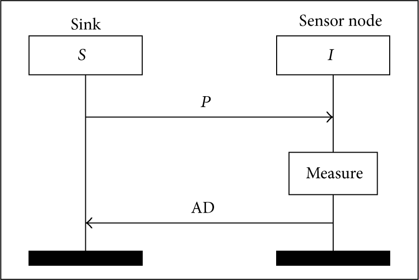
The flow of LOW security level protocol. The original protocol which ensures neither confidentiality nor authentication.

Figure 3

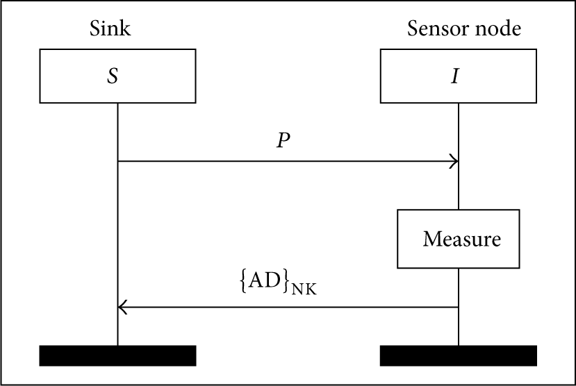
The flow of the MID security level protocol. The protocol encrypts the samples data with the AES-CTR-256 cipher and thus ensures confidentiality.

Figure 4

The flow of the HIGH security level protocol. Authentication is added by the use of the ECC with 160 bit key length.

In the LOW security level protocol, the Sink starts with message P containing the measurement parameters. Upon its reception, the Sensor starts measurement and sends back the acceleration data (AD), the result of the measurement. In this level no security attributes are guaranteed.

The MID security level protocol introduces confidentiality of accelerated data. After measurement, the Sensor encrypts the data with a predeployed network key (NK). In this protocol, the AES algorithm is chosen for the encryption in the CTR mode and with 256 bits of the key.

In the MID security level protocol, sensor nodes are not authenticated and a malicious node can deceive sensor nodes by impersonating the Sink and sending fake parameters P. This is avoided by the introduction of the sensors and parameters authentication achieved with the modified version of the DJS protocol from [28].

The HIGH security level protocol is started by sensor nodes. They generate key $K_{\text{DH}}(I,S)$ using the Diffie-Hellman method (ECC 160 bits of key) without communication with their private key and the Sink's public key as it is predeployed on all sensor nodes. The generated key is used to encrypt the request which is sent to the Sink. The request contains nonce $n_I$ and the Sensor's id (I). Upon receiving the request, the Sink decrypts it with the key generated using the same method as the sensors used and creates a response which contains the received nonce $n_I$ , a new nonce $n_{\text{AD}}$ , the Sink's id (S), the new session key used to encrypt data $K(I,S)$ , and parameters P. The response is encrypted with the Sensor's public key and sent back to the sensor. When the Sensor receives the parameters, it checks the nonce and starts the measurement process. When the process is finished, the acceleration data $\text{AD}$ and nonce $n_{\text{AD}}$ are encrypted with session key $K(I,S)$ and sent to the Sink. In this protocol, the AES algorithm is chosen for the encryption in the CTR mode and with 256 bits of the key.

Nonces $n_I$ and $n_{\text{AD}}$ are used to keep the messages fresh. Session key $K(I,S)$ which is generated by the Sink for each sensing session independently solves the problem of the distribution of the network key $\text{NK}$ appearing in the MID protocol.

The security mechanisms and metrics of cryptographic primitives for TelosB motes are described in [28]. The metrics for the electricity current are taken from [40].

The summary of the analysed cryptographic protocols which ensure security on different levels is presented in Table 3.

Table 3

Security levels evaluated in the case study.

Security level	Confidentiality	Authentication
LOW	—	—
MID	AES-CTR-256	—
HIGH	AES-CTR-256	ECC-160

6.2. Scenarios

The operation of the original version of the evaluated protocol consists of 4 sensing events per day. In this section, we introduce a situation in which the retrieved data needs to be more accurate. It takes place when the data retrieved from sensor nodes overcomes a threshold value. We defined ten scenarios in which the acceleration data is retrieved every hour for the subsequent 24 hours. Differences between scenarios are caused by various numbers of sensing events for each security level (LOW, MID, and HIGH) which are presented in Table 4. The introduction of the proposed scenarios largely increases the energy consumption of the network. Therefore, we want to evaluate several implementations with different levels of security and check their influence on energy consumption.

Table 4

The number of RemoteSensing events (sensing sessions) in a day for all scenarios.

	S.1	S.2	S.3	S.4	S.5	S.6	S.7	S.8	S.9	S.10
LOW level	4	0	0	24	0	0	4	20	20	8
MID level	0	4	0	0	24	0	0	0	4	8
HIGH level	0	0	4	0	0	24	20	4	0	8

The first three scenarios refer to the original version of the protocol where 4 sensing events are conducted. The difference comes from different security levels. The other scenarios refer to the situation with 24 sensing events.

As a result of the analysis, we predict the maximal energy consumption of the node and the lifetime of the network represented as the battery level remaining after given months of operation. In our case study, we assume that each node has two AA batteries with 1200 mAh capacity and take the maximal energy consumption of nodes as the energy consumption of the network for lifetime prediction.

7. Results

Table 5 contains the energy consumption and lifetime prediction results for the presented scenarios (Table 4).

Table 5

The energy consumption and lifetime prediction for all scenarios.

Scenario	Energy consumption (J)	Lifetime prediction (days)
S.1	43.34	299
S.2	68.99	187
S.3	75.20	172
S.4	260.06	49
S.5	413.92	31
S.6	451.21	28
S.7	378.90	34
S.8	262.01	49
S.9	261.90	49
S.10	294.16	44

The Energy consumption column contains the maximal amount of energy consumed by one sensor during the execution of one scenario.

The Lifetime prediction column contains the number of days passed before the battery of any sensor is depleted (according to the assumptions from Section 6.2).

The results from Table 5 show that various numbers of remote sensing events can have significant influence on the lifetime of wireless sensor networks. The lifetime of the first three scenarios is about 6 times longer because the number of sensing events is equally increased.

However, the lifetime of scenario number 4 (24 unsecured sensing events) is almost twice as long as the lifetime of the most secured scenario (number 6). The last scenario with the same number of sensing events for all three security levels seems to be a good compromise. The results show that the designers of WSN protocols should search for balance between the acceptable energy consumption and security level.

Obtained results suggest that in some situations ensuring security at the expense of energy consumption is inevitable. However, before implementing designed solutions, there is a need to carefully examine considered environment and choose the option which fulfills given requirements best (in terms of, for instance, time or energy consumption).

The proposed approach can automatically answer the question what is the difference in performance between the created scenarios. Through this analysis you can make a trade-off between the means of information protection and the required performance. In addition, this analysis allows us to create scenarios to cope with a situation that will require greater efficiency or security. Such events may include a sudden and significant change of environmental factors, for example, sudden weather change that implies stronger requirements for efficiency. On the other hand, the detection of unexpected communication can be treated as an attack and the stronger security is applied. To summarize, the system can switch the operation mode when such cases appear (adaptable security [15]).

8. Conclusions

In this paper, the authors present the advanced communication module as an extension of the QoP-ML. Described module allows us to perform complex network examination as part of protocol performance analysis. It is utilized to include the time and energy analysis of communication steps.

Another contribution of this paper is adding the energy analysis and lifetime prediction modules to the QoP-ML. The modification of the QoP-ML is also implemented as an extension to AQoPA tool, utilized for automatic use in performance analysis.

The authors use the proposed communication model to perform an analysis of an existing wireless sensor network deployed on the Jindo Bridge in South Korea. The aim of such an analysis is to predict the lifetime of the existing network with additional security attributes. The authors introduce new scenarios in which the operation of the actual sensor network is modified and the number of sensing events is increased in order to collect more precise acceleration data. In the case study, ten scenarios with miscellaneous security levels are analysed.

The results allow us to draw conclusions about the influence of security attributes on time and energy consumption of wireless sensor networks. In the presented case study it is shown that the introduction of security attributes can have significant influence on network lifetime. Therefore, the designers of WSN protocols should search for balance between the required lifetime and security level. The QoP-ML along with the AQoPA tool have been created to accomplish this task.