Data Collection for Time-Critical Applications in the Low-Duty-Cycle Wireless Sensor Networks

Abstract

In low-duty-cycle wireless sensor networks, wireless nodes usually have two states: active state and dormant state. The necessary condition for a successful wireless transmission is that both the sender and the receiver are awake. In this paper, we study the problem: How fast can raw data be collected from all source nodes to a sink in low-duty-cycle WSNs with general topology? Both the lower and upper tight bounds are given for this problem. We use TDMA scheduling on the same frequency channel and present centralized and distributed fast data collection algorithms to find an optimal solution in polynomial time when no interfering links happen. If interfering links happen, multichannel scheduling is introduced to eliminate them. We next propose a novel Receiver-based Channel and Time Scheduling (RCTS) algorithm to obtain the optimal solution. Based on real trace, extensive simulations are conducted and the results show that the proposed RCTS algorithm is significantly more efficient than the link schedule on one channel and achieves the lower bound. We also evaluate the proposed data collection algorithms and find that RCTS is time-efficient and suffices to eliminate most of the interference in both indoor and outdoor environment for moderate size networks.

1. Introduction

In most wireless sensor networks (WSNs), how to improve the network robustness for data collection is an important issue. Two seemingly contradictory, yet related objectives of performance exist: prolonging the network lifetime due to limited power resources and reducing data latency. On the one hand, researchers have put much effort to save or harvest energy for wireless sensor nodes in order to prolong the lifetime of individual nodes since most wireless sensor nodes are powered by batteries. On the other hand, some application scenarios like surveillance [1] require a bound on the data collection latency to guarantee availability of accurate information about the sensing field; otherwise, collected data information may become irrelevant or even useless [2, 3]. In many emergency applications, the collected sensor data are usually useful during a finite amount of time, after which the information may become irrelevant. The requirement is special in some time-critical application scenarios using WSNs, such as the application of monitoring the escapees’ current locations and expanding situation of hazard areas in the emergency navigation system [2]. In network diagnosis, it is necessary to collect metrics periodically, such as residual energy levels of nodes and instant network conditions, which are required to be collected in real time [3]. In the above situations, sensor data and metric information are both asked to be collected from nodes to the sink as soon as possible. Hence, the maximum end-to-end delay for each bit must be limited within some acceptable time-efficient requirement.

One of simple but efficient methods to prolong the lifetime of WSNs is to decrease the duty cycle of individual nodes [4–6] such that they finish coping with sensing and transmission operations when they are awake while falling into sleep for the rest of time in a time period. Hence, the working mode of sensor nodes is normally designed as periodic active in most monitoring applications [7, 8]. However, this brings forth another challenge for minimizing end-to-end delay since any individual node existing on some end-to-end transmission path makes the path unfeasible if it goes into dormant state such that the end-to-end delay cannot be controlled easily. In addition, the low-duty-cycle mechanism causes more severe collision because the available time for nodes to receive packets is notably reduced [6]. Several attempts have been applied to decrease the end-to-end latency for WSNs. For instance, [9] utilized collision-avoidance method to reduce interference among wireless transmission since the latter causes much retransmission due to packet loss, especially when a contention-based MAC protocol (e.g., CSMA) is explored. Some other work [10] also proved that one of the main reasons of traffic latency is the “wasting” sleeping time of the receiver.

In this paper, we focus on how to design Fast Data Collection algorithms to reach the minimum data collection delay in low-duty-cycle WSNs. We apply contention-free MAC protocols, that is, TDMA, to eliminate collisions and make the best of the limited link resources in compliance with node working schedules. In addition, since the network protocols can affect the end-to-end delay of each bit [10], we use a joint routing and scheduling cross-layer design to search the minimum data collection delay paths. To address fast data collection problem, we present both centralized and Distributed Fast Data Collection algorithms when no interfering links happen. If the interfering links happen, the multichannel scheduling is introduced to eliminate interfering links. Furthermore, a simple but efficient distributed channel and time scheduling method is proposed to search the minimum data collection delay paths. The main intellectual contributions of this work are summarized as follows.

• (1)

For the raw data collection, we define a minimum data collection delay (MDCD) problem and give both the upper and lower tight bounds on the data collection delay.

(2)

We present a novel Centralized Fast Data Collection (CFDC) algorithm (Algorithm 1), adopted to any general topology, which achieves the lower bound and returns the optimal collection paths with the minimum delay in polynomial time.

(3)

We further propose a Distributed Fast Data Collection (DFDC) algorithm based on the node's local information. It is proved that the DFDC algorithm can also obtain the optimal solution.

(4)

In order to eliminate the interfering links and guarantee network robustness, we present a Receiver-based Channel and Time Scheduling (RCTS) algorithm to the search for minimum data collection delay paths. The data trace based evaluations show the use of RCTS can suffice to eliminate most of the interference in both the indoor and outdoor environment.

Algorithm 1: Centralized Fast Data Collection algorithm.

Input: The given VGN over the time expanded.

Output: The optimal data collection paths with the minimum

delay.

(1) Initialization: $$\mathrm{\Delta }=\text{ma}{\text{x}}_{i=\mathrm{1}}^{n-\mathrm{1}}\{T_{\min }^i\}$$ , $$f_m=\mathrm{0}$$ , $$k=⌊\mathrm{\Delta }/T_{\pi }⌋$$

(2) while   $$f_m<n-\mathrm{1}$$   do

(3)  Update the sub-graph of VGN under the time threshold

    $$k{T}_{\pi }$$ .

(4)  while  there is an s-d path in the residual graph $$G_f(\mathrm{\Delta })$$

    do

(5)   P be a simple s-d path in $$G_f(\mathrm{\Delta })$$

(6)    $$f^{\prime }$$ = augment( $$f,P$$ )

(7)   if   $$f^{\prime }$$ satisfies the constraints in the above max-flow

    problem then

(8)     Update f to be $$f^{\prime }$$

(9)     Update the residual graph $$G_f(\mathrm{\Delta })$$ to be $$G_{f^{\prime }}(\mathrm{\Delta })$$

(10)  Obtain the maximum flow $$f_m$$ of $$(G,s,d,c,\mathrm{\Delta })$$ and

    optimal flow paths P.

(11)   $$k=k+\mathrm{1}$$

(12) Among the $$N_{i,t}$$ through flow in the kth $$T_{\pi }$$ period, find

  the the largest t of $$N_{i,t}$$ .

(13) $$T_{\min }$$ = the largest t.

The rest of this paper is organized as follows. Section 2 briefly presents the related work. We present the network model and formulate our problem formally in Section 3. In Section 4, both the upper and lower bounds are given on the MDCD problem. We propose a CFDC algorithm to solve the fast data collection problem when no interfering links happen, which obtains the optimal solution. In Section 5, a DFDC algorithm is further presented when no interfering links happen. When interfering links happen, combining with multiple channel scheduling, a RCTS algorithm is proposed to search for the minimum data collection delay paths in Section 6. Based on the data trace from the Berkeley Lab, extensive simulations are conducted in outdoor and indoor scenarios and further present and analyze the results in detail in Section 7. We conclude our paper and discuss future work in Section 8.

2. Related Work

The contribution of our work lies in the intersection of two important cutting-edge research topics: (1) the function performance of data collection and (2) the low-duty-cycle working modes of sensor nodes. We review some related work in both topics as follows.

Data Collection. The objective of most WSN-related applications is to collect data from physical world, such as environmental surveillance [8, 11] and vehicle and structural monitoring [12–15]. Some work [9, 16, 17] concentrated on how to improve the energy efficiency, time efficiency, and (or) reliability of deployed WSNs. In [16], the authors presented a practical, energy efficient, and reliable solution to the problem of periodic data collection. Reference [9] proposed a link scheduling algorithm finding the minimum delay schedule when the slot lengths of link are given. Basically, they investigated the tradeoff between the energy consumption and delay. By developing a novel and efficient TDMA schedule, [17] studied the effect of dynamic traffic patterns for data collection. However, for all the aforementioned work, the authors assumed that the data collection was applied in the case with constant availability of connectivity such that the proposed algorithms may lead to very low efficiency in low-duty-cycle sensor networks with sleep latency.

Low-Duty-Cycle. One of simple but efficient methods to prolong the lifetime of WSNs is to decrease the duty cycle of individual nodes such that they finish coping with sensing and transmission operations when they are awake while falling into sleep for the rest of time in a time period since a node almost costs no energy in dormant state. Some other work studied the low-duty-cycle related topics from different points of view, such as data flooding and broadcasting [10, 18], sleep scheduling [5, 19], and multiple tasks scheduling [6]. In [10], the authors detailed an opportunistic flooding method in a low-duty-cycle WSN with unreliable links when the working schedules of all wireless sensor nodes were given. Reference [18] aimed to solve the latency-optimal broadcasting problem in the duty-cycled multihop wireless networks and proposed three algorithms to improve the approximation ratios. They also proposed a forwarder selection method to alleviate the hidden terminal problem. The work [19] modified the random duty cycling to solve slow diffusion problem. Reference [5] introduced energy-efficient sleep scheduling in order to minimize latency. The authors of [6] provided two efficient scheduling algorithms in order to balance network traffic. However, most of above work regarding low-duty-cycle WSNs does not concern data collection function.

Some work, like [4, 20], has similar objectives with our problem. In [4], the authors presented a dynamic data forwarding $(\mathrm{D}\mathrm{S}\mathrm{F})$ scheme in extremely low-duty-cycle sensor networks with unreliable links. They studied the impact of both lossy radio link and sleep latency at the network layer. Although the $\mathrm{D}\mathrm{S}\mathrm{F}$ scheme can be used to data collection scenario in low-duty-cycle networks, it adopted some multiple paths routing strategy which suffered packet duplicated issue inevitably. In addition, exchanging traffic statistic frequently for routing cutover may introduce nonnegligible communication overhead. Reference [20] provided cross-layer analysis framework for end-to-end delay distribution in WSNs. Some MAC protocols, such as B-MAC [21], exploited network information like packet transmission or routing paths to optimize their link scheduling. Reference [4] considered the MAC layer information (like link quality) into the network layer, which leads to better link selections.

For the interference elimination, the use of multiple channels has been studied extensively in both cellular and ad hoc networks. However, in the domain of wireless sensor networks, there exist some research that utilize multiple channels [22].

To the best of our knowledge, there is no prior work that has thoroughly researched on the optimal delay routing algorithm for the data collection scenario in low-duty-cycle sensor networks without topology constraints. In this work, by taking the available time of link resources (working schedules) into consideration, we reveal that the cross-layer design is to obtain a delay-optimal data collection path for each wireless sensor node and exploit multiple-channel scheduling to eliminate the interfering links.

3. Network Model and Problem Formulation

In this section, we first focus on a TDMA scheduling cross-layer design when the nodes communicate on the same channel without any interfering link present. In the following Section 6, the case where interfering links happen is considered. We will combine with the multichannel scheduling to eliminate the interfering links without compromising the time efficiency of data collection.

3.1. Network Model

In this work, it is considered that a connected network with n wireless sensor nodes works in a low-duty-cycle mode. Basically, each sensor node has two states: active and dormant. When a node is in active state, it can sense or receive packets from neighbor nodes. For the purpose of energy conservation, a node in dormant turns off all its functional models except a timer to wake itself up. Under the low-duty-cycle working mode, if a node only delivers packets in active state, the packets will hardly be sent out since the active time may not overlap with that of its neighbors. To solve this problem, each node still receive packets when it is in active state, but the transmission rule is changed as follows: if a node has packets to forward beyond its active time slots, it wakes up its transceiver and transmits packets when its next hop neighbor turns into active state [23].

To simplify the discussion, it is assumed that all nodes in the network work in the asynchronous duty-cycle mode and are sources except the sink. The objective is to minimize the whole time T required to complete data collection. In TDMA MAC protocol, T is divided into a number of equal-length time slots τ, each of which is long enough to transmit one packet successfully. We also assume that each node wakes up to receive the packet for only one time slot in every cycle, which is reasonable since the function of low-duty-cycle aims to reduce the waking time of individual node [24].

To symbolize the working schedule more clearly, we describe it as a binary string for individual node, in which $\mathrm{1}$ means the node in active state, while $\mathrm{0}$ indicates that in dormant state [4]. The cycle period of working schedule is denoted as $T_{\pi }$ . For example, the working schedule of node $n_i$ can be extended to ${\pi }_i^T=\mathrm{0100010001}$ , if the network collecting time T is 10 time slots, ${\pi }_i=\mathrm{0100}$ and $T_{\pi }$ is 4 time slots. The above assumption is the same as the previous work [4, 10, 23].

There are two common types of interference models: the graph based protocol model and the SINR-based physical model. In the protocol model, the transmission from node i to a node j is successful, if for every other k, simultaneously transmitting, the following condition holds:

$$\begin{array}{cc}& d\left(k,j\right)\ge \left(\mathrm{1}+\Delta \right)d\left(i,j\right),\hspace{1em}\left(\Delta >\mathrm{0}\right),\end{array}$$

(1)

where $d(i,j)$ is the distance between node i and node j and δ is a parameter that promise that the concurrently transmitting nodes are enough far away from the receiver to prevent interference.

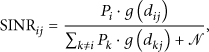
The physical model considers the accumulative effect from multiple concurrent transmissions. The transmission of a packet from node i to node j is successful when the ratio between the received signal strength at node j and the cumulative interference caused by all other concurrent transmissions and the background noise is greater than a certain threshold β; that is,

$$\begin{array}{cc}& {\mathrm{S}\mathrm{I}\mathrm{N}\mathrm{R}}_{ij}=\frac{P_i·g\left(d_{ij}\right)}{{\sum }_{k\ne i}‍P_k·g\left(d_{kj}\right)+\mathcal{N}},\end{array}$$

(2)

where $P_i$ is the transmission power at node i, ${\mathrm{S}\mathrm{I}\mathrm{N}\mathrm{R}}_{ij}$ indicates the signal-to-interference-plus-noise ratio, $\mathcal{N}$ is the background noise level, $g(·)$ is the signal attenuation function, and $d_{ij}$ is the distance between nodes i and j. Since all nodes use the same constant transmission power, we set $P_i=P_k=\mathrm{1}$ . For simplicity of exposition, we use a simple distance dependent path-loss model as $g_{ij}=d_{ij}^{-{\alpha }_{ij}}$ , where the path-loss exponent ${\alpha }_{ij}$ is a factor between $\mathrm{2}$ and $\mathrm{6}$ , depending on the external wireless environment, such as humidity, temperature, and obstacles. It is assumed that the interference level in both models is static and does not change over time.

Reference [25] found that the use of the graph based model fails most in sparse network deployments with higher path-loss exponents, and the physical interference model is closer to the actual situation than the protocol model. Hence, we use the physical model in all the following evaluation cases.

3.2. Problem Formulation

We define the MDCD problem as follows. Given a WSN with n sensor nodes, if the sink node is the nth node, the other $n-\mathrm{1}$ nodes are source nodes, each of which generates one packet. Collection delay is defined as the time elapsed from packets being generated until all $n-\mathrm{1}$ packets reach the sink. The goal is to find data collection paths to the sink from each source with the minimum collection delay. Symbol $\mathrm{E}\mathrm{E}\mathrm{D}(v_i)$ is used to denote the end-to-end delay (EED) for source node $v_i$ to the sink within either one or multiple hops. The objective is to minimize $T={\mathrm{m}\mathrm{a}\mathrm{x}}_{i=\mathrm{1}}^{n-\mathrm{1}}\mathrm{E}\mathrm{E}\mathrm{D}(v_i)$ , $\forall v_i\in V$ .

Formally, let $x(i,j,t)$ be a $\mathrm{1}-\mathrm{0}$ integer variable indicating whether the node $v_j$ at time t receives data from $v_i$ . $H_j$ indicates the active time of node $v_j$ and $c(p_i,j,t)$ is also a Boolean variable denoting whether the packet $p_i$ is delivered by node $v_j$ at time t. Thus, the MDCD problem can be described as follows.

•  

Problem: Minimizing Data Collection Delay

 

Objective: Minimize T

 

Subject to:

$$\begin{array}{r}{\displaystyle \sum }_{i=\mathrm{1},i\ne j}^{n-\mathrm{1}}‍x\left(i,j,t_{\mathrm{1}}\right)+{\displaystyle \sum }_{m=\mathrm{1},m\ne j}^{n-\mathrm{1}}‍x\left(j,m,t_{\mathrm{2}}\right)\le \mathrm{1},\\ \mathrm{w}\mathrm{h}\mathrm{e}\mathrm{r}\mathrm{e}\mathrm{\hspace{0.17em}\hspace{0.17em}}{t}_{\mathrm{1}}\in H_j,\hspace{0.17em}{t}_{\mathrm{2}}\in H_m\end{array}$$

(3)

$$\begin{array}{c}{\displaystyle \sum }_{t=\mathrm{1}}^T‍c\left(p_i,j,t\right)\le \mathrm{1},\hspace{1em}\mathrm{w}\mathrm{h}\mathrm{e}\mathrm{r}\mathrm{e}\hspace{0.17em}\hspace{0.17em}t\in \left[\mathrm{0},T\right]\end{array}$$

(4)

$$\begin{array}{c}x\left(i,j,t_{\mathrm{3}}\right)=\mathrm{0},\hspace{1em}\mathrm{w}\mathrm{h}\mathrm{e}\mathrm{r}\mathrm{e}\hspace{0.17em}\hspace{0.17em}{t}_{\mathrm{3}}\in \left[\mathrm{0},T\right],\hspace{0.17em}{t}_{\mathrm{3}}\notin H_j.\end{array}$$

(5)

Here, inequality (3) ensures that each node in active time can only receive one packet from its neighbor node and cannot receive or send data simultaneously. The links in Figure 1(a) can not be scheduled simultaneously. Inequality (4) guarantees that the same packet can only be delivered once by each node, which can restrict routing loops in the network. Equation (5) restricts the ability of each node to receive data when it is in dormant state.

Figure 1

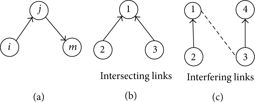
The constraints for links scheduling.

In terms of collision type, the links for interference are divided into two categories: intersecting links and interfering links [25]. The intersecting links, defined as the links with a common destination shown in Figure 1(b), cannot transmit on the same time slot since there is only one half-duplex radio transmitter in a sensor node. The constraint described by inequality (3) ensures that the intersecting links will not exist in the data collection paths. The interfering links are the links which create or face interference if they are scheduled simultaneously, which happens when two nodes send data simultaneously, and the SINR of any receiver is not greater than the predefined threshold. Figure 1(c) shows an example where the dotted line represents interference. Interfering links should not get the same time slot and channel. Since our goal is to minimize the number of time slots, the best option is to assign the same time slot on nonconflicting channels. Hence, the interfering links can be avoided to exploit the orthogonal frequencies [24, 25], that is, using multiple frequency channels to enable more concurrent transmissions. In the following study cases, we first consider MDCD problem in a case where nodes communicate on the same channel with the goal of minimizing the data collection delay. Next, we combine with the multichannel scheduling to avoid the interfering links.

4. Centralized Fast Data Collection Algorithm

In this section the goal is to address the MDCD problem. We first analyze the lower and upper bounds on the delay for data collection and give the procedure of proofs. Furthermore, we introduce a novel concept, the VGN to convert the MDCD problem into max-flow problem with special constraints. Based on VGN, we propose a Centralized Fast Data Collection algorithm (CFDC) to obtain the optimal collection paths with minimum delay in polynomial time when no interfering links happen.

4.1. The Lower and Upper Bounds on the Data Collection Delay

Lemma 1.

The delay for data collection is tightly lower bounded by $S(sink)+(N-\mathrm{1})T_{\pi }$ , where $T_{\pi }$ denotes cycle period of working schedule, $S(sink)$ is the active start time of the sink in $T_{\pi }$ , and N is the number of source nodes.

Proof.

The detailed proof can be seen in our previous work [26].

Lemma 2.

The delay for data collection is tightly upper bounded by ${\sum }_{i=\mathrm{1}}^N{T}_{\mathrm{m}\mathrm{i}\mathrm{n}}^i$ , where N is the number of source nodes and $T_{\mathrm{m}\mathrm{i}\mathrm{n}}^i$ denotes the minimum time that source node i requires to deliver a packet to the sink without the effect of other packets.

Proof.

The detailed proof can also be seen in our previous work [26].

4.2. Virtual Grid Network

To make the node states and packet transmission process more clear, we define and detail a concept, VGN inspired by the time-expanded network proposed in [4]. The edge construction regulations of VGN are different from the time-expanded network. We first show how to construct the VGN based on the original directed communication graph G, which is the foundation of the data collection method proposed later.

For simple presentation, we first classify the nodes in G into three types by different roles.

• (i)

Leaf node: only acts as a source node; that is, it transmits its own sensor reading.

(ii)

Intermediate node: acts as double roles of a source node and a relay node; that is, not only does it transmit its sensor reading, but also receives a packet and tries to forward it when its neighbors awake. The own generated packet has higher priority to transmit than the forwarded packets.

(iii)

Sink node: responsible for receiving packets.

A deployed WSN is transferred into a communication graph $G=(V,E)$ , where V denotes the node set with cardinality n and E is the edge set. Assume that the working schedule for each wireless node $n_i\in V$ is given; we build a VGN according to the following rules.

• (1)

For each node $n_i$ active at time $t\in [\mathrm{0},T]$ , we build a virtual active node $N_{i,t}$ in VGN.

(2)

When node $n_i$ is a leaf node and has a directed edge to the node $n_j$ in G, if the first active time of $n_i$ is t and the active time of node $n_j$ is p after time t, we add a directed edge from $N_{i,t}$ to $N_{j,p}$ in VGN. Since the leaf node only transmits its own sensor reading, it is not possible for $n_i$ to have new arrived packet at the other active time except the first one.

(3)

When node $n_i$ is an intermediate node and has a directed edge to the node $n_j$ in G, if the active time of node $n_i$ and $n_j$ are t and p ( $p,t\in [\mathrm{0},T]$ ), respectively, and $p>t$ , we add a directed edge from $N_{i,t}$ to $N_{j,p}$ in VGN.

For the raw data collection, the MDCD problem can obtain an optimal result by reducing into the max-flow problem. In order to formulate a max-flow problem over the VGN, we introduce two virtual vertices, the super source and the super sink, symbolized by s and d, respectively, to represent the source and destination of the total flow over the graph. We complement the rules to build the connection from s and d to the virtual active nodes.

• (4)

When node $n_i$ is a sink, we connect all its corresponding virtual active nodes to the super sink d.

(5)

We build the edges from the super source s to the corresponding first active virtual nodes of all source nodes.

Here, the first rule illustrates the regulations to establish all nodes of VGN. The remainder rules depict how to build edges to connect nodes in VGN according to G. We take the simple network in the best case mentioned in Figure 2 as an example to give a walk-through of VGN construction (shown in Figure 4).

Figure 2

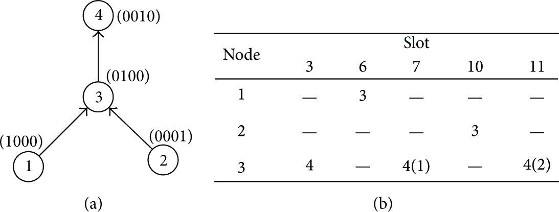
One of the best cases. (a) A network topology with given working schedule of each node. (b) Node ids from which packets are received by their corresponding parents in different time slots.

In the following, we detail how to construct VGN graph in terms of original network topology and working schedule of each node. First, we set the nodes in VGN based on the working schedule of each node in G by Rule $\mathrm{1}$ and the red nodes in VGN represent the virtual active nodes. Next, we describe how to construct corresponding edges in VGN according to Rules 2–5.

For the leaf node $v_{\mathrm{1}}$ , it can send a packet to its neighbor $v_{\mathrm{3}}$ when $v_{\mathrm{3}}$ is active. Thus, we establish the edges of $N_{\mathrm{1,1}}\to N_{\mathrm{3,2}}$ , $N_{\mathrm{1,1}}\to N_{\mathrm{3,6}}$ , and $N_{\mathrm{1,1}}\to N_{\mathrm{3,10}}$ in VGN by Rule $\mathrm{2}$ . For another leaf node $v_{\mathrm{2}}$ , it can also send a packet to its neighbor $v_{\mathrm{3}}$ when $v_{\mathrm{3}}$ is active. According to the same rule, we build the edges of $N_{\mathrm{2,4}}\to N_{\mathrm{3,6}}$ and $N_{\mathrm{2,4}}\to N_{\mathrm{3,10}}$ in VGN.

For the intermediate node $v_{\mathrm{3}}$ , it can send a packet to its neighbor $v_{\mathrm{4}}$ when $v_{\mathrm{4}}$ is active. Hence, we establish the edges from $N_{\mathrm{3,2}}\to N_{\mathrm{4,3}}$ , $N_{\mathrm{3,2}}\to N_{\mathrm{4,7}}$ , and $N_{\mathrm{3,2}}\to N_{\mathrm{4,11}}$ in VGN. At the same time, as a relay node, node $v_{\mathrm{3}}$ can receive packets when it turns to be active and forwards packets when its neighbor is active. Accordingly, we establish the edges $N_{\mathrm{3,6}}\to N_{\mathrm{4,7}}$ , $N_{\mathrm{3,6}}\to N_{\mathrm{4,11}}$ , and $N_{\mathrm{3,10}}\to N_{\mathrm{4,11}}$ in VGN.

For the sink $v_{\mathrm{4}}$ , we build the edges from the corresponding virtual active nodes to the super sink d by Rule $\mathrm{4}$ , that is, $N_{\mathrm{4,3}}\to d$ , $N_{\mathrm{4,7}}\to d$ , and $N_{\mathrm{4,11}}\to d$ . Finally, we build the connection from the super source s to the corresponding first active virtual nodes of all source nodes by Rule $\mathrm{5}$ , that is, $s\to N_{\mathrm{1,1}}$ , $s\to N_{\mathrm{2,4}}$ , and $s\to N_{\mathrm{3,2}}$ . The whole mapping process for one of the best cases is completed, as shown in Figure 4.

4.3. The Max-Flow Problem with Transmission Constraints

Given the VGN, our next step is the formulation of an optimization problem whose objective is to maximize the flow from s to d, that is, the most number of source nodes from which the sink can collect data successfully under the given time duration T. $f(\ast ,\ast )$ indicates the binary traffic flow over an edge connecting two vertices in VGN. Denoting by $F(\ast ,\ast )$ the total flow from the source to the destination, our objective can be described as

$$\begin{array}{cc}& \mathrm{m}\mathrm{a}\mathrm{x}\left\{F\left(s,d\right)\right\}.\end{array}$$

(6)

The data collection delay is defined as the total time required to complete data collection, which depends on the maximum EED for each source node. Minimizing the maximum EED problem is equal to the max-flow problem in VGN, which needs to be solved taking into account several constraints due to, for example, interference influence and half-duplex transceiver limitation. We detail such constraints below.

Constraints

Nonnegative Flow and Flow Conservation. The flow on every existing edge must be greater than or equal to zero. In the meantime, for any vertex in the VGN, the amount of flow entering the vertex must be equal to the amount of outgoing flow. Mapping to the VGN, the constraint can be expressed as

$$\begin{array}{r}{\displaystyle \sum }_{p\in N\left(i\right)}‍f\left(N_{p,t_p},N_{i,t}\right)={\displaystyle \sum }_{q\in N\left(i\right)}‍f\left(N_{i,t},N_{q,t_q}\right),\\ \mathrm{w}\mathrm{h}\mathrm{e}\mathrm{r}\mathrm{e}\mathrm{\hspace{0.17em}\hspace{0.17em}}{t}_p<t<t_q\in \left[\mathrm{0},T\right].\end{array}$$

(7)

The function $N(i)$ indicates the set of node i's neighbors in the original network G.

Half-Duplex Transceiver Limitation. Due to the hardware function limitation, a node cannot transmit and receive packets simultaneously shown in Figure 1(a). Mapping to the VGN, the constraint can be expressed as

$$\begin{array}{r}f\left(N_{i,t_{\mathrm{1}}},N_{j,t_{\mathrm{2}}}\right)+f\left(N_{j,t_{\mathrm{3}}},N_{m,t_{\mathrm{2}}}\right)\le \mathrm{1}\\ \mathrm{w}\mathrm{h}\mathrm{e}\mathrm{r}\mathrm{e}\hspace{0.17em}\hspace{0.17em}{t}_{\mathrm{1}},t_{\mathrm{2}},t_{\mathrm{3}}\in \left[\mathrm{0},T\right],\end{array}$$

(8)

where the binary function f( $\ast ,\ast$ ) is equal to $\mathrm{1}$ if the edge carries a flow; otherwise it is $\mathrm{0}$ . We notice that the case shown in Figure 1(a) happens only when j and m are the neighbors and active at the same time in the original topology.

Meanwhile, a node cannot receive from more than one neighbor at the same time, shown in Figure 1(b). For this constraint, we set the node capacity in VGN to one unit, that is, $C_{N_{i,t}}=\mathrm{1}$ . We can deduce that the edge capacity in VGN satisfies the conditions below:

$$\begin{array}{cc}& {\displaystyle \sum }_{p\in N\left(i\right)}‍f\left(N_{p,t_p},N_{i,t}\right)\le C_{N_{i,t}}=\mathrm{1},\hspace{1em}\mathrm{w}\mathrm{h}\mathrm{e}\mathrm{r}\mathrm{e}\hspace{0.17em}\hspace{0.17em}{t}_p\le t\in \left[\mathrm{0},T\right],\\ {\displaystyle \sum }_{q\in N\left(i\right)}‍f\left(N_{i,t},N_{q,t_q}\right)\le C_{N_{i,t}}=\mathrm{1},\hspace{1em}\mathrm{w}\mathrm{h}\mathrm{e}\mathrm{r}\mathrm{e}\hspace{0.17em}\hspace{0.17em}t\le t_q\in \left[\mathrm{0},T\right].\end{array}$$

(9)

Since we assume that the interfering links are eliminated, the max-flow problem is completed to formulate.

4.4. Minimum Data Collection Delay Algorithm

After converting the MDCD problem into a max-flow problem, we present a novel CFDC algorithm inspired by the Ford-Fulkerson max-flow method to solve the MDCD problem and obtain the optimal solution in polynomial time.

In CFDC algorithm, the working schedule for each node needs to be known by the sink in the network initialization, which can be easily achieved through exchange of the hello messages. The initial expanding time of VGN is set to be the maximum value of the set of minimum time for each packet delivered to the sink by Dijkstra Algorithm. The maximum flow $f_m$ is set to zero at the initialization step. Each iteration of the outmost while-loop corresponds to one phase. In each phase, the time threshold T is monotonously increased with the step of cycle period $T_{\pi }$ . The number of phases stops to increase until the maximum flow satisfied by all constraints is equal to the number of source nodes. This is an indication that all packets can be scheduled within T without collision. Obviously, the result P is the optimal collection paths for all source nodes.

Theorem 3.

If all the interfering links are eliminated, CFDC algorithm can obtain the optimal data collection paths with the minimum delay, that is, $S(sink)+(N-\mathrm{1})T_{\pi }$ .

Proof.

The max-flow problem is to find the max flow from the source s to the destination d. In the VGN, the neighbors of super sink come from the corresponding virtual active nodes of the sink. Therefore, in order to make the flow maximum from s to d, the corresponding virtual active nodes of the sink try to carry flow as much as possible. When all corresponding virtual active nodes of the sink carry flow, the sink keeps receiving packets in all active time. At this moment, CFDC algorithm returns the optimal collection path with the minimum delay, that is, $S(\mathrm{s}\mathrm{i}\mathrm{n}\mathrm{k})+(N-\mathrm{1})T_{\pi }$ . In the best case illustrated above, the optimal collection paths returned by CFDC algorithm are shown in bold in Figure 4, and the minimum collection delay achieves the lower bound. Thus, the CFDC algorithm can obtain the optimal collection paths with the minimum delay.

In addition, due to the half-duplex transceiver constraints, it sometimes fails to make all corresponding virtual active nodes of the sink carried flow, shown in the worst case mentioned above (Figure 3). But it can also obtain the optimal solution. Figure 5 shows the optimal collection paths returned by CFDC algorithm. However, the returned minimum delay will not achieve the lower bound, since it applies in the best case.

Figure 3

One of the worst cases. (a) A network topology with given working schedule of each node. (b) Node ids from which packets are received by their corresponding parents in different time slots.

Figure 4

VGN transformation. (a) A simple network. (b) The Virtual Grid Network.

Figure 5

The optimal data collection paths of the worst case returned by the CFDC algorithm.

Lemma 4.

The total time complexity for CFDC algorithm is $O(T^{\mathrm{3}}{n}^{\mathrm{3}})$ . Here, T is the minimum time threshold when the maximum flow is equal to the number of source nodes.

Proof.

The detailed proof can be seen in [26].

5. Distributed Fast Data Collection Algorithm

Since the CFDC needs to obtain all nodes cycling information, it is not practical to implement the CFDC in the large scale networks. In this section, we present the distributed version of our Fast Data Collection algorithm. We first analyze the generic principle for link scheduling and then we propose a Distributed Fast Data Collection (DFDC) algorithm to reduce the beacon overhead. Finally, we present the theoretical analysis of DFDC.

5.1. Design Philosophy

Such CFDC is a link-based method and is difficult to be performed in a distributed environment. This is because it needs the information of all potential links to construct VGN, which brings out large overheads. We aim to design a node-based method to solve MDCD problem, by which the node make a decision by itself. That means the node decides locally what its next hop is, and when the data is delivered.

The main idea are as follows: (1) Keep the sink busy in receiving packets for as many active time slots as possible. Because the sink has duty cycle, we need to guarantee the nodes within one hop to the sink always waiting for sending packets. (2) Give higher priority to the node to send data that is nearer to the sink. The number of hops from node to the sink is represented as the distance to the sink by Dijkstra shortest path algorithm.

Definition 5.

The pressure index of node $i\in n$ , denoted by $p(i)$ , is the minimum number of hops from node i to the sink by Dijkstra shortest path algorithm, which represents the distance to the sink.

Since the nodes far away from the sink are more difficult to send packets to the sink, they have higher pressure to deliver their packets.

5.2. Algorithm Description

The formal description of DFDC is shown in Algorithm 2.

Algorithm 2: Distributed Fast Data Collection algorithm.

Input: The original network topology

Output: The optimal link schedule solution with the minimum

delay.

(1) source-node.buffer = full

(2) Compute $$p(i)$$ for each node $$i\in n$$

(3) Sort nodes in the ascending order of $$p(i)$$

(4) while Any node's buffer is full do

(5)  for Each node i in the sorted order of V  do

(6)   if node.buffer == $$full$$   then

(7)    for Each node ∈i's neighbors who are active do

(8)     if  p(i.neighbor) $$<p\left(i\right)$$ and i.neighbor.buffer ==

       $$empty$$   then

(9)      i.neighbor is node i's next hop

(10)      i.neighbor.buffer = $$full$$

(11)      i.buffer = $$empty$$

Each source node keeps a buffer and its corresponding state, which is logical, either full or empty. The proposed DFDC algorithm does not require large buffers, because it is guaranteed that at any time the buffer will store not more than one packet. We initialize that all source nodes’ buffers are full and keep the sink's buffer always empty for ease of explanation.

We first sort all nodes based on the pressure index. For each time slot, packets then go through each node $i\in V$ in the sorted order and are pushed from nodes with higher $p(i)$ to ones with lower $p(i)$ step by step, until all packets are delivered to the sink. When node i decides its next hop, it will communicate with its neighbors and find the ones that satisfy two constraints: (1) the neighbors’ $p(i)$ is lower than the current node's; (2) the neighbors’ buffers are empty. For the result of finding conditional neighbors, there are three cases: (1) There is only one neighbor meeting both of constraints and then this neighbor is selected as the next hop. (2) There is more than one neighbor satisfying the above two conditions and then we choose one of them at random as the next hop. (3) There are no conditional neighbors; then the node will wait for another time slot until it has conditional neighbors to send its packet.

5.3. A Walk-Through Example

In Figures 6(a) and 6(b), we show the results of link scheduling in one of the best cases and one of the worst cases. Both of the original networks shown in Figure 6 contain four source nodes. The solid lines represent potential links when the receivers are active. The numbers beside the links represent the time slots at which the links are scheduled to send packets, and the numbers inside the circles denote nodes’ IDs.

Figure 6

Link schedule using DFDC algorithm: (a) One of the best cases. (b) One of the worst cases.

We run through an example shown in Figure 6(a) to explain the DFDC algorithm. We first compute the pressure index of each node and obtain that $p(\mathrm{1})=p(\mathrm{2})=\mathrm{2}$ , $p(\mathrm{3})=p(\mathrm{4})=\mathrm{1}$ , and $p(\mathrm{5})=\mathrm{0}$ . In the first duty cycle, since only the sink (node 5)'s buffer is empty and $p(\mathrm{5})$ is smaller than $p(\mathrm{4})$ , we schedule the link (4,5) when node $\mathrm{5}$ is active. Thus, the sink receives a packet from node $\mathrm{4}$ in slot $\mathrm{3}$ . In the second duty cycle, the buffers of node $\mathrm{3}$ and node $\mathrm{5}$ are empty and $p(\mathrm{3})<p(\mathrm{1})$ , $p(\mathrm{5})<p(\mathrm{4})$ ; thus we schedule the links (1,3) and (4,5) in slots $\mathrm{6}$ and $\mathrm{7}$ , respectively. Then the buffers of nodes $\mathrm{1}$ and $\mathrm{4}$ are empty. In the third duty cycle, the node $\mathrm{2}$ 's buffer is full and one of its neighbors, node $\mathrm{4}$ 's buffer, is empty. Thus we schedule the link (2,4) in slot $\mathrm{9}$ . For the same reason, we schedule the link (3,5) in slot $\mathrm{11}$ . Hence, the buffers of nodes $\mathrm{2}$ and $\mathrm{3}$ are empty. In the fourth duty cycle, only node $\mathrm{4}$ 's buffer is full. Hence we schedule the link ( $\mathrm{4,5}$ ) in slot $\mathrm{15}$ . This process continues until all the packets are delivered to the sink, yielding a link schedule that requires $\mathrm{15}$ time slots. In Figure 6(b), we show an assignment in one of the worst cases when all the interfering links are eliminated, yielding a schedule length of $\mathrm{27}$ time slots.

5.4. Algorithm Analysis

In the following, we prove that the DFDC algorithm can obtain the optimal solution when no interfering links happen. Before giving the detailed proof, we first highlight the two main principles of the algorithm: (1) The sink is kept in receiving packets for as many time slots as possible. (2) A node's buffer is not empty for two or more consecutive duty cycles as long as the buffers of one or more nodes with higher $p(i)$ are full. The first one is easy to prove by the scheduling rules of DFDC algorithm. We prove the second one in the following lemma.

Lemma 6.

At least one node with $p(i)=\mathrm{1}$ has full buffer during two consecutive duty cycles if one or more nodes with $p(i)>\mathrm{1}$ have full buffers.

Proof.

We prove it by induction on time slot $t=k{T}_{\pi }+\mathrm{1}$ . We focus on the first slot of each duty cycle. At $t=\mathrm{1}$ , the theorem is intuitively true because all buffers of the source nodes are full. Suppose the lemma holds for $t=k{T}_{\pi }+\mathrm{1}$ ; that is, for slot $t=k{T}_{\pi }+\mathrm{1}$ the buffers of all nodes with $p(i)=\mathrm{1}$ are empty, and for slots $t=(k-\mathrm{1})T_{\pi }+\mathrm{1}$ and $t=(k+\mathrm{1})T_{\pi }+\mathrm{1}$ there exists at least one node with $p(i)=\mathrm{1}$ whose buffer is full. At $t=(k+\mathrm{1})T_{\pi }+\mathrm{1}$ , one node $p(i)=\mathrm{1}$ whose buffer is full sends a packet to the sink, and its buffer becomes empty. There exist the following two cases: (1) all nodes with $p(i)=\mathrm{1}$ whose buffers are empty and at least one node with $p(i)=\mathrm{1}$ whose buffer is full at the following slot $t=(k+\mathrm{2})T_{\pi }+\mathrm{1}$ . (2) another node with $p(i)=\mathrm{1}$ whose buffer is full, which is noted as node j.

The first case means that, for slot $t=k{T}_{\pi }+\mathrm{1}$ , there is only one node with $p(i)=\mathrm{1}$ , whose buffer is full. Since there is one or more nodes with $p(i)>\mathrm{1}$ in full buffers, during the next duty cycle, the nodes with $p(i)=\mathrm{1}$ will receive at least one packet.

The second case means that, for slot $t=k{T}_{\pi }+\mathrm{1}$ , there are more than one node with $p(i)=\mathrm{1}$ , whose buffers are full. For slot $t=(k+\mathrm{1})T_{\pi }+\mathrm{1}$ , one node with $p(i)=\mathrm{1}$ whose buffer is full sends a packet to the sink. Since the sink only receives one packet during each duty cycle, there is another node with $p(i)=\mathrm{1}$ , whose buffer is full. Therefore, the lemma holds for $t=(k+\mathrm{1})T_{\pi }+\mathrm{1}$ , and the proof follows.

Theorem 7.

DFDC algorithm can obtain the optimal data collection paths with the minimum delay, that is, $S(sink)+(N-\mathrm{1})T_{\pi }$ .

Proof.

The principle of DFDC algorithm is to keep the nodes with $p(i)=\mathrm{1}$ always waiting for sending a packet. From Lemma 6, we know that the sink keeps receiving a packet during two consecutive duty cycles. Therefore, the DFDC algorithm can obtain the optimal data collection paths with the minimum delay. Note that the lower bound of the best case illustrated in Figure 6 is $S(\mathrm{s}\mathrm{i}\mathrm{n}\mathrm{k})+(N-\mathrm{1})T_{\pi }=\mathrm{3}+\mathrm{3}\times \mathrm{4}=\mathrm{15}$ , the same as the result of the proposed DFCD algorithm.

6. Impact of Interference

So far, we consider the scheduling methods which assign the same channel to all the receivers. Since all communications on the same channel can not avoid the interfering links, the collision will happen if the SINR value at any receiver is not greater than the predefined threshold, especially when two or more transmissions are launched at the same time slot. In this section, we combine the channel with time scheduling to eliminate the interfering links.

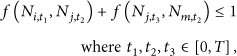
As shown in Figure 6(b), links $(\mathrm{4,5})$ and $(\mathrm{1,3})$ at slot $\mathrm{11}$ as well as links $(\mathrm{4,5})$ and $(\mathrm{2,3})$ at slot $\mathrm{19}$ are interfering links. If the interfering links are scheduled at the same channel, it will result in serious data loss. We give the experimental results to show how serious it is when the density is on the rise. In the 100 m square field, varied number of nodes are deployed randomly and we evaluate the delivery ratio along with the increase of node density. From Figure 7, we observe that the delivery ratio deteriorates when all communications are scheduled on the same channel, especially in high network density. The main reason is that interfering links cause massive collisions. The easy way to avoid the interfering links is to assign extra time slots, however it results in the large delay of data collection. If all the interfering links are present, the total schedule length will extend to 35 slots for the case in Figure 6(b). Without compromising the time efficiency of data collection, we use multiple frequency channels to avoid the interfering links.

Figure 7

Delivery Ratio under different duty cycle.

We propose a simple Receiver-based Channel and Time Scheduling (RCTS) algorithm which assigns the time slots and channels based on DFDC algorithm. Since the data transmission depends on the time slot when the receiver wakes up, we first use DFDC algorithm to assign links on the same channel. Next, for receivers working at the same slot, it is checked whether any interfered receiver based on SINR thresholds exists and assigns the next available channel iteratively starting from the interfered receiver with the lowest $p(i)$ . Note that we assume there are adequate channels available to be allocated to the interfered receivers.

7. Performance Evaluation

In this section, we evaluate the impact of duty cycle, multiple channels for both the outdoor and indoor environment under the physical interference model.

Simulation Setup. A sink is positioned in the center of deployment field, and each sensor node sends its packet to the sink over single or multiple hops. The working schedules of all the nodes are predefined by picking their one active slot randomly in a cycle period, which will be fixed through the data collection process. We investigate the network performance with different duty cycles for the proposed RCTS algorithm and the centralized MDCD algorithm which assigns extra time slots to eliminate interfering links (noted as MDCD-IL), compared with one of well-known SPR algorithms, that is, Dijkstra Algorithm [27]. Since the Dijkstra Algorithm aims to determine the path with minimum delay for end-to-end communications, collision will occur when it is extended to many-to-one data collection. Thus, retransmission is adopted as collision recovery strategy for the Dijkstra Algorithm in compared simulations.

In order to evaluate the general case, we set the path-loss exponent α to be 2 in the cases under the outdoor environment. The transmission power is fixed at the highest level, which is 31 in the TelosB sensor nodes with MSP430 MCU and CC2420 RFIC integrated on board. Since IEEE 802.15.4 ZigBee radios, used on Telosb and TmoteSky motes, are capable of operating on $\mathrm{16}$ different frequencies with nonoverlapping channels with a fixed bandwidth of 2 MHz, the maximum number of available channels is set to be 16. Based on the physical model, we find that the path-loss exponent α can be set as 1.8 and 2.3 to simulate the real outdoor environment without or with obstacles, respectively, according to the real RSSI measurement experiment [28], as demonstrated in Figure 8.

Figure 8

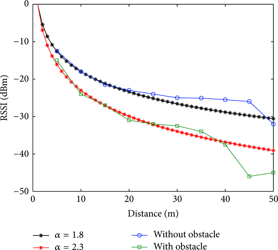
RSSI versus distance.

Outdoor Scenario Settings. Sensor nodes are randomly deployed in a fixed 100 m × 100 m square field by the Waxman random network topology generator [29]. The reason to choose the random deployment is that sensors are usually scattered randomly in the wild. The number of sensor nodes are varied between 20 and 60 to simulate different levels of density.

Indoor Scenario Settings. We use the real data trace from the 54 sensors deployed in Intel Berkeley Research lab, shown in Figure 9, monitoring the building environment information, such as temperature, light, humidity, and voltage values [30]. This data trace contains the aggregate connectivity data averaged over all time for 37 days, whose distribution and Cumulative Distribution Function (CDF) are shown in Figure 10. We establish the links with link quality above 0.5 in our indoor scenario simulations.

Figure 9

A deployment map of 54 sensors located in Berkeley lab.

Figure 10

Link quality of data trace. (a) Link quality distribution. (b) CDF of link quality.

Performance Metrics. We exploit the following metrics to evaluate the network performance. (1) Collection delay is measured as the time elapsed from packets being generated until all $(n-\mathrm{1})$ packets reach the sink, reported by the total number of time slots to complete data collection. (2) Energy consumption is measured by the total number of transmissions for all packets delivered to the sink. Since the power level is fixed, the power consumption of each transmission is equal. (3) Delivery ratio is measured as the ratio of successful transmission times compared to the total number of transmissions for all packets delivered to the sink.

Simulation Results

(1) Results in Outdoor Scenario. Each simulation is repeated for 100 times, and we report the average values as statistical results. In order to evaluate the impact of duty cycles, the duty cycles are set to be 0.05, 0.1, 0.15, 0.2, and 0.25, respectively. 40 nodes are randomly deployed in 100 × 100 square field. In order to show the improvement of time efficiency for eliminating all interfering links, RCTS is compared with MDCD-IL, which exploits extra time slots to eliminate interfering links. We present the results comparing our RCTS algorithm with MDCD-IL and the Dijkstra Algorithm as well as the upper and lower bounds on the data collection delay.

Figures 11 and 12 show the data collection delay and the number of transmissions under different duty cycles, respectively. From Figure 11, we can see that RCTS algorithm has the smallest delay than the compared Dijkstra Algorithm under different duty cycles while retaining low energy cost, since the number of transmissions remains small and stable over different duty cycles shown in Figure 12. As Figure 11 depicts, the delay of RCTS algorithm outperforms that of Dijkstra Algorithm by 32% to 11% when duty cycle increases from 0.05 to 0.25. Since the available time for nodes to receive packets is notably reduced, lower duty cycle has high probability to incur collisions. The channel and time scheduling of RCTS algorithm can largely reduce collisions, and the advantage of RCTS algorithm is more obvious in lower duty cycle. Compared with RCTS and MDCD-IL, we observe that the use of multiple channels can efficiently improve the data collection delay when the interfering links are avoided by multiple channels. It is also observed that the collection delay of RCTS algorithm almost overlaps its lower bound. Thus, it validates that RCTS algorithm can obtain the optimal solution.

Figure 11

Delay versus duty cycles.

Figure 12

Number of transmissions versus duty cycles.

From Figure 12, we find that the duty cycle has slight effect on the number of transmission in RCTS algorithm, which outperforms the Dijkstra Algorithm up to 67%. Figure 13 shows that the number of transmissions is positively correlated with the total number of nodes in the network, while little is related with the duty cycle. Thus, it is a good way to save energy by reducing the duty cycle, which will not cause increased transmission times. The reason is that RCTS algorithm is scheduled well without collision to retransmission. We can also infer that the delay in low-duty-cycle WSNs is mainly caused by sleep latency instead of retransmission.

Figure 13

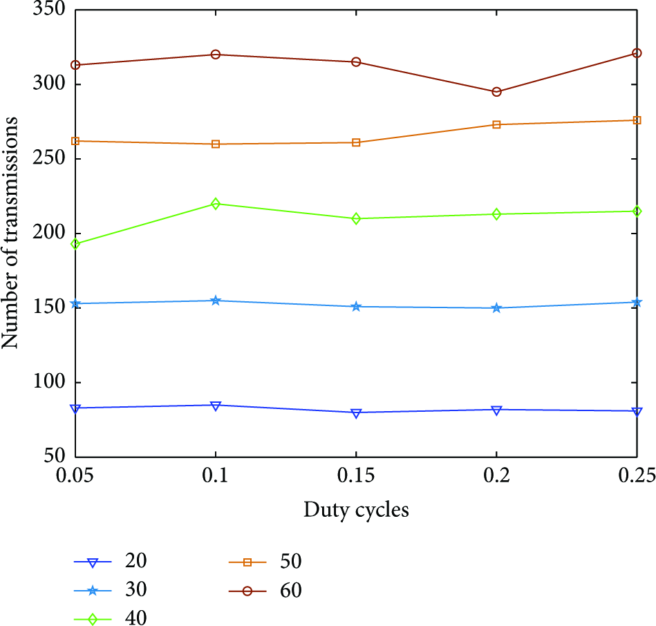
Number of transmissions versus duty cycles.

We use U and D to represent the upbound of collection delay and the time distance from the upbound to the optimal latency, respectively. We define the ratio of D and U to evaluate the effectiveness of RCTS algorithm. From Figure 14, we also find that the effectiveness of RCTS algorithm has little impact on the number of nodes and duty cycle and stays between the range of 30% and 50%.

Figure 14

The effectiveness of RCTS algorithm under different cases.

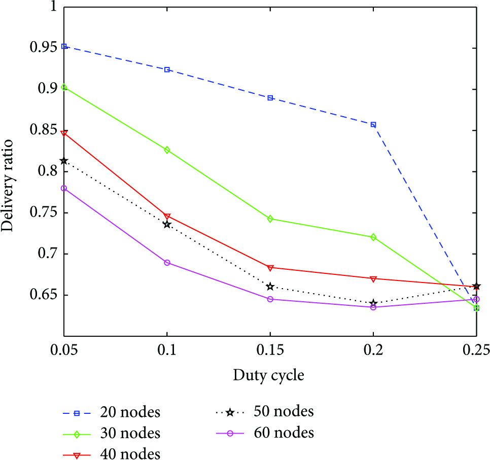
From Figure 15, we can observe that the delivery ratio raises rapidly, when the duty cycle decreases to 0.2. The concurrent transmissions on the same channel are alleviated, since the probability of nodes active simultaneously is reduced. When the duty cycle is extremely low (less than 0.1), we observe that the single channel is enough to deliver packets with few interfering links as the deployment gets sparser (less than 0.4). This happens because at low densities the interference is less and less concurrent transmissions take place. We also find that the delivery ratio can be over 0.9 when the duty cycle and density are both low, which can satisfy the requirements in most wireless networks.

Figure 15

Delivery ratio under different duty cycle.

Figure 16 shows the number of assigned channels by Algorithm 3 with different node densities when the duty cycle is set to be 0.25. With the increase of node density, the channel resources are needed more to eliminate the interfering links. As we can see from Figure 16, when the number of nodes augments to 60, we need at most 13 channels to avoid interfering links. We find that channel scheduling can suffice to eliminate most interference for moderate size of about 60 nodes in the outdoor environment, even when the duty cycle is not extremely low (0.25).

Algorithm 3: Receiver-based Channel and Time Scheduling algorithm.

Input: The original network topology.

Output: The optimal data collection paths and channel assignment

with the minimum delay.

(1) Call the DFDC algorithm to obtain the optimal link

  schedule on the same channel.

(2) The receivers check the SINR condition among the concurrently

 transmitting senders

(3) if There exist receivers with $$\text{SINR}\le \beta$$   then

(4)   The receiver with lower $$p(i)$$ assigns one available

    channel.

Figure 16

Occupied channels distribution.

(2) Results in the Indoors Scenario. We also use the exponential path-loss model for signal propagation with the path-loss exponent α varying between 3 and 4, which is typical for the indoor environment. Based on the physical interference model, the transmission power is also set to be the highest level and SINR threshold is set as $\beta =-\mathrm{3}$  dB. The above parameters setting is the same as [24].

From Figure 7, we see that the delivery ratio is relatively high when all nodes communicate on the same channel in the indoor environment. Since the signal strength rapidly degrades with the increase of communication distance, the interference among neighbors will decrease accordingly. Thus, the appearance of interfering links will reduce in large amount. Although the delivery ratio of CFDC algorithm is in good performance, in order to ensure the stable communication, we can also use the multichannel scheduling to improve the performance of CFDC algorithm further. Figure 17 shows the mean number of assigned maximum channels in different path-loss exponent (α) by Algorithm 3. The performance improvement of RCTS is more obvious when the duty cycle is highly compared with CFDC algorithm.

Figure 17

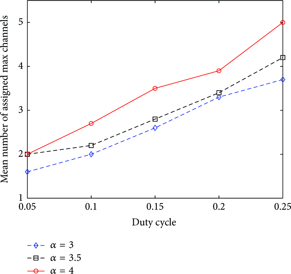
Number of channels versus duty cycles.

8. Conclusion

In this paper, we studied the problem: How fast can raw data be collected from all source nodes to a sink in low-duty-cycle WSNs with general topology? Both lower and upper tight bounds were given for this problem. We presented both centralized and Distributed Fast Data Collection algorithms to address this problem, both of which are able to find an optimal solution in polynomial time when no interfering links happen. When interfering links happen, multichannel scheduling is introduced to eliminate the interfering links. We next proposed a novel Receiver-based Channel and Time Scheduling (RCTS) algorithm to obtain the optimal solution. Based on real trace, extensive simulations were conducted and the results showed that the proposed distributed RCTS algorithm is significantly more efficient than the link schedule on the same channel and achieved the lower bound. We also evaluated the multichannel scheduling method and found that multichannel scheduling can suffice to eliminate most of the interference in both the indoor and outdoor environment for moderate size networks. In the future, we shall extend this work into the case of unreliable links.