Sage Journals: Discover world-class research

Abstract

Mobile charge problem describes a fleet of mobile chargers delivers energy to the sensor nodes periodically in wireless sensor networks (WSNs). In it, every sensor node has an asynchronous rest working time during a charging round. We consider the asynchronous rest working time and give the lower and upper bounds of the recharging cycle by the suitable total serving rate, to give the definition of time windows for the sensor nodes. In this paper, we model this problem in 2-dimensional WSNs as a vehicle routing problem with time windows (VRPTW). For solving the problem of multiple mobile chargers with different routing paths, we propose to transform the multiple routing problems into a single routing problem, by duplicating the sink into multiple virtual sinks. To optimize the routing path, we propose a local optimization algorithm by considering the collaborative charging among the mobile chargers. Through the simulations, we compare our proposed algorithm with the $H η C l u s t e r C h a r g i n g (β)$ algorithm. We demonstrate the advantages of our collaborative scheduling algorithm in this problem.

1. Introduction

Recent breakthroughs in wireless energy transfer and rechargeable lithium batteries provide a promising support for the energy problem of WSNs. Experimental demonstration in [1] shows the energy can be efficiently transmitted between magnetically resonant objects without any conduction. Rechargeable lithium batteries own high energy densities and high charge capabilities as shown in [2].

Supported by these enabling technologies [3–5], some studies envisioned employing a mobile vehicle which carries a high volume battery as a mobile charger to periodically deliver energy to the sensor nodes. Minimizing the tour length of each mobile vehicle is a critical challenge because of its NP-hard property. Moreover, the total delay time above their energy threshold is also positive correlation with tour length while the velocity of mobile charger is fixed. The works in [6, 7] focused on minimizing the tour length and total delay time, respectively.

However, most of them assumed that a sensor node can be charged as long as its energy is consumed. It is obviously that charging a sensor node one time with the energy of $B / 2$ energy (B is the sensor capacity) is more effective than charging a sensor twice with the enery of $B / 4$ . Thus, it is reasonable to give an upper bound of residual energy which means it is unnecessary to be charged when a sensor's residual energy is larger than this upper bound. Combined with upper bound of energy and lower bound of energy (energy is exhausted), Louafi et al. in [8] consider the battery capacity of chargers and give his collaboration algorithm $H η C l u s t e r C h a r g i n g (β)$ to deal with the energy constraint of the mobile charger. However, it may overlook the emergency situation when the number of sensor nodes, whose residual energy is under threshold value, are larger than charger number.

This problem can be described in detail as follows. WSNs, for all sensor nodes in WSN, own their time windows based on their residual energy. Our problem is to schedule a fleet mobile chargers, which have same battery capacity and velocity, to charge all sensor node in WSNs and back to charger station. The objective is to maximize the total energy level after one process of charging.

In this paper, we consider the prior studies and give our specific mobile charge problem as vehicle routing problem with time windows (VRPTW) with combining the problem of minimizing the tour length and time windows of the sensor nodes. We consider optimizing the total energy level after charging the WSNs one time. We add virtual charger station based on the number of the chargers and then transform the problem into a Hamilton cycle problem. The number of the chargers can be obtained based on the quantitative relationship of charger's property parameter. Then, we optimize the Hamilton cycle via specific local optimization and collaboration among mobile chargers.

The rest of our paper is organized as follows. Some related works are presented in Section 2. The problem formulation is given in Section 3. Section 4 presents our schedule scheme, and Section 5 evaluates it through simulations. Finally, Section 6 summarizes the paper and outlines the research perspectives.

2. Related Work

Many prior works prolong the lifetime of WSNs that supported and inspired our basic idea. We describe a subset of these related efforts in this section.

Supporting Technology. Energy harvesting extracts environmental energy to complements sensor nodes. Cammarano et al. [9] and Kansal and Srivastava [10] proposed energy prediction model for environment energy efficient utility. Voigt et al. [11] proposed solar aware routing manner. These works are showing great promise of addressing the energy problem in WSNs. Bhattacharya et al. [12], Wang et al. [13], and Dunkels et al. [14] consider energy conservation for slowing down energy consumption rate, but it cannot compensate for depletion. It may be efficient for combining the energy conservation and chargers' scheduling.

Existing Energy Transfer Algorithm. Peng et al. [15] and Li et al. [16] focused on maximizing network lifetime through finding an optimal charging sequence. Shi et al. [6] assumed that the mobile charger has unbounded energy and investigated the problem of periodically charging sensors to maximize the ratio of the chargers vacation time (time spent at the home service station) over the cycle time. They further considered the multinode simultaneous charging scenario [17, 18]. Fu et al. [7] focused on minimizing the total delay of replenishing all sensor nodes in a network. Louafi et al. [8] focused on maximizing the energy usage effectiveness through collaborate among chargers. These motivation related works born our specific problem VRPTW, to maximize the residual energy rate.

Before we give our problem formulation, we firstly give the general problem definition of mobile charging problem [8]. In general problem, they define the problem model as WSNs model with parameter X Y B T and define the solution model as charge model with parameter $(P, c, v, η_{1}, η_{2})$ , where X and Y combine the location of node s, $(x_{i}, y_{i} | x_{i} \in X, y_{i} \in Y)$ . B is the sensor capacity set and T is the recharging cycle set of sensors. The charge model: for every charger, the battery capacity is P, the travelling speed is v, energy consumed by travelling one unit distance is c, $η_{1}$ is the charging efficiency between a charger and a sensor node, and $η_{2}$ is the charging efficiency among chargers. In order to unify with general problem, we also call the charger station as base station.

3. Problem Formulation

The general mobile charge problem was described as WSNs( $X, Y, B, T$ ) model and charge model $(P, c, v, η_{1}, η_{2})$ [8], and we also describe our problem as WSNs model and charge model. In this section, we will illustrate the difference between our specific mobile charge problem and general mobile charge problem one by one. Then, we explain the reason why we choose specific like this.

3.1. Our Mobile Charge Model

We first give our specific mobile charge model: WSNs $(V, E, B, R, TW, D)$ and $(M, P, c, v, η_{1})$ , where $V = {v_{0}, v_{1}, v_{2}, \dots, v_{n}}$ is sensor nodes set and $v_{i}$ represents the ith sensor node, and $v_{0}$ denotes the base station especially. $E = {d_{i j} = (v_{i}, v_{j}) | v_{i}, v_{j} \in V}$ is the weight set where $d_{i j}$ represents the Euclidean Distance from $v_{i}$ to $v_{j}$ . Node and weight sets V, E tell us the distribution of wireless sensor networks, and we can know the sensors residual energy and energy consuming rate by $B = {b_{1}, b_{2}, \dots, b_{n}}$ and $R = {r_{1}, r_{2}, \dots, r_{n}}$ (every sensor node has different residual energy and energy consuming, and we will explain the reason following). The following charge model is similar to the general mobile charge problem: M mobile chargers are homogeneous, and for every charger, the battery capacity is P, the travelling speed is v, energy consumed by travelling one unit distance is c, and $η_{1}$ is the charging efficiency between a charger and a sensor node. Both travelling and wireless charging share the same battery on a mobile charger.

It is easy to find that $TW$ and D are the additional conditions in our model, where $TW$ is the time windows set for every nodes and D is the radius of the wireless sensor networks (we assume the WSNs as a circular area and sensor nodes distribute in this region).

3.2. Reasons of Our Specific Mobile Charge Problem

Before explaining the difference between our specific problem and the general problem, we give three practical conditions of WSNs and two assumptions.

There are three practical conditions. (1) If we need schedule mobile chargers to charge the WSNs frequently in a short time, it may be more reasonable to partition all sensor nodes into several groups and place a charge station at the center of each group to charge these sensors in the group periodic by wireless charge. (2) Each node consumes energy for sensing, data reception, and transmission. These processes frequently occur conducted by events they monitor which are obeying different parament value of exponential distribution in different environments. (3) The charge station gets the residual energy information of all sensor nodes before schedule mobile chargers to charge the WSNs.

There are two assumptions. (1) Short duration (SD): the duration of a charging is negligible compared to the traveling time of mobile chargers. (2) Long cycle (LC): the recharging cycle of a sensor node is longer than a charging round (it means any two consecutive charging rounds have no intersections). It is easy to find that these assumptions can be explained by practical condition (1).

3.2.1. Different Energy Consuming Rate

The work [19] aims at scheduling the work sequencing of sensor nodes to maximize the time of sustaining the WSNs work due to the condition (2). So, the energy consuming rate of each sensor node in WSNs is different in different environments according to the work addressed in [19].

3.2.2. Time Windows

With the assumption of long cycle (LC), the mobile charge problem focuses on a random time during a recharge cycle when some sensor nodes exhausted. Due to the different energy consuming rate, the residual energy of all sensor nodes must be not common when charge station decides to schedule mobile chargers. With an intuitive observation that charging a sensor node one time with $2 q$ energy must be more effective than charging a sensor node q energy twice in a periodic. So we assume to charge a sensor node while its residual energy is less than $b_{low}$ . And this is also the result of the assumption of LC, when you charge a sensor node with a residual energy larger than $b_{low}$ , and the energy may keep the sensor node working without recharge in several charging rounds and still with residual energy larger than $b_{low}$ . All of this, we give the time windows $TW = {[l_{1}, u_{1}], [l_{2}, u_{2}], \dots, [l_{n}, u_{n}]}$ of all sensor nodes which mean a mobile charger must charge sensor node $v_{i}$ during time interval $[l_{i}, u_{i}]$ .

3.2.3. Radius of WSNs

Under a determined charge model $(M, P, v, c, η_{1})$ , it is obviously that mobile chargers cannot serve the sensors distribution at bordering of the WSNs while the radius of WSNs is too large. There exists quantitative relationship between the radius of WSNs and the paraments of charge model $(M, P, v, c, η_{1})$ .

3.3. Number of Mobile Charger

The paper [20] has presented a method to estimate the number of mobile chargers. However, its hypothesis differs from our problem. Thus, we give our quantitative relationship of mobile charger number M.

Then, we give the low bound of mobile charger number. A clear understanding of relationship between mobile charger number M and mobile charger routing is that the better schedule of mobile charger, the less number of mobile charger necessary. So, it may be impossible to give an accuracy mobile charger number before scheduling the routing. An extreme situation is that mobile charger number M is equal to sensor node number n. Another challenge to give the mobile charger number is the constraint of time windows. Several sensor nodes cannot be served by one mobile charger in time because of their location distribution. So, we give an approximation of lower bound of M with these two aspects.

For Energy Consumption. First, we estimate the lower bound of M through the perspective of energy consumption. The energy consumed in replenishing a WSN contains two parts: the energy charging to sensors and the energy consumed by chargers' travelling. Although it is hard to exactly get the length of travelling distance, we can give the mean of all edges $d = (1 / n^{2}) \sum_{i = 1}^{n} ‍ \sum_{j = 1}^{n} ‍ d_{i j}$ to represent the average length of one edge in travelling when we know the mobile charger number:

\begin{matrix} M \cdot P \geq c (n_{1} + M) \cdot d + \frac{1}{η_{1}} \sum_{k = 1}^{n_{1}} ‍ (b - b_{σ_{k}}), \\ M \geq M^{e c} = \frac{n_{1} d c + (1 / η_{1}) \sum_{k = 1}^{n_{1}} ‍ (b - b_{σ_{k}})}{P - d \cdot c} . \end{matrix}

(1)

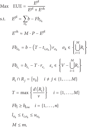
This is just an approximation of lower bound $M^{e c}$ and larger than the real lower bound from the perspective of energy consumption.

3.4. Objective Function and Constraints

Now, we give the mathematical description of our specific mobile charge problem including objective function and constraints.

In a scheduling cycle, the energy consumed in replenishing a WSNs contains three parts: the energy eventually obtained by sensors, the energy consumed by chargers' travelling, and the energy loss during charging. The 1st part is defined as payloadenergy ( $E^{pl}$ ), and the sum of the 2nd and 3rd parts is defined as overheadenergy ( $E^{oh}$ ). The energy usage effectiveness (EUE) is defined as

\begin{matrix} EUE = \frac{E^{pl}}{E^{pl} + E^{oh}} . \end{matrix}

(2)

So far, we can give our brief mathematic model of this specific problem according to the above analysis result as 2.

We can describe our specific mobile charge problem as a selective vehicle routing problem with time windows. When the charger station schedules M mobile chargers simultaneously, charge all sensor nodes whose energy residual is lower than $b_{low}$ (we call these nodes as desire nodes) and all chargers back to base station when all sensor nodes' residual energy is larger than $b_{low}$ (formulated as the fifth equation in constraints). The fourth equation in constraints is the time in which the fleet mobile chargers serve the WSNs. Just because of the constraint of serve time, some sensor nodes may consume their energy lower than $b_{low}$ during the serve time. So we call these sensor nodes as hidden nodes. Desire nodes and hidden nodes combine the serving sensor nodes ${σ_{1}, σ_{2}, \dots, σ_{k}, \dots, σ_{n_{1}}}$ which mobile chargers need to serve. Left sensor nodes ${ε_{1}, ε_{2}, \dots, ε_{s}, \dots, ε_{n_{2}}}$ are unnecessary to serve by mobile chargers, and $n_{1} + n_{2} = n$ . So we can find the first and second equations in constraints denoting the eventual residual energy of serving sensor nodes and rest sensor nodes, respectively. The third equation in constraints means every sensor node from desire nodes set is only charged by one mobile charger one time. The last two equations in constraints are as follows: every desire sensor node must be served during time windows and give the upper bound of mobile charger number. The correct expression of m will be given in the next section:

\begin{array}{l} Max EUE = \frac{E^{pl}}{E^{pl} + E^{oh}} \\ s . t . E^{pl} = \sum_{σ_{k}} ‍ b - F b_{σ_{k}} \\ E^{oh} \approx M \cdot P - E^{pl} \\ F b_{σ_{k}} = b - (T - t_{i, σ_{k}}) r_{σ_{k}} σ_{k} \in \{⋃_{i = 1}^{M} ‍ R_{i}\} \\ F b_{ε_{s}} = b_{ε_{s}} - T \cdot r_{ε_{s}} ε_{s} \in \{V - ⋃_{i = 1}^{M} ‍ R_{i}\} \\ R_{i} \cap R_{j} = {v_{0}} i \neq j \in {1, \dots, M} \\ T = \max \{\frac{d (R_{i})}{v}\} i = {1, \dots, M} \\ F b_{i} \geq b_{low} i = {1, \dots, n} \\ l_{σ_{k}} \leq t_{i, σ_{k}} \leq u_{σ_{k}} \\ M \leq m, \end{array}

(3)

where

F b_{σ_{k}}

is the final residual energy of

σ_{k}

th sensor node.

4. Our Scheduling Algorithm

In this section, the scheduling algorithm will be given to solve our specific problem when WSNs model and charge model are determined with the above analysis.

4.1. Adding Virtual Node

Our specific problem can be translated into a vehicle routing problem with time windows (VRPTW). We perform this transform to improve the quality of solution and do local optimization after building solution, because the single routing problem is easier than multiple routing problem. So, we translate our multiple routing problem into single routing problem through adding virtual charger station. Figure 1 explain the processing intuitively.

Figure 1

Translation of the virtual nodes.

The left figure in Figure 1 is the initial routing, and the right figure is the routing after transform. The addition two charger stations (square) are virtual node, and it means a mobile charger arrives charger station in practical when it arrives virtual node in figure (the distance among virtual node and other sensor nodes is equal to the distance among charger station and other sensor nodes). With this transform, in our specific problem the left figure in Figure 1 is translated into Hamilton cycle that each node in graph must be visited if and only if one time. This transform is also prepared for the local optimization in Section 4.3.

4.2. Main Rules of Our Algorithm

To build a feasible routing which satisfied time windows and energy constraint, we design some building rules as follows.

First, we build a candidate set to provide mobile charger selecting a suitable sensor node to charge according to its current residual energy and time. $P_{c}$ and $T_{c}$ are the current residual energy and current time of a charger. A sensor $v_{i}$ belonging to a charger's candidate set $V_{candi}$ when the charger's residual energy can provide the charger move from its current node to $v_{i}$ charging it and back to base station. Another constraint is that the charger must arrive to $v_{i}$ during the $v_{i}$ time windows. So we give the following candidate set:

\begin{matrix} V_{candi} = \{v_{i} | P_{c} > \frac{b_{i}}{η_{1}} + c (d_{c i} + d_{i 1}), l_{i} < T_{c} + \frac{d_{c i}}{v} < u_{i}\}, \\ V_{candi} \cap V_{visited} = \{\emptyset\}, \end{matrix}

(4)

where 4 is candidate set while mobile charger has already charging a set of sensor nodes

V_{visited}

and arrive at

v_{c}

. And the candidate set

V_{candi}

must no intersection with visited node set

V_{visited}

When the candidate set $V_{candi} = {\emptyset}$ , the mobile charger must return back to base station. We will give the pseudocode of our algorithm in Algorithm 1.

Algorithm 1: Schedule algorithm for VRPTW.

Require: WSNs model ( $V, E, B, R, TW, D$ ) and Charge Model ( $M, P, v, c, η$ );

Ensure: State variables current time $T_{c}$ and current energy $E_{c}$ , current routing sequence R.

(1) for $i = 1$ ; $i \leq n + M$ ; $i + +$ do

(2) calculate unvisited sensor nodes set $V_{unvisited}$ with current sequence $R = {r_{1}, r_{2}, \dots, r_{i - 1}}$ ;

(3) calculate feasible sensor nodes set $V_{tw}$ about time windows with current time $T_{c}$ ;

(4) calculate feasible sensor nodes set $V_{ec}$ about energy constraint with current energy $E_{c}$ ;

(5) obtain the candidate feasible sensor nodes set $V_{candi} = V_{unvisited} \cap V_{tw} \cap V_{ec}$ ;

(6) if $V_{candi} \neq \emptyset$ then

(7) $r_{i} = \underset{j \in V_{candi}}{argmin} {d_{r_{i - 1}, j}}$ ;

(8) Add $r_{i}$ to R;

(9) Refresh paraments about $T_{c}$ , $E_{c}$ ;

(10) else

(11) $r_{i} = BaseStation$ ;

(12) Add $r_{i}$ to R;

(13) Refresh paraments about $T_{c} = 0$ , $E_{c} = P$ ;

(14) end if

(15) end for

(16) Using collaboration to optimize the solution R.

(17) Calculate the objective function EUE.

With the transform in Section 5.1, the algorithm can be regarded as a greedy algorithm to solving a constraint $TSP$ problem. $n + M$ is the number of total node and with $M - 1$ virtual nodes. Line 2–5 obtains the candidate set in step i according to history routing and current residual energy and current time. Adding the nearest node in routing and refresh $T_{c} = T_{c} + d_{r_{i - 1}, r_{i}} / v$ , $E_{c} = E_{c} - d_{r_{i - 1}, r_{i}} \cdot c - (B - b_{i}) - r_{i} \cdot T_{c}$ if the candidate set is not empty, otherwise, refresh the current $T_{c} = 0$ , $E_{c} = P$ . After $n + M$ steps (line 1–15), the solution has built and did some improvement (line 16-17).

4.3. Collaboration between Mobile Charger

Finally, we use collaboration among mobile chargers to optimize the solution.

After we built a feasible routing and using 2-opt to improve the tour, we consider whether we should improve the solution further more. Such as the left picture in Figure 2, the routing $i \to i + 1, \to, \dots$ crosses with routing $j \to j + 1, \to, \dots$ . We can improve it like the right picture, but the feasibility of the change must be kept. This improvement is based on the wireless energy transfer and collaboration of chargers.

Figure 2

Processing of collaboration.

4.4. The Complexity of Algorithm

In Algorithm 1, lines 2–4 are the processes to calculate node sets. All of them are finishing in linear time $O (n)$ . In lines 6–14, line 7 is linear time complexity $O (n)$ , and the rest processes are constant complexity $O (1)$ . And the process in lines 16-17 is at most $O (n^{2})$ . Thus, the total time complexity is $O (n^{2})$ .

5. Performance Evaluation

Three different simulations would be done in this section, and we will give the analysis in detail.

5.1. Simulation Setup and Quantitative Check

We assume that sensor nodes are powered by a 1.5 V 2000 mAh Alkaline rechargeable battery, and then the battery capacity $(b)$ is $1.5 V \times 2 A \times 3600 sec = 10.8 KJ$ ; the battery capacity of a mobile charger $(P)$ is 2000 KJ, and moving speed of charger $(v)$ is 1 m/s; the charger's moving cost $(c)$ is 10 J/m. With the analysis of Section 4, we first give the size of WSNs $D = (b \cdot v) / (1.5 V \times 2 A / 2)$ , and this is based on the limitation of sensor battery capacity and charger velocity. We assume that wirless sensor nodes are uniformly deployed over a $[- D \times D]$ 2-dimensional square area. The base station $B S$ is located at the center of the square, and the coordinates of $B S$ are (0,0). By default, the number of sensor nodes $(N)$ is set 200. After determining the location of a sensor node $v_{i}$ , we can know the energy consuming rate $r_{i}$ . We assume $b_{i} = ⋃_{} ‍ [d_{1 i} r_{i} / v, b]$ , with a given $q_{1}$ and $q_{2}$ , and we can obtain $b_{low}$ by 4. So that, we can give the lower and upper bounds of sensor node $v_{i} [l_{i}, u_{i}]$ by 3. Another way of simulation setup: if we have already known the mobile charger number M, we can give the size of WSNs D by 1 and the rest parameters can be given the same as above. With the setup above, we can keep our words that the WSNs model can be charged by charge model feasibly.

We compare our $S c h e d u l e A l g o r i t h m$ with $H η C l u s t e r C h a r g i n g (β)$ algorithm and their improvement, $S c h e d u l e A l g o r i t h m + 2 o p t$ , $H η C l u s t e r C h a r g i n g (β) + 2 o p t$ , and $^{'} + 2 {o p t}^{'}$ , means we are adding a local search algorithm called “2opt” [21] in this algorithm again. We compare these four algorithms through residual energy rate, mobile charger number, and feasible node rate, respectively.

5.2. Compare Results in Energy Usage Effectiveness

Figure 3 expresses the EUE value with these four algorithms when sensor number, battery capacity of a charger, battery capacity of sensor node and moving cost of a charger changed. An obvious look is that algorithm with “2opt” is better than the algorithm simply and improvement of “2opt” on ScheduleAlgorithm is limited. It is because our algorithm ScheduleAlgorithm has already improved by local optimization and collaboration. With the result of Figure 3, our ScheduleAlgorithm is better than the HηClusterCharging $(β)$ algorithm on EUE.

Figure 3

Performance comparisons for EUE.

In Figure 3(a), when the number of sensor nodes increases, mobile chargers may cost more time to finish a charging round; this means more energy would be cost by sensor nodes. According to this, all of the four algorithms perform worse when the number of sensor nodes decreases. A few wave will be shown because of the specificity of every example. In Figure 3(c), as the battery capacity of a sensor node increases, the EUE of all four algorithms also increases. This is reasonable, since charger can deliver more energy to a sensor node in one cycle. In Figures 3(b) and 3(d), the EUE is not changed with the increase of charger battery capacity and moving cost. It is because, there is no relevant among the variables EUE, moving cost and battery capacity. As the battery capacity of charger increases, it may decrease the charger number we used to charge, but it still cannot decrease the maximum travelling time of mobile chargers. So, there is no change for EUE with the increase of charger battery capacity.

6. Conclusion

In this paper, we investigate the mobile charging scheduling problem in WSNs. By introducing energy charging bound, we translate the problem into classic problem vehicle routing problem with time windows (VRPTW). We add M virtual base stations to translate the multiple routing problem into single routing problem and use local optimization and collaboration to optimize the solution. And the results of simulation validate the advantages of our algorithm.

Footnotes

Conflict of Interests

The authors declare that there is no conflict of interests regarding the publication of this paper.

References

Kurs

Karalis

Moffatt

Joannopoulos

J. D.

Fisher

Soljačić

Wireless power transfer via strongly coupled magnetic resonances

The American Association for the Advancement of Science. Science 2007 317 5834 83 86

10.1126/science.1143254

MR2335122

2-s2.0-34447309715

Kang

Meng

Y. S.

Bréger

Grey

C. P.

Ceder

Electrodes with high power and high capacity for rechargeable lithium batteries

Science 2006 311 5763 977 980

10.1126/science.1122152

2-s2.0-33244474899

Dai

Dong

Chen

Impact of mobility on energy provisioning in wireless rechargeable sensor networks

Proceedings of the IEEE Wireless Communications and Networking Conference (WCNC '13)

April 2013

962 967

10.1109/WCNC.2013.6554694

2-s2.0-84881569322

Al-Karaki

J. N.

Kamal

A. E.

Routing techniques in wireless sensor networks: a survey

IEEE Wireless Communications 2004 11 6 6 27

10.1109/MWC.2004.1368893

2-s2.0-11144277843

Potdar

Sharif

Chang

Wireless sensor networks: a survey

Proceedings of the IEEE International Conference on Advanced Information Networking and Applications Workshops (WAINA '09)

May 2009

636 641

10.1109/WAINA.2009.192

2-s2.0-70350104731

Shi

Xie

Hou

Y. T.

Sherali

H. D.

On renewable sensor networks with wireless energy transfer

Proceedings of the IEEE (INFOCOM '11)

April 2011

Shanghai, China

1350 1358

10.1109/INFCOM.2011.5934919

2-s2.0-79960889049

Cheng

Chen

Minimizing charging delay in wireless rechargeable sensor networks

Proceedings of the 32nd IEEE Conference on Computer Communications (INFOCOM '13)

April 2013

2922 2930

10.1109/INFCOM.2013.6567103

2-s2.0-84883080417

Louafi

Coulombe

Chandra

Quality prediction-based dynamic content adaptation framework applied to collaborative mobile presentations

IEEE Transactions on Mobile Computing 2013 12 10 2024 2036

2-s2.0-84883143873

10.1109/TMC.2012.173

Cammarano

Petrioli

Spenza

Pro-Energy: a novel energy prediction model for solar and wind energy-harvesting wireless sensor networks

Proceedings of the 9th IEEE International Conference on Mobile Ad-Hoc and Sensor Systems (MASS '12)

October 2012

Las Vegas, Nev, USA

75 83

10.1109/MASS.2012.6502504

2-s2.0-84877659567

10.

Kansal

Srivastava

M. B.

An environmental energy harvesting framework for sensor networks

Proceedings of the International Symposium on Low Power Electronics and Design (ISLPED '03)

August 2003

481 486

2-s2.0-1542359103

11.

Voigt

Ritter

Schiller

Utilizing solar power in wireless sensor networks

Proceedings of the 28th Annual IEEE International Conference on Local Computer Networks (LCN '03)

October 2003

416 422

10.1109/LCN.2003.1243167

12.

Bhattacharya

Kim

Prabh

Abdelzaher

Energyconserving data placement and asynchronous multicast in wireless sensor networks

Proceedings of the 1st International Conference on Mobile Systems, Applications and Services

2003

ACM

173 185

13.

Wang

Srinivasan

Chua

K.-C.

Using mobile relays to prolong the lifetime of wireless sensor networks

Proceedings of the 11th Annual International Conference on Mobile Computing and Networking (MobiCom '05)

September 2005

ACM

270 283

2-s2.0-32144461553

14.

Dunkels

Österlind

An adaptive communication architecture for wireless sensor networks

Proceedings of the 5th ACM International Conference on Embedded Networked Sensor Systems (SenSys '07)

November 2007

335 349

10.1145/1322263.1322295

2-s2.0-79959879300

15.

Peng

Zhang

Qiao

Prolonging sensor network lifetime throughwireless charging

Proceedings of the 31st IEEE Real-Time Systems Symposium (RTSS '10)

December 2010

IEEE

129 139

10.1109/RTSS.2010.35

2-s2.0-79951799759

16.

Peng

Zhang

Qiao

Study of joint routing and wireless charging strategies in sensor networks

Wireless Algorithms, Systems, and Applications 2010 6221

Berlin, Germany

Springer

125 135 Lecture Notes in Computer Science

10.1007/978-3-642-14654-1_17

17.

Xie

Shi

Hou

Y. T.

Lou

Sherali

H. D.

Midkiff

S. F.

On renewable sensor networks with wireless energy transfer: the multi-node case

Proceedings of the 9th Annual IEEE Communications Society Conference on Sensor, Mesh and Ad Hoc Communications and Networks (SECON '12)

June 2012

10 18

10.1109/SECON.2012.6275766

2-s2.0-84867922457

18.

Chen

Jiang

Yau

D. K. Y.

Xing

Sun

Energy provisioning in wireless rechargeable sensor networks

IEEE Transactions on Mobile Computing 2013 12 10 1931 1942

2-s2.0-84883113038

10.1109/TMC.2012.161

19.

Dai

Chen

Practical scheduling for stochastic event capture in wireless rechargeable sensor networks

Proceedings of the IEEE Wireless Communications and Networking Conference (WCNC '13)

April 2013

IEEE

986 991

10.1109/WCNC.2013.6554698

2-s2.0-84881599274

20.

Wang

Yang

Multi-vehicle coordination for wireless energy replenishment in sensor networks

Proceedings of the 27th IEEE International Parallel and Distributed Processing Symposium (IPDPS '13)

May 2013

Boston, Mass, USA

1101 1111

10.1109/IPDPS.2013.22

2-s2.0-84884870482

21.

Mou

L.-M.

Dai

X.-L.

A novel ant colony system for solving the one-commodity traveling salesman problem with selective pickup and delivery

Proceedings of the 8th International Conference on Natural Computation (ICNC '12)

May 2012

Chongqing, China

1096 1101

10.1109/ICNC.2012.6234622

2-s2.0-84866154384

Scheduling with Collaborative Mobile Chargers Inter-WSNs

Abstract

1. Introduction

2. Related Work

3. Problem Formulation

3.1. Our Mobile Charge Model

3.2. Reasons of Our Specific Mobile Charge Problem

3.2.1. Different Energy Consuming Rate

3.2.2. Time Windows

3.2.3. Radius of WSNs

3.3. Number of Mobile Charger

3.4. Objective Function and Constraints

4. Our Scheduling Algorithm

4.1. Adding Virtual Node

4.2. Main Rules of Our Algorithm

Algorithm 1: Schedule algorithm for VRPTW.

4.3. Collaboration between Mobile Charger

4.4. The Complexity of Algorithm

5. Performance Evaluation

5.1. Simulation Setup and Quantitative Check

5.2. Compare Results in Energy Usage Effectiveness

6. Conclusion

Footnotes

Conflict of Interests

References