Parameter Optimization of a Temperature and Relative Humidity Based Transmission Power Control Scheme for Wireless Sensor Networks

Abstract

We present refinements of a novel transmission power control (TPC) algorithm based on temperature and relative humidity (TRH). Previously, we deployed a prototype TRH TPC algorithm on wireless sensor nodes operating in real harsh environmental conditions and reported promising results. Since then, we have made enhancements of the TRH TPC model, which we will show here. Furthermore, in order to develop an understanding of the nonlinear behavior that we observed from this TRH TPC scheme, we developed a simulation platform that uses real radio frequency (RF) signal and interference samples and actual T and RH sensor data acquired simultaneously. Afterwards, we logged results of repeated experiments and determined the algorithms operating ranges and behaviors, varying its main parameters, such as (1) its gain factor, (2) the average time period to recalculate power level updates, and (3) proper received signal threshold selection. We then summarize optimal parameter ranges from the analytical results that reflect where this TRH TPC technique works best. And finally, we report results of the TRH TPC algorithm running on long range WSN systems deployed in harsh environmental conditions, corroborating behaviors observed through simulation.

1. Introduction

There are many proposed transmission power control algorithms for wireless communications [1–3]; they vary according to what performance indicator they use to do power compensation; it depends on the selected wireless technology. The most commonly used wireless performance metric is the received signal strength indicator (RSSI), which is available on most commercial radios. Others use a metric called the link quality indicator (LQI) that comes with radios that deploy a type of modulation that breaks apart data bits in so-called “chips” and scatters them within the operating frequency band with the aim of mitigating interference [4, 5]. At the destination, the receiver tries to determine one data bit at a time by putting together the corresponding “chips.” The easier is the demodulation process for the receiver, the higher is the LQI it reports. In a sense, the LQI is a measure of the “chip error rate.” Another metric is called packet reception rate (PRR); it is stochastic in nature based on medium to long term averages and takes some time to be reliable.

Different TPC schemes operate at different layers. Some TPC proposals work at the medium access control (MAC) layer using the bit error rate (BER) metric [6]; others run in a cross layer manner involving routing tables [7]. The most studied approaches are adaptive techniques. They take into account the received signal power least mean squared (LMS) error, which needs a training phase that may take extended periods of time until actual compensation starts [8].

In a more recent article, authors of [9] deal with TPC using an active fade margin, which takes advantage of the well known path loss and power budget wireless link analysis; this scheme has the drawback that it needs to always have knowledge of the current channel noise floor level. Other publications show that the increase in temperature affects negatively the RSSI values. Bannister et al. in [10] measured the effect of temperature on the resulting RSSI levels, using two directly connected wireless nodes, via a coaxial cable with an attenuator between them to emulate distance. The nodes were exposed to infrared lamps to generate heat over them. From the results, they inferred a linear approximation within the 25°C to 65°C range. Nevertheless, these experiments were not done in a wireless manner because they used a coaxial cable; they only focused on loss due to temperature, ignoring other factors such as air humidity and RF interference, which may play a role in signal fading. Moreover, Lee and Chung in [11] accepted this claim and deployed an open loop temperature dependent TPC, using the linear expression proposed by Bannister.

Boano et al. in [12] also confirm Bannister's claims, but they go further by proposing an expression that describes a temperature dependent signal to noise ratio formula. Boano et al. in [13], through a set of experiments in an Italian wheat field, exposed wireless sensor network (WSN) nodes to different weather conditions, measuring the effects of temperature and weather conditions (such as fog, rain, and snow) over the resulting RSSI values; they stated that the RSSI levels are affected adversely due to the rise in temperature but went further by saying that other factors under study have a negligible impact. After an analysis of findings published in both papers, the first assessment of the negative impact of temperature on RSSI levels was done based on a dBm scale within −60 dBm to −90 dBm range, the usual small scale for WSN, while in the second Boano et al. paper, the reported RSSI was in the order of −45 dB (equal to −15 dBm, which constitutes very strong received signals for a WSN). At such power levels, these signals are not hindered by typical noise floors, which are in the order of −120 dB (equal to −90 dBm) or lower. In contrast, others have confirmed that humidity (in its various forms) does impact negatively on very weak reception, especially at higher frequencies and high daytime noise floors. Tamošiunaite et al. in [14] have surveyed other atmospheric physicists findings and through experimental results corroborate that moisture and different weather conditions do cause EM signal fading.

The organization of this paper is as follows: in Section 2 we present the background of the observed RSSI behavior against changes in temperature and relative humidity, where we also show the related TRH gradient and the proposed nonlinear transmission power gain factor. Then we explain the experimental setup configuration and the long-range test bed radio characteristics, followed by relevant power budget analysis equations, which describe the wireless channel gain-loss model. Section 2 continues by describing the way we took samples of real RF noise and weather variables that will be used later during the TRH TPC simulation scenario. Section 2 finishes explaining the detrimental effect that dry weather has on the power gain factor, which we correct by including an RH bias for calculating the relative TRH gradient. In Section 3, we show our updated TRH TPC model and algorithm, which compares the averaged RSSI values against two thresholds. In Section 4, we describe the simulation code that models the wireless channel, according to the gain-loss equations, as well as the main TRH TPC algorithm simulation deployment. It uses the radios nonlinear transmission power levels to do the actual control system emulation. In Section 5, we present our simulation results with real input data varying the main parameter values to determine the TRH TPC behavior under different conditions. This last section includes a summary that lists the observed optimal ranges; and it ends presenting the behavior of TRH TPC algorithm, operating with optimal parameters in real harsh conditions.

2. Background

In previous work published in [15], of a deployable marine environment WSN, we observed that changes in T and $\mathrm{R}\mathrm{H}$ follow variations of weak RSSI levels. We called this behavior the TRH gradient and fashioned a normalized expression for it, given by (1), which was presented in [16] where we also proposed a novel closed loop TPC algorithm based on T and $\mathrm{R}\mathrm{H}$ . It avoids broad power compensation swings by using (2) to produce a dampened normalized TRH gain $({\Delta }_N)$ . The function that determines this factor is nonlinear; this is more evident if we analyze the ${\Delta }_N$ behaviour visually by plotting it with different alpha values, and separate T and RH axis, as shown in Figure 1. As T and $\mathrm{R}\mathrm{H}$ vary, the proposed scheme will have a nonlinear output, which means that it cannot be analyzed with traditional linear control techniques. Here, we extend and refine this TRH-TPC algorithm, which uses RSSI feedback to compensate Tx power against signal fading:

$$\begin{array}{cc}& \nabla \left(t\right)=\frac{T\left(t\right)\mathrm{R}\mathrm{H}\left(t\right)}{T_{\mathrm{m}\mathrm{a}\mathrm{x}}{\mathrm{R}\mathrm{H}}_{\mathrm{m}\mathrm{a}\mathrm{x}}},\end{array}$$

(1)

$$\begin{array}{cc}& {\Delta }_N\left(t\right)=\mathrm{1}-e^{-{\alpha }_{\mathrm{0}}\nabla \left(t\right)}.\end{array}$$

(2)

Figure 1

Alpha values determine the TRH gradients nonlinear surface.

2.1. Experimental Setup

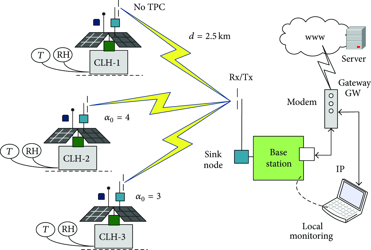
The original concept of the experimental marine environment WSN is a hierarchical approach composed of two tiers: a lower tier of 2.4 GHz low resource end-point (EP) wireless sensor node clusters and a 900 MHz upper tier of cluster-head (CLH) nodes with sensors onboard. For the CLH to communicate with both WSN tiers, it has two radios onboard: a short range 2.4 GHz coordinating transceiver (that communicates with the EP with a 300 m range) and a second 900 MHz radio for upper tier communications (capable of reaching up to 5 km). The CLH nodes create a 900 MHz wireless network with the sink node, which is connected to the WSN base station (BS) system.

In this project, the TRH TPC algorithm is meant to operate at the upper tier, between CLH and BS radios. The CLH systems are Arduino open hardware platforms [17], and the upper tier radio used in our test bed is the AC4490 digital transceiver [18, 19]. We choose the AC4490LR-1000 because it can transmit with any of 81 different power levels, with typical nonlinear power increments which range from 5 mW to 1000 mW, as shown in Figure 2. The AC4490 also comes with a set of on-the-fly configuration commands and instructions for acquiring its status.

Figure 2

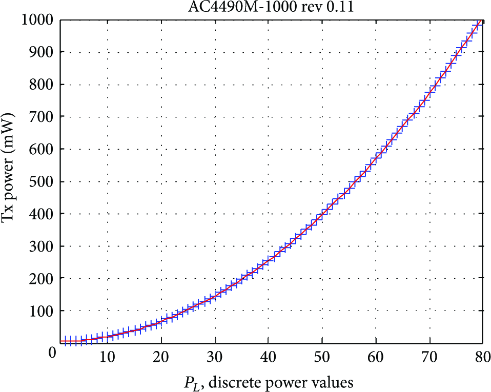
AC4490 nonlinear transmission power levels.

Likewise, when the AC4490 is receiving, it has a nonlinear Rx power reading as well. It can report valid RSSI levels in two ways: as an analog signal set at one of its output pins or as an 8-bit code word stored in an internal register called the “validated” RSSI (or VRSSI). This RSSI is also reported within the header of so-called Enhanced Receive Application Program Interface (API) frames. Equation (3) represents the formula for converting this raw RSSI value into a dBm interpretation:

$$\begin{array}{cc}& \mathrm{R}\mathrm{S}\mathrm{S}\mathrm{I}\mathrm{\hspace{0.17em}\hspace{0.17em}}\left(\mathrm{d}\mathrm{B}\mathrm{m}\right)=-\mathrm{46.9}\ast \frac{\mathrm{V}\mathrm{R}\mathrm{S}\mathrm{S}\mathrm{I}}{\mathrm{255}}-\mathrm{53.9}.\end{array}$$

(3)

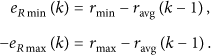
The minimum RSSI value the AC4490 can report is $-53.9$  dBm, as (3) shows when VRSSI is equal to 0. The discrete RSSI values that appear in a table that the manufacturer publishes in its users manual confirm this; from this table we generated the RSSI curve shown in Figure 3.

Figure 3

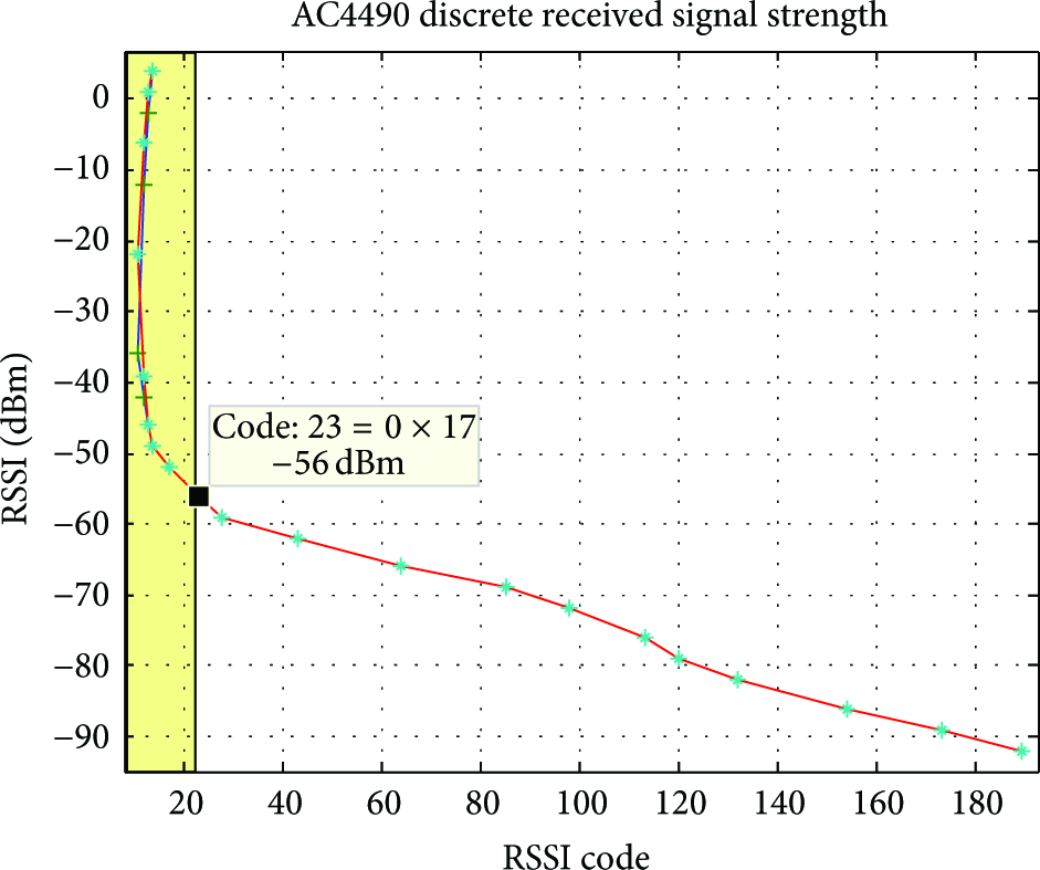
AC4490 RSSI curve, the shaded region is not valid.

2.2. Power Budget Analysis and Distance Emulation

Distance is an important issue because the CLH nodes at the upper tier create long range WSN. An RF power budget analysis is needed to determine the adequate Tx power to be able to reach various distances. The well-known path loss formula, expressed by (4), is typically used to determine the overall power attenuation an RF signal suffers due to operational frequency and distance traveled [20]:

$$\begin{array}{cc}& L_p\hspace{0.17em}\left(\mathrm{d}\mathrm{B}\right)=\mathrm{92.4}+\mathrm{20}\mathrm{l}\mathrm{o}\mathrm{g}\left(f_{\mathrm{G}\mathrm{H}\mathrm{z}}\right)+\mathrm{20}\mathrm{l}\mathrm{o}\mathrm{g}\left(d_{\mathrm{k}\mathrm{m}}\right).\end{array}$$

(4)

Another relevant equation is the effective irradiated power, ERP, expressed by

$$\begin{array}{cc}& \mathrm{E}\mathrm{R}\mathrm{P}\hspace{0.17em}\left(\mathrm{d}\mathrm{B}\right)=P_{\mathrm{T}\mathrm{x}}\hspace{0.17em}\left(\mathrm{d}\mathrm{B}\right)+G_{\mathrm{T}\mathrm{x}}\hspace{0.17em}\left(\mathrm{d}\mathrm{B}\right)-L_f\hspace{0.17em}\left(\mathrm{d}\mathrm{B}\right),\end{array}$$

(5)

where $P_{\mathrm{T}\mathrm{x}}\hspace{0.17em}(\mathrm{d}\mathrm{B})$ is the transmission power in $\mathrm{d}\mathrm{B}$ , $G_{\mathrm{T}\mathrm{x}}\hspace{0.17em}(\mathrm{d}\mathrm{B})$ is the transmitters antenna gain, and $L_f\hspace{0.17em}(\mathrm{d}\mathrm{B})$ is line feed loss (if any). Knowledge of $L_p$ and ERP can yield the received power, RSSI, by using

$$\begin{array}{cc}& \mathrm{R}\mathrm{S}\mathrm{S}\mathrm{I}\hspace{0.17em}\left(\mathrm{d}\mathrm{B}\right)=\mathrm{E}\mathrm{R}\mathrm{P}\hspace{0.17em}\left(\mathrm{d}\mathrm{B}\right)-L_p\hspace{0.17em}\left(\mathrm{d}\mathrm{B}\right).\end{array}$$

(6)

If the AC4490 transmitter is configured with its minimum power of 5 mW (or 7 dBm), using a simple 2 dBi antenna with negligible line feed loss, the minimum distance that the AC4490 receiver can be from the transmitter is 30.5 m. The latter also considers that the receiver's maximum RSSI power is equal to −53.9 dBm. This kind of radio has to be even farther apart if it uses higher Tx power levels. A method of emulating wireless distances between nodes for experimentation purposes is by attaching attenuators to their antennas and RF interface.

2.3. RF Noise, Data Acquisition, and Message Transfer

After many TRH-TPC deployment experiments, testing different parameter values, it became evident that to test the full range of TRH TPC parameter combinations it would take several weeks or months to finish. We decided to develop a simulation, described in the next subsection, using power budget equations and real data. With this aim, we reconfigured a CLH system modifying its code to do RF noise power sampling of its transceiver antenna interface along with simultaneous T and RH measurements. The AC4490 has two analog to digital converter (ADC) inputs, one of which is internally connected to the analog received signal strength output. To issue the AC4490 read RSSI command, the following hexadecimal values have to be put on its serial interface: $\mathrm{0}\mathrm{x}\mathrm{C}\mathrm{C},\hspace{0.17em}\mathrm{0}\mathrm{x}\mathrm{21},\hspace{0.17em}\mathrm{0}\mathrm{x}\mathrm{02}.$

The AC4490 responds with a 10-bit raw value at its serial output representing the instantaneous measured RF signal power. The actual power in mW is calculated with the following expression: $\mathrm{n}\mathrm{o}\mathrm{i}\mathrm{s}\mathrm{e}=\mathrm{53.9}-\mathrm{0.22}\ast \left(\mathrm{1023}-{\mathrm{r}\mathrm{a}\mathrm{w}}_{\mathrm{R}\mathrm{S}\mathrm{S}\mathrm{I}}\right).$

Figure 4 shows the experimental RF signal acquisition setup, where $P_L(n)$ is the transceiver discrete power level, ranging from 1 to $N_P=81$ . $\mathrm{P}\mathrm{R}\mathrm{R}(n)$ is the calculated packet received rate. $\mathrm{S}\mathrm{d}(n)$ are the sensor data samples (T, $\mathrm{R}\mathrm{H}$ , etc.). And $P_{\mathrm{T}\mathrm{x}}$ is the actual transmission power in mW, from 5 mW to 1000 mW, which directly depends on the configured $P_L(n)$ level. The CLH does data acquisition every sampling period, Ts, afterwards it constructs a message that sends to the BS. As soon as the BS receives this CLH message, it responds with an acknowledgement message containing the received message sequence number and the last RSSI value measured by its AC4490 sink node.

Figure 4

Experimental setup of CLH to BS communications.

Figures 5 and 6 show examples of CLH acquired T and RH data, and Figure 7 illustrates the resulting TRH gradient and its inverse. Moreover, Figure 8 represents an example of the measured RF signals acquired at the same time as T and RH, showing for the most part that the RF power levels follow the TRH gradient behavior.

Figure 5

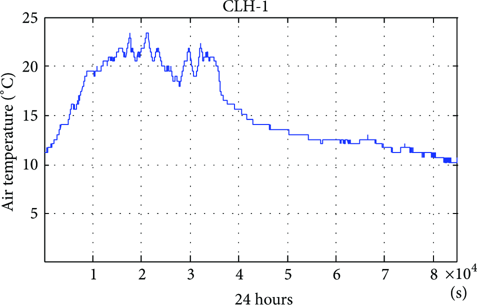
CLH-1 24-hour temperature readings.

Figure 6

CLH-1 24-hour relative humidity readings.

Figure 7

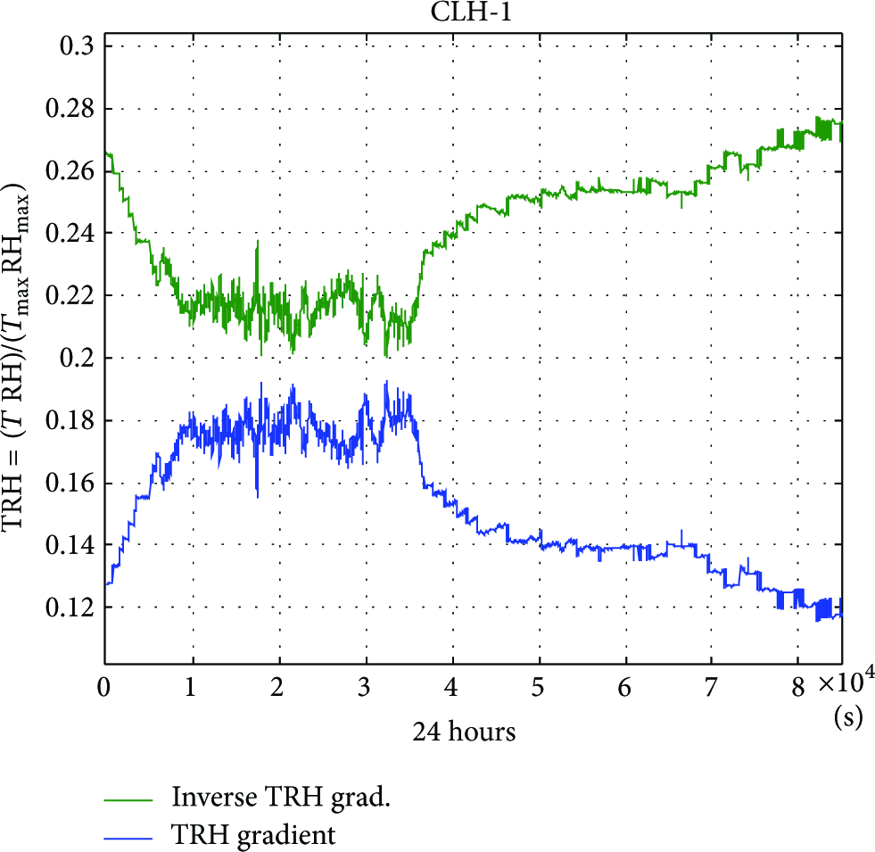
TRH gradient and its inverse.

Figure 8

AC4490 RF noise and interference signal measurements.

It is worth mentioning that the measured CLH data sent to the BS was relayed through an Internet connection towards a custom server, in charge of storing it in a database and within comma separated value (CSV) files. The system was left running exposed to real conditions for several days.

Figure 9 shows that, during this time, humidity measurements fell towards extreme dry conditions. And Figure 10 illustrates that the air temperature was 10°C higher during the day when RH dropped below 20% (Figure 9).

Figure 9

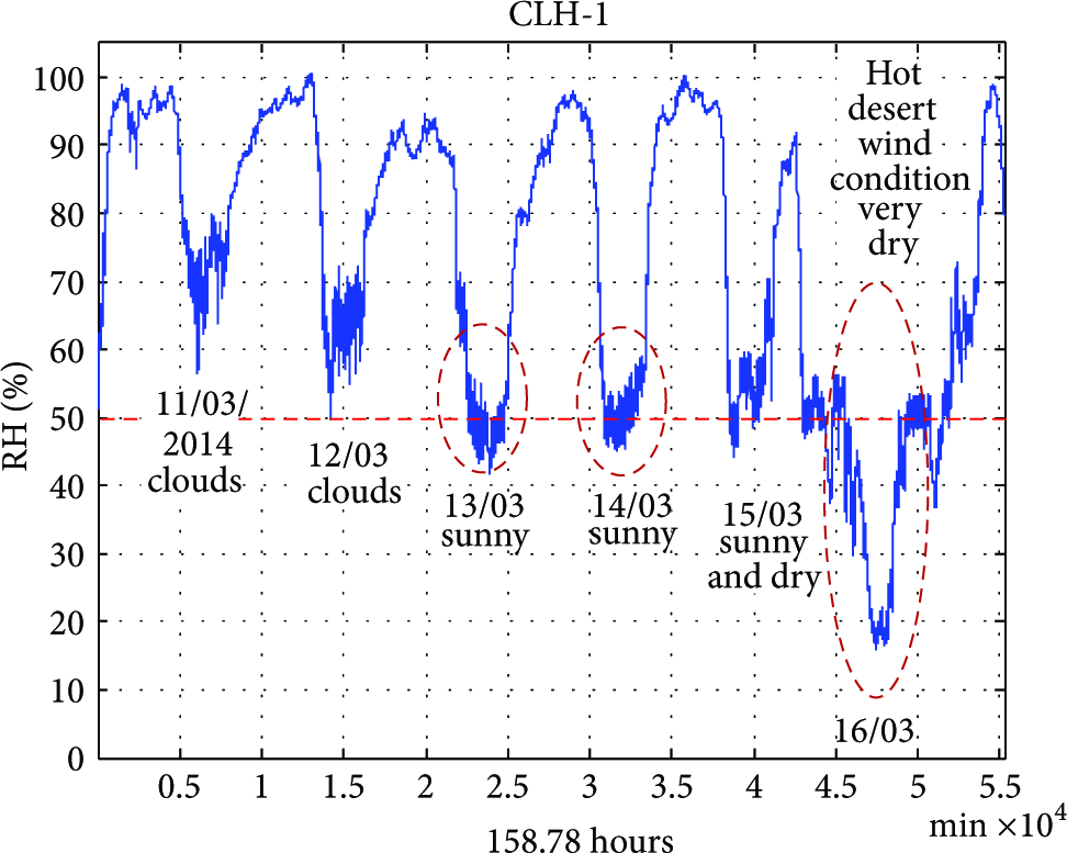
RH readings on a six-day experiment, with conditions below 50% RH.

Figure 10

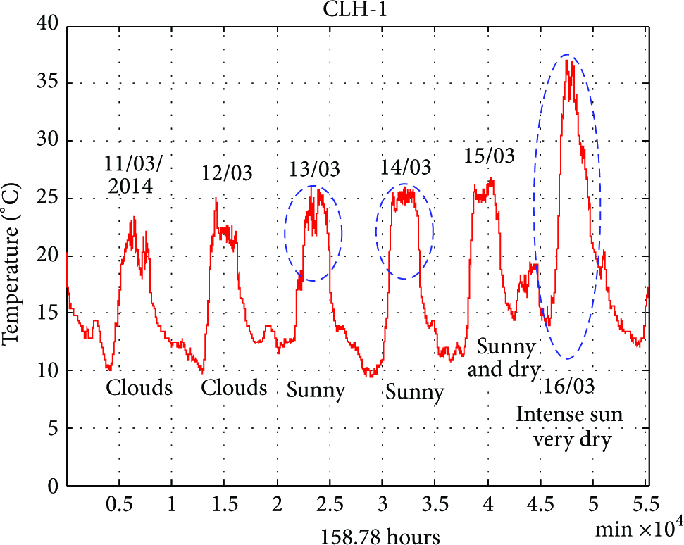
Temperature readings of a six-day experiment.

Figure 11 shows the resulting TRH gradient and Figure 12 illustrates the RF background noise. After comparing both figures with Figure 9, it is apparent that when RH is below 50% the TRH curve does not follow the RF background noise trend. Note that the TRH gradient, (1), can be useful as a TPC gain factor only if it follows the RF noise variations. The TRH distortion is remedied by adding an RH bias value to the TRH equation. After experimentation we found that the gradients’ useful behavior is guaranteed by adding 100% RH bias; the updated formula is expressed by

$$\begin{array}{cc}& \nabla \left(t\right)=\frac{T\left(t\right)\left(\mathrm{R}\mathrm{H}\left(t\right)+\mathrm{100}\right)}{T_{\mathrm{m}\mathrm{a}\mathrm{x}}{\mathrm{R}\mathrm{H}}_{\mathrm{m}\mathrm{a}\mathrm{x}}}.\end{array}$$

(7)

Figure 13 illustrates the biased TRH. Its values rise and fall in a similar manner as the noise behavior (Figure 12). Now this TRH gradient is more useful in the TPC gain factor equation expressed by (2).

Figure 11

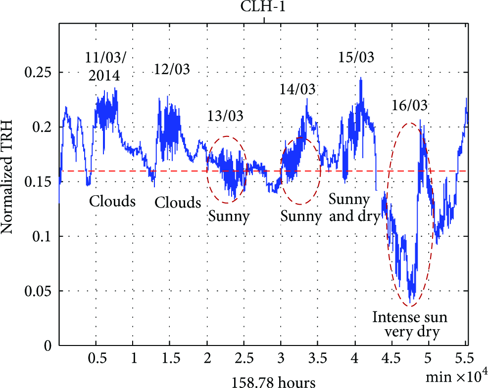
Plot of TRH during the six-day experiment.

Figure 12

RF noise and interference measurements on a six-day experiment.

Figure 13

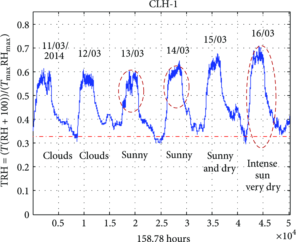
Biased TRH, which follows RF noise changes on a six-day experiment.

3. The Updated TRH-TPC Model

We made modifications to the original TRH-TPC scheme; it compared short average RSSI feedback against a single target set point, considered as the minimum RSSI threshold, $r_{\mathrm{m}\mathrm{i}\mathrm{n}}$ . Figure 14 shows our TRH TPC updated version that includes a maximum RSSI threshold, $r_{\mathrm{m}\mathrm{a}\mathrm{x}}$ .

Figure 14

TRH TPC system with RSSI hysteresis, bound by $r_{\mathrm{m}\mathrm{i}\mathrm{n}}$ and $r_{\mathrm{m}\mathrm{a}\mathrm{x}}$ .

In Figure 14, $G(z)$ represents the transmission power controller; Tx is the transmitter, $C(z)$ is the wireless channel, Rx is the receiver, and $r(z)$ is a short average RSSI value, measured at the receiver and fed back to the controller. Furthermore, $P_L(z)$ is the discrete power level established by $G(z)$ that sets the transmitters actual power, ${\mathrm{T}\mathrm{x}}_{\mathrm{P}\mathrm{m}\mathrm{W}(z)}$ . Meanwhile, ${\mathrm{R}\mathrm{x}}_{\mathrm{P}\mathrm{m}\mathrm{W}(z)}$ is the instantaneous RSSI measured by the receiver that is later sent to the CLH with a delay, $r(z-1)$ , which is compared to two thresholds, $r_{\mathrm{m}\mathrm{i}\mathrm{n}}$ and $r_{\mathrm{m}\mathrm{a}\mathrm{x}}$ , yielding two feedback errors $e_{R\mathrm{m}\mathrm{i}\mathrm{n}}\mathbf{\left(}z\mathbf{\right)}$ and ${-e}_{R\mathrm{m}\mathrm{a}\mathrm{x}}\mathbf{\left(}z\mathbf{\right)}$ expressed by

$$\begin{array}{cc}& e_{R\mathrm{m}\mathrm{i}\mathrm{n}}\left(k\right)=r_{\mathrm{m}\mathrm{i}\mathrm{n}}-r_{\mathrm{a}\mathrm{v}\mathrm{g}}\left(k-\mathrm{1}\right),\\ {-e}_{R\mathrm{m}\mathrm{a}\mathrm{x}}\left(k\right)=r_{\mathrm{m}\mathrm{a}\mathrm{x}}-r_{\mathrm{a}\mathrm{v}\mathrm{g}}\left(k-\mathrm{1}\right).\end{array}$$

(8)

The range between maximum and minimum thresholds is called a hysteresis zone in classical control system applications [21]. In this scheme, the hysteresis approach is used to avoid continual Tx power compensation around the minimum RSSI set point.

Within the $G(z)$ controller, the decision is made on which error to take into account for Tx power compensation. Algorithm 1 shows the corresponding pseudocode that describes actions that should be taken by the controller, where $P_L(k)$ is the discrete power level output by $G(z)$ , and the $P_L(k+1)$ is the updated power level that the transmitter will use during the next data transmission.

Algorithm 1: Updated TRH TPC algorithm with $$r_{\min }$$ and $$r_{\max }$$ thresholds.

C onstants: $$\mathtt{R}{\mathtt{H}}_{\mathtt{b}\mathtt{i}\mathtt{a}\mathtt{s}}$$ , TRHscale, $${\mathtt{N}}_{\mathtt{a}\mathtt{v}\mathtt{g}}$$ , a0

Input: $${\mathtt{T}}_{\mathtt{a}\mathtt{v}\mathtt{g}}$$ (k), $$\mathtt{R}{\mathtt{H}}_{\mathtt{a}\mathtt{v}\mathtt{g}}$$ (k),    $${\mathtt{r}}_{\mathtt{m}\mathtt{i}\mathtt{n}}$$ , $${\mathtt{r}}_{\mathtt{m}\mathtt{a}\mathtt{x}}$$ , r(k), $${\mathtt{r}}_{\mathtt{a}\mathtt{v}\mathtt{g}}$$ (k), $${\mathtt{P}}_{\mathtt{L}}$$ (k)

Ouput: $${\mathtt{P}}_{\mathtt{L}}$$ (k   +   1), $${\mathtt{P}}_{\mathtt{T}\mathtt{m}\mathtt{a}\mathtt{x}}$$ (k   +   1)

Initialization: k   =   0, jj   =   0

(1 )    loop:   TRH(k)   =   ( $${\mathtt{T}}_{\mathtt{a}\mathtt{v}\mathtt{g}}$$ ( k ) .   *   ( $$\mathtt{R}{\mathtt{H}}_{\mathtt{a}\mathtt{v}\mathtt{g}}$$ (k)   +   $$\mathtt{R}{\mathtt{H}}_{\mathtt{b}\mathtt{i}\mathtt{a}\mathtt{s}}$$ ) /TRHscale

(2 )    Gain:   TRH_delta(k)   =   1   −   exp( − a0.   *   TRH(k))

(3)  Average RSSI: $${\mathtt{r}}_{\mathtt{a}\mathtt{v}\mathtt{g}}$$ (k) = mean(r(k),    $${\mathtt{N}}_{\mathtt{A}\mathtt{V}\mathtt{G}}$$ )

(4 )    Compensation: jj ++   ==   $${\mathtt{N}}_{\mathtt{A}\mathtt{V}\mathtt{G}}$$ ?

(5 )                      $${\mathtt{r}}_{\mathtt{a}\mathtt{v}\mathtt{g}}$$ (k)   <   $${\mathtt{r}}_{\mathtt{m}\mathtt{i}\mathtt{n}}$$ ?

(6 )                              $${\mathtt{P}}_{\mathtt{L}}$$ (k   +   1)   =   $${\mathtt{P}}_{\mathtt{L}}$$ (k)   +   abs(TRH_delta(k).   *   ( $${\mathtt{r}}_{\mathtt{m}\mathtt{i}\mathtt{n}}$$   −   $${\mathtt{r}}_{\mathtt{a}\mathtt{v}\mathtt{g}}$$ (k)))

(7 )                      $${\mathtt{r}}_{\mathtt{a}\mathtt{v}\mathtt{g}}$$ (k)   >   $${\mathtt{r}}_{\mathtt{m}\mathtt{a}\mathtt{x}}$$ ?

(8 )                              $${\mathtt{P}}_{\mathtt{L}}$$ (k   +   1)   =   $${\mathtt{P}}_{\mathtt{L}}$$ (k)   +   abs(TRH_delta(k).   *   ( $${\mathtt{r}}_{\mathtt{a}\mathtt{v}\mathtt{g}}$$ (k)   −   $${\mathtt{r}}_{\mathtt{m}\mathtt{a}\mathtt{x}}$$ ))

(9 )                      else: $${\mathtt{P}}_{\mathtt{L}}$$ (k   +   1)   =   $${\mathtt{P}}_{\mathtt{L}}$$ (k)

(10 )                      jj   =   0

(11 )                  k++   //    next loop

There are two possible power adjustments because there are two error comparisons. Equation (9) is the updated power value if the delayed $r(k)$ is below the minimum threshold, and (10) is the next power value if the delayed $r(k)$ value is over the maximum threshold. Algorithm 1 shows the entire TPC process:

$$\begin{array}{cc}& P_L\left(k+\mathrm{1}\right)=P_L\left(k\right)+{\Delta }_N\left(k\right)e_{R\mathrm{m}\mathrm{i}\mathrm{n}}\left(k\right),\end{array}$$

(9)

$$\begin{array}{cc}& P_L\left(k+\mathrm{1}\right)=P_L\left(k\right)-{\Delta }_N\left(k\right)e_{R\mathrm{m}\mathrm{a}\mathrm{x}}\left(k\right).\end{array}$$

(10)

4. TRH TPC Simulation Using Real Data and Actual Nonlinear Tx Power Levels

We developed a simulation environment that uses the RF power budget equations described earlier; it also considers the AC4490 radio nonlinear Tx power levels. And to simulate a more realistic response, we loaded from CSV files real T, RH, and RF noise data. Algorithm 2 shows the simulation constant declarations and parameter initialization, along with real data vectors loaded from files. In this simulated environment, the TRH gradient and TPC gain factor calculation can be done a priori because we have T and RH beforehand.

Algorithm 2: TRH TPC algorithm initialization section.

S _Rx   =   − 100; % dBm AC4490 Rx sensitivity

Lp   =   − 92; % dB 1.2   Km path loss

AntGain   =   2; % dBi

$${\mathtt{r}}_{\mathtt{m}\mathtt{i}\mathtt{n}}$$   =   − 80; $${\mathtt{r}}_{\mathtt{m}\mathtt{a}\mathtt{x}}$$   =   −75;   % dBm , min and max RSSI thresholds

CLH_vals = load([my_data_path ‘RF915MHz_ACTUAL_noise.csv’]);

CLH_T   =   CLH_vals(:,   1);         % Acquire Temperature array

CLH_RH   =   CLH_vals(:,   2); % Acquire RH array

Nt   =   CLH_vals(:,   3);           % dBm RF noise sample array

L   =   length(Nt);               % Number of samples

TRH   =   (CLH_T.   *   (CLH_RH   +   100))/scale;   % 100% biased TRH Gradient

TRH_delta   =   1   −   exp( − alpha.   *   TRH); % TPC gain factor

PtxdB   =   10.   *   log10(pLEVEL); % dBw, pLEVEL is predefined

In Algorithm 3, the simulation does RSSI power calculations without TPC for future comparison purposes, with and without TPC, followed by RSSI short average estimations that will be used later during the actual compensation at the end of every averaging period. Moreover, in Algorithm 3, nonlinear AC4490 Tx power values in dB are loaded from a CSV file and converted to the dBm scale by subtracting 30 dB. And the power level vector $P_L(k)$ (set to the same RSSI vector dimension) is initialized with the preconfigured user selected mW power level converted to dBm.

Algorithm 3: RSSI calculation without TPC, RSSI short averaging, and loading of nonlinear AC4490 Tx power values.

R ssi   =   PtxdB   −   (S_Rx   +   Nt)   +   Lp   +   AntGain; % ref RSSI, without TPC

$${\mathtt{N}}_{\mathtt{a}\mathtt{v}\mathtt{g}}$$   =   10; % compensation window size

$${\mathtt{N}}_{\mathtt{b}\mathtt{l}\mathtt{o}\mathtt{c}\mathtt{k}}$$   =   10; % RSSI Averaging every Nblock samples

% Short average every RSSI $${\mathtt{N}}_{\mathtt{b}\mathtt{l}\mathtt{o}\mathtt{c}\mathtt{k}}$$ samples at a time

Rssi_avg   =   short_mean(Rssi,   $${\mathtt{N}}_{\mathtt{b}\mathtt{l}\mathtt{o}\mathtt{c}\mathtt{k}}$$ );

Tx_Pw = load(‘AC4490_Tx_Pl.csv’) − 30; % dBm

Pl   =   abs(ones(size(Rssi)).   *   10.   *   log10(TxPwmW); % dBm

Algorithm 4 shows our TRH TPC simulations main loop. It determines RSSI short average estimations every $N_{\mathrm{a}\mathrm{v}\mathrm{g}}$ sample, followed by its comparison with the minimum and maximum RSSI thresholds. If the RSSI average is below the $r_{\mathrm{m}\mathrm{i}\mathrm{n}}$ threshold then the compensation is positive, increasing power. Else, if the RSSI average is over the maximum $r_{\mathrm{m}\mathrm{a}\mathrm{x}}$ threshold, then the power compensation is negative, decreasing the radios power level. Else the Tx power is unchanged because the RSSI level is within the hysteresis zone.

Algorithm 4: TRH TPC main loop.

f or i   =   $${\mathtt{N}}_{\mathtt{a}\mathtt{v}\mathtt{g}}$$   :   L   −   1, % Main simulation loop

  % RSSI emulation using gain - loss equation affected by TRH TPC

  Rssi_adj(i)   =   Tx_Pw(floor(abs(Pl(i))))   −   (S_Rx   +   Nt(i))   +   Lp   +   AntGain; %dBm

  if(jj   ==   $${\mathtt{N}}_{\mathtt{a}\mathtt{v}\mathtt{g}}$$ ) % Do RSSI average after every $${\mathtt{N}}_{\mathtt{a}\mathtt{v}\mathtt{g}}$$ samples

      % Do a RSSI short average

      rssi_mean2(i)   =   mean(Rssi_adj((i   −   ( $${\mathtt{N}}_{\mathtt{a}\mathtt{v}\mathtt{g}}$$   −   1))   :   i));

      % Minimum Tx power threshold comparison

      if(rssi_mean2(i)   <   $${\mathtt{r}}_{\mathtt{m}\mathtt{i}\mathtt{n}}$$ ),

        % PL update   :   INCREASE Tx power

        Pl(i   +   1)   =   Pl(i)   +   abs(TRH_delta(i).*( $${\mathtt{r}}_{\mathtt{m}\mathtt{i}\mathtt{n}}$$   −   rssi_mean2(i)));

      else

        % Maximum Tx power threshold comparison

        if(rssi_mean2(i)   >   $${\mathtt{r}}_{\mathtt{m}\mathtt{a}\mathtt{x}}$$ ),

          % PL update   :   DECREASE Tx power

          Pl(i   +   1)   =   Pl(i)   −   abs(TRH_delta(i).*(rssi_mean2(i)   −   $${\mathtt{r}}_{\mathtt{m}\mathtt{a}\mathtt{x}}$$ ));

          if (Pl(i)   <   0), Pl(i   +   1)   =   0; end % ensures Pl not negative

        else

            Pl(i   +   1)   =   Pl(i); // power level unchanged

        end

      end

      jj   =   1; % re-initialize compensation window counter

  else

      jj   =   jj   +   1; % increment compensation counter

      rssi_mean2(i)   =   rssi_mean2(i   −   1);

    % keeps a constant average until it is time to update it

  end

end

Figure 15(a) shows the simulation environment input dialog, where the user chooses the key TRH TPC parameters, and Figure 15(b) shows plots of a two-day simulation example that uses previously acquired RF noise, T and RH data loaded from CSV files. The resulting RSSI levels without TPC, in dBm, are calculated adding the negative path loss and subtracting noise power from the constant transmission power.

Figure 15

Simulation environment example. (a) TRH TPC input dialog. (b) Set of plots that show real input noise, TRH gradient, and results of two days’ worth of samples.

After power compensation, the controlled RSSI (shown in green and averaged in red at the left hand lower corner of Figure 15) tends to stay within the minimum RSSI and maximum RSSI thresholds. In order to determine the algorithm performance, the minimum RSSI error is determined by counting the RSSI values that fall beneath the minimum RSSI threshold and dividing the result by the vectors total RSSI. Other useful plots in Figure 15 are the TRH biased gradient (upper right), the AC4490 discrete power levels (at the middle), and the radiated transmission power levels in mW (at the lower right corner).

5. TRH Parameter Optimization and Results

The TRH TPC algorithm operates using key parameters such as the alpha TRH gain coefficient, ${\alpha }_0$ , the controllers hysteresis zone, which ranges from $r_{\mathrm{m}\mathrm{i}\mathrm{n}}$ to $r_{\mathrm{m}\mathrm{a}\mathrm{x}}$ , and the selected time to do RSSI averaging, $T_{\mathrm{a}\mathrm{v}\mathrm{g}}$ . Here we did several experiments using our simulation environment changing these parameters to determine which values offered the best TPC results.

5.1. Alpha Coefficient Selection

The ${\alpha }_0$ argument affects the power gain step size; for example, Figure 16(a) illustrates a close-up view of the resulting RSSI of a TRH TPC simulation experiment with a low ${\alpha }_0=0.5$ and Figure 16(b) shows it with a high ${\alpha }_0=8$ . Comparison of both plots confirms that power compensation is slower with a low valued ${\alpha }_0$ than with a high alpha.

Figure 16

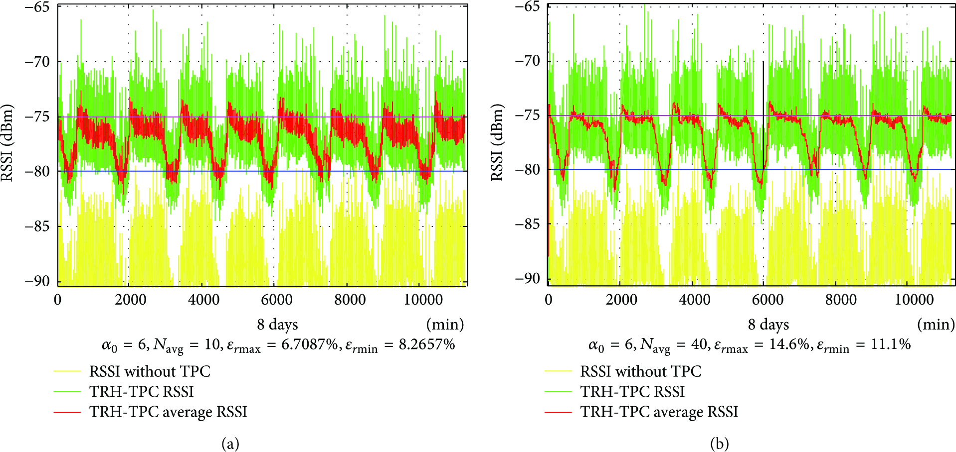
TRH TPC simulation RSSI plots, (a) using ${\alpha }_0$ = 0.5 and (b) using ${\alpha }_0$ = 8.

With ${\alpha }_0=8$ , the TPC response overshoots the maximum RSSI threshold by almost 5 dB. Another useful comparison is between the RSSI plots shown in Figures 17(a) and 17(b), which are zoomed out versions of Figures 16(a) and 16(b), respectively; it shows that compensation is faster with a high alpha because the RSSI level tends to go near the minimum RSSI threshold instead of staying mostly at the top near the maximum RSSI limit.

Figure 17

TRH TPC zoomed out simulation RSSI plots, (a) using ${\alpha }_0=0.5$ and (b) using ${\alpha }_0=8$ .

Originally we proposed ${\alpha }_0$ as a compressed gain factor to avoid unstable RSSI compensation. Also, it was previously found that, below 0.5, this alpha coefficient yields unitary power steps that cause a very slow convergence. At the upper limit, it was suggested that alpha should be equal to or less than 2 to avoid larger Tx power step sizes. Here we reevaluated the upper power limit because the RSSI variable changes faster in harsh sunlight interference than first observed.

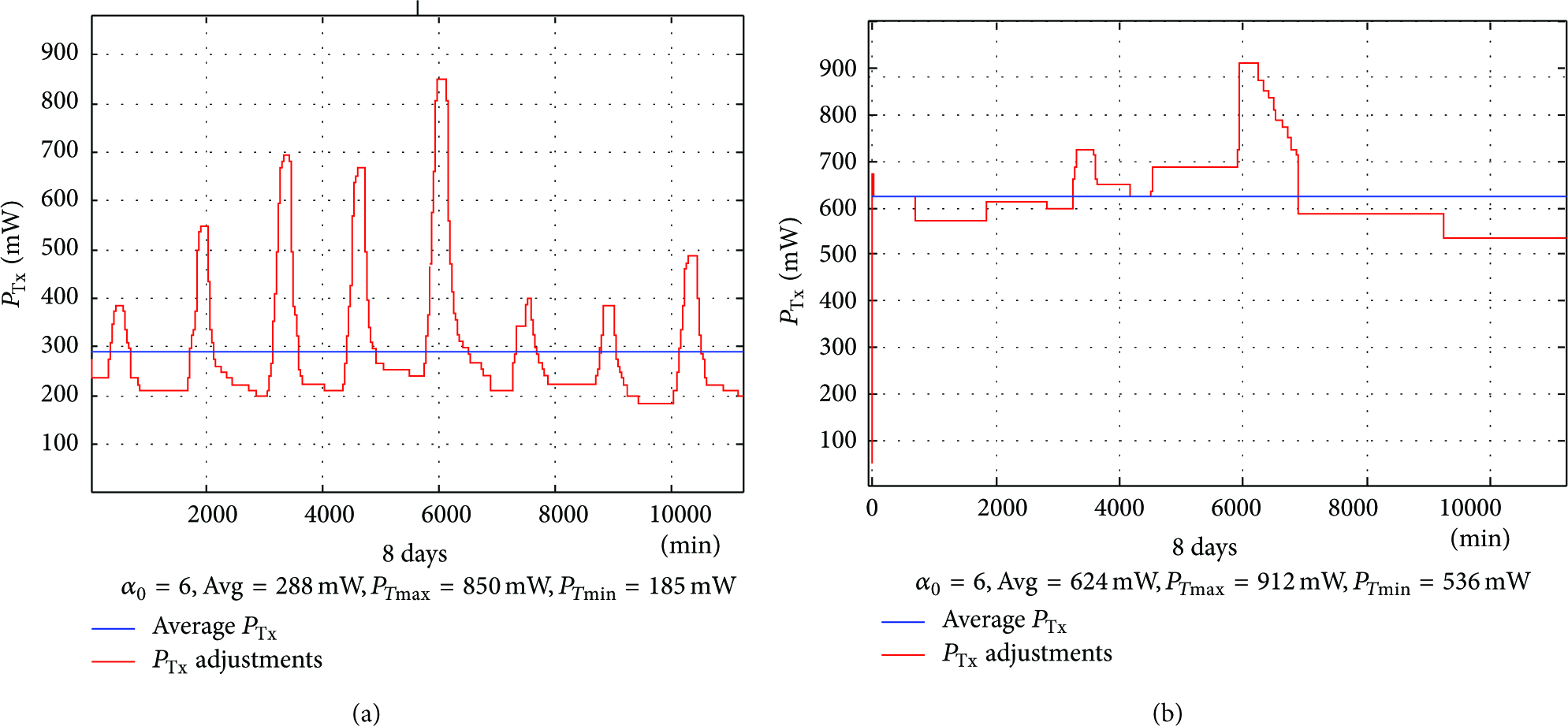
Figures 18(a) and 18(b) show plots of the resulting transmission power with ${\alpha }_0=0.5$ and ${\alpha }_0=8$ , respectively. Figure 18(b) illustrates that with ${\alpha }_0=8$ the initial compensation increases Tx power to more than 800 mW. In contrast, in Figure 18(a) with ${\alpha }_0=0.5$ the transmission power increase is less than 300 mW. The question remains on what ${\alpha }_0$ value can be considered an optimum limit. We decided to do several experiments with different ${\alpha }_0$ values, and through trial and error, good results were obtained with ${\alpha }_0$ less than or equal to 6.

Figure 18

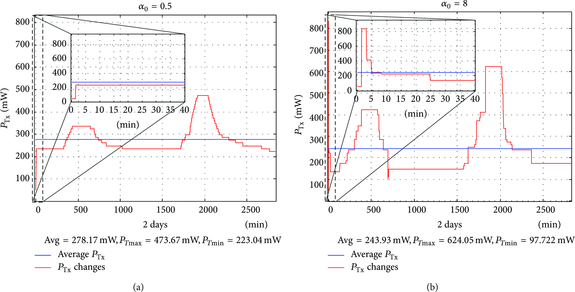
Transmission power plots in mW, (a) using ${\alpha }_0=0.5$ and (b) using ${\alpha }_0=8$ .

The TRH controllers’ aim is to regulate transmission power, so the RSSI levels rise or fall within the preestablished hysteresis zone. During this process, the received power may overshoot the $r_{\mathrm{m}\mathrm{a}\mathrm{x}}$ threshold, which represents an error that we call the maximum RSSI threshold error, ${\epsilon }_{\mathrm{m}\mathrm{a}\mathrm{x}}$ . Or on the contrary, the RSSI levels may go below the $r_{\mathrm{m}\mathrm{i}\mathrm{n}}$ causing a minimum RSSI threshold error, ${\epsilon }_{\mathrm{m}\mathrm{i}\mathrm{n}}$ . The latter is the least desirable error state for TPC because packet loss increases due to poor signal reception.

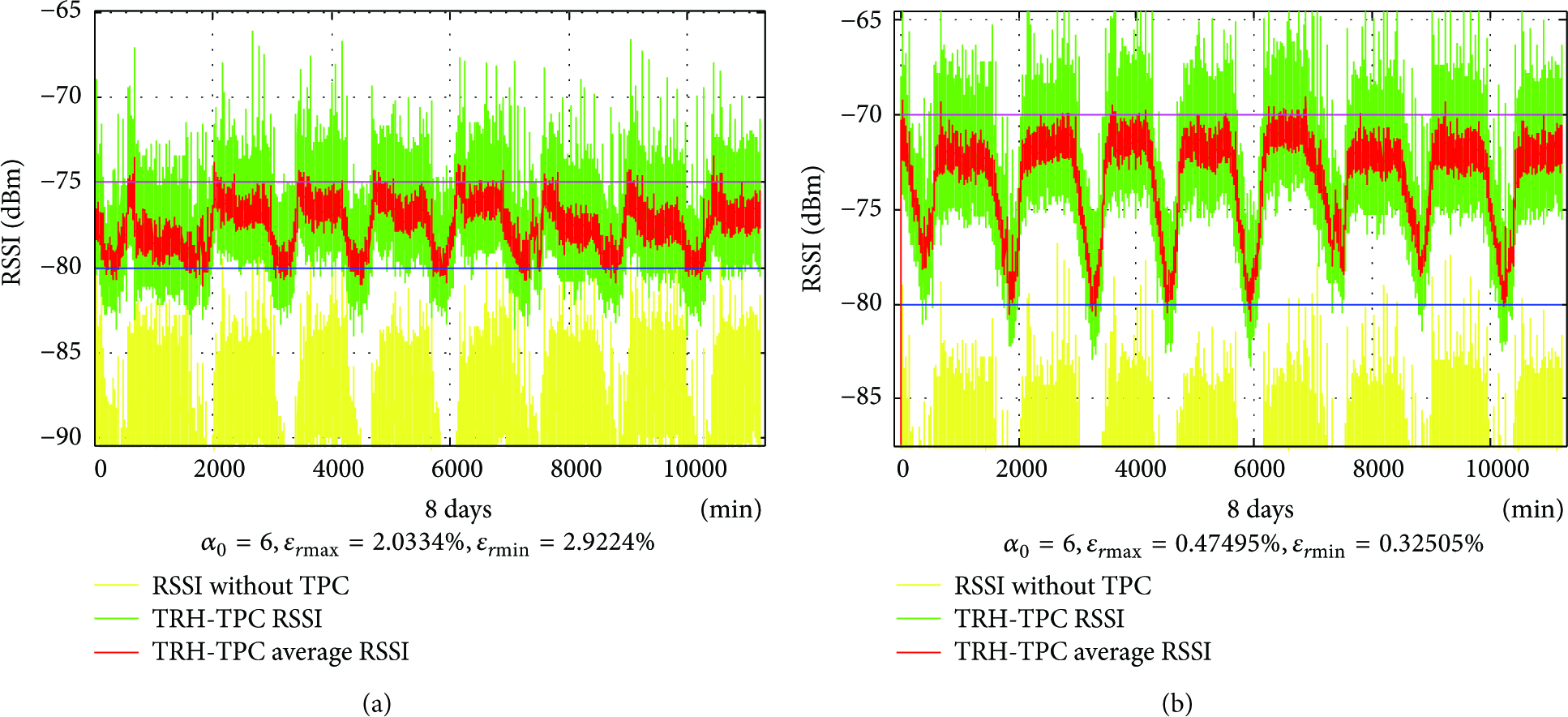
To determine the TRH algorithms performance with different ${\alpha }_0$ values, we included a variable that counts the RSSI short averages that go below the minimum RSSI threshold to obtain an estimate of the ${\epsilon }_{\mathrm{m}\mathrm{i}\mathrm{n}}$ metric. Likewise, to determine ${\epsilon }_{\mathrm{m}\mathrm{a}\mathrm{x}}$ a maximum RSSI error counter was included in the model and incremented when the RSSI short averages go over $r_{\mathrm{m}\mathrm{a}\mathrm{x}}$ . Many TRH experiments were done changing the alpha parameter and logging the amount of RSSI threshold errors. In Table 1 the estimated ${\epsilon }_{\mathrm{m}\mathrm{i}\mathrm{n}}$ and ${\epsilon }_{\mathrm{m}\mathrm{a}\mathrm{x}}$ values of an eight-day experiment are shown, along with the Tx power metrics corresponding to different alpha values.

Table 1

RSSI minimum error and Tx power metrics of an eight-day simulation with different $${\alpha }_{\mathit{0}}$$ .

${\alpha }_{\mathit{0}}$	${\epsilon }_{\mathtt{m}\mathtt{i}\mathtt{n}\hspace{0.17em}\text{\%}}$	${\epsilon }_{\mathtt{m}\mathtt{a}\mathtt{x}\hspace{0.17em}\text{\%}}$	$P_{\text{Txavg}}$ (mW)	$P_{\text{Txmin}}$ (mW)	$P_{\text{Txmax}}$ (mW)
0.5	13.1	14.3	294	210	612
1	11.3	10.6	292	198	674
2	9.9	8.2	291	198	724
4	8.5	7.0	289	185	800
6	8.3	6.7	288	185	840
8	8.2	6.6	294	185	870
10	8.1	6.6	300	185	900
12	8.1	6.6	310	185	915
14	8.1	6.6	310	185	920

In Table 2 twelve-day simulation results are presented, where estimated ${\epsilon }_{\mathrm{m}\mathrm{i}\mathrm{n}}$ and ${\epsilon }_{\mathrm{m}\mathrm{a}\mathrm{x}}$ values are shown, with corresponding transmission power characteristics. In Tables 1 and 2, after ${\alpha }_0=4$ the minimum errors did not change much. After several simulations using samples from different days, the Tx power behavior and RSSI values reflected similar results. Figures 19 and 20 illustrate plots of the RSSI threshold errors versus discrete alpha values of Tables 1 and 2, respectively. Figures 21 and 22 represent transmission power plots of eight- and twelve-day trials versus different alphas, respectively. In both plots, the average and minimum transmission power metrics are very similar for different ${\alpha }_0$ values.

Table 2

RSSI minimum error and Tx power metrics of a twelve-day simulation with different $${\alpha }_{\mathit{0}}$$ .

${\alpha }_{\mathit{0}}$	${\epsilon }_{\mathtt{m}\mathtt{i}\mathtt{n}\text{\hspace{0.17em}\%}}$	${\epsilon }_{\mathtt{m}\mathtt{a}\mathtt{x}\text{\hspace{0.17em}\%}}$	$P_{\text{Txavg}}$ (mW)	$P_{\text{Txmin}}$ (mW)	$P_{\text{Txmax}}$ (mW)
0.5	12.4	13.7	297	210	611
1	10.7	10.2	295	198	650
2	9.3	7.9	293	198	700
4	8.1	6.6	291	185	770
6	7.8	6.4	291	185	810
8	7.8	6.4	296	185	845
10	7.7	6.3	310	185	874
12	7.7	6.3	315	185	880
14	7.6	6.3	315	185	890

Figure 19

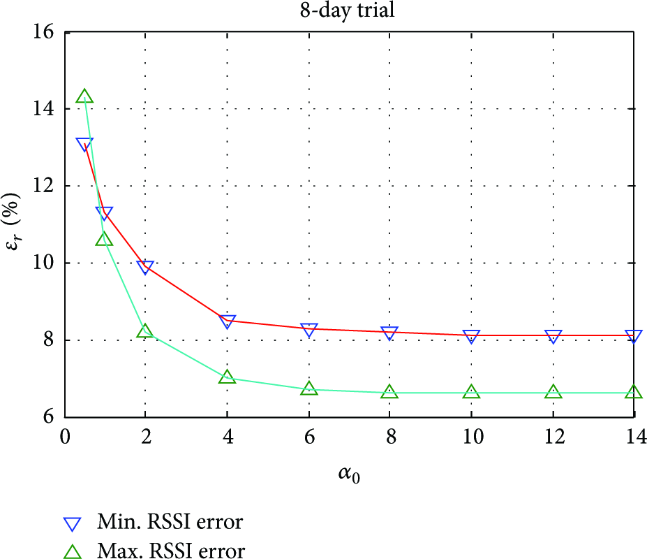
Eight-day trial RSSI threshold error versus ${\alpha }_0$ .

Figure 20

RSSI threshold error versus ${\alpha }_0$ , eight-day trial.

Figure 21

Transmission power versus ${\alpha }_0$ , eight-day trial.

Figure 22

Transmission power versus ${\alpha }_0$ , twelve-day trial.

After evaluating the TRH TPC performance with different ${\alpha }_0$ values, it is apparent that ${\alpha }_0$ can be much higher than previously assumed. Our updated ${\alpha }_0$ limit can be as high as 6 because the average transmitted power stays the same, and error performance does not improve much afterward. Moreover, after ${\alpha }_0=6$ the maximum transmission power increases unnecessarily.

5.2. RSSI Hysteresis Selection

Other relevant TRH TPC parameters are the minimum and maximum RSSI thresholds; the gap between them establishes an RSSI hysteresis zone, where the controllers power level output remains in a steady state response even when very small input variations occur [20]. Without this so-called hysteresis zone the controller would continually compensate the Tx power level with any slight RSSI change, which might make the scheme unstable by over stressing the radios reconfiguration process. Originally, the TRH controller set point was established to be exclusively the desired RSSI minimum value, $r_{\mathrm{m}\mathrm{i}\mathrm{n}}$ . Afterward, a maximum RSSI limit, $r_{\mathrm{m}\mathrm{a}\mathrm{x}}$ , was proposed and implemented in our deployments. Both set points determine the controllers RSSI hysteresis zone, or ${\mathrm{R}\mathrm{S}\mathrm{S}\mathrm{I}}_{\mathrm{H}\mathrm{y}\mathrm{s}}$ . Various simulation experiments were done changing the RSSI hysteresis width to determine the influence that threshold selection has on the RSSI behavior. Figures 23 and 24 show initial results with ${\alpha }_0=6$ using eight days’ worth of data testing two different hysteresis zones. Figure 23(a) illustrates the RSSI result and Figure 24(a) shows the transmission power involved in the process of a trial run with $r_{\mathrm{m}\mathrm{a}\mathrm{x}}=-75$  dBm. In contrast, Figure 23(b) is the RSSI plot and Figure 24(b) is the $P_{\mathrm{T}\mathrm{x}}$ plot with a maximum RSSI threshold of $-70$  dBm.

Figure 23

RSSI behavior with ${\alpha }_0$ = 6, (a) $r_{\mathrm{m}\mathrm{a}\mathrm{x}}=-75$  dBm and (b) $r_{\mathrm{m}\mathrm{a}\mathrm{x}}=-70$  dBm.

Figure 24

Transmission power behavior with ${\alpha }_0=6$ , (a) $r_{\mathrm{m}\mathrm{a}\mathrm{x}}=-75$  dBm, $P_{\mathrm{a}\mathrm{v}\mathrm{g}}$ = 288 mw; and (b) $r_{\mathrm{m}\mathrm{a}\mathrm{x}}=-70$  dBm, $P_{\mathrm{a}\mathrm{v}\mathrm{g}}$ = 613 mW.

After analyzing both Figures 24(a) and 24(b), several issues are apparent as follows.

• (1)

The average RSSI tends to stay near the maximum RSSI threshold.

(2)

The RSSI error metric is lower when the RSSI hysteresis is wider.

(3)

The transmission power behavior stops following the TRH gradient when the hysteresis gap is too wide.

(4)

As the hysteresis gap widens the average transmission power increases.

We did several experiments with different hysteresis gaps; all their results were very similar. We found that with a minimum RSSI of −80 dBm the controller operates well up until a maximum threshold RSSI of $-72$  dBm, which represents 3.28% of the entire RSSI span (this is considering a radio sensitivity of −100 dBm). Another way of stating the main observation is that the transmission power behavior mostly follows the maximum TRH values if a wide hysteresis zone is used $({\mathrm{R}\mathrm{S}\mathrm{S}\mathrm{I}}_{\mathrm{H}\mathrm{y}\mathrm{s}}>4\%)$ , which is an undesirable condition because the radio involved invests more transmission power than necessary to satisfy the minimum RSSI requirement.

5.3. Short Average Window Size and Compensation Cycle Issues

For the purpose of maintaining stability against sudden climate changes and deep fading, we proposed that the TRH TPC algorithm operates with short averaged values to be able to react accordingly. These are simple mean averages, which add values of a particular variable (be it T, RH, or RSSI) and divide them by the number of averaged samples. After every averaging operation, done every $N_{\mathrm{a}\mathrm{v}\mathrm{g}}$ samples, the TRH controller determines if power compensation is needed, according to previous Algorithm 4. By default, in our initial deployments, we did averaging every ten samples, $N_{\mathrm{a}\mathrm{v}\mathrm{g}}=10$ . We found that if we change the amount of averaged samples, widening the $N_{\mathrm{a}\mathrm{v}\mathrm{g}}$ window, the transmission power behavior also changes. Figure 25 shows two TRH controlled RSSI plots, with ${\alpha }_0=6$ . Figure 25(a) is the received signal strength using $N_{\mathrm{a}\mathrm{v}\mathrm{g}}=10$ sample window, and Figure 25(b) is the RSSI behavior averaging $N_{\mathrm{a}\mathrm{v}\mathrm{g}}=40$ samples.

Figure 25

RSSI behavior with ${\alpha }_0=6$ , (a) $N_{\mathrm{a}\mathrm{v}\mathrm{g}}=10$ and (b) $N_{\mathrm{a}\mathrm{v}\mathrm{g}}=40$ .

The RSSI curve of Figure 25(b) is much smoother than that of Figure 25(a). Nevertheless, in Figure 25(b) both RSSI threshold errors increased with more averaged samples. On the other hand, Figures 26(a) and 26(b) show the transmitted power plots in mW compensated every $N_{\mathrm{a}\mathrm{v}\mathrm{g}}=10$ and $N_{\mathrm{a}\mathrm{v}\mathrm{g}}=40$ samples, respectively. When we extended the averaging window from 10 samples to 40, the minimum transmitted power increased (from 185 mW to 248 mW), and the peak transmitted power decreased (from 850 mW to 624 mW). The overall effect of extending the averaging window caused an increase of the average power from 288 mW to 316 mW.

Figure 26

$P_{\mathrm{T}\mathrm{x}}$ behavior with ${\alpha }_0=6$ , (a) $N_{\mathrm{a}\mathrm{v}\mathrm{g}}=10$ and (b) $N_{\mathrm{a}\mathrm{v}\mathrm{g}}=40$ .

These simulations use data samples that are acquired every $\mathrm{T}\mathrm{s}=10$ seconds, with an averaging window of $N_{\mathrm{a}\mathrm{v}\mathrm{g}}=10$ samples, and the time between adjustments is $T_{\mathrm{a}\mathrm{v}\mathrm{g}}=100$ seconds (or 1.66 minutes). Likewise, with $N_{\mathrm{a}\mathrm{v}\mathrm{g}}=40$ samples power adjustments are made every 400 seconds (or 6.6 min.). The sensor sampling period depends on the application, but the time required to do TRH compensations depends on weather changes, which takes several minutes. Table 3 shows threshold error assessments and transmission power metrics obtained with different averaging windows. When widening the averaging window, two undesirable effects appear: (1) there is an unnecessary increase of the average transmitted power, representing useless power consumption, and (2) the amount of RSSI threshold errors increases notably.

Table 3

RSSI minimum error and Tx power metrics of a twelve-day simulation with different Navg sample window size, using $${\alpha }_{\mathit{0}}$$ = 6.

$N_{\text{avg}}$	$T_{\text{avg}}$ min $N_{\text{avg}}$ (Ts = 10 sec)/60	${\epsilon }_{\mathtt{m}\mathtt{i}\mathtt{n}\text{\hspace{0.17em}\%}}$	${\epsilon }_{\mathtt{m}\mathtt{a}\mathtt{x}\text{\hspace{0.17em}\%}}$	$P_{\text{Txavg}}$ (mW)	$P_{\text{Txmin}}$ (mW)	$P_{\text{Txmax}}$ (mW)
5	0.83	5.4	3.7	268	135	872
10	1.66	8.3	6.7	288	185	850
20	3.33	10.2	12.1	307	223	699
30	5.00	11.1	14.8	312	236	649
40	6.66	11.3	18.8	316	248	624
50	8.33	11.5	22.3	316	261	611
60	10.00	11.6	24.8	318	261	586
70	11.66	11.8	26.0	319	261	573
80	13.33	12.2	27.3	320	261	561
90	15.00	12.4	30.9	320	261	548
100	16.66	12.8	33.1	320	261	536
200	33.33	13.1	40.3	319	273	474
300	50.00	13.8	44.3	318	273	436

Figure 27 shows the plot corresponding to the RSSI errors listed in Table 3 against the averaging time window $T_{\mathrm{a}\mathrm{v}\mathrm{g}}$ . It is apparent that short averaging at less than 10 minutes yields better TPC results than otherwise. Also, it is notable that the most affected performance metric when increasing the time window is the maximum RSSI error: after 10 minutes it climbs over 25%. Figure 28 illustrates the transmission power invested with different $T_{\mathrm{a}\mathrm{v}\mathrm{g}}$ windows.

Figure 27

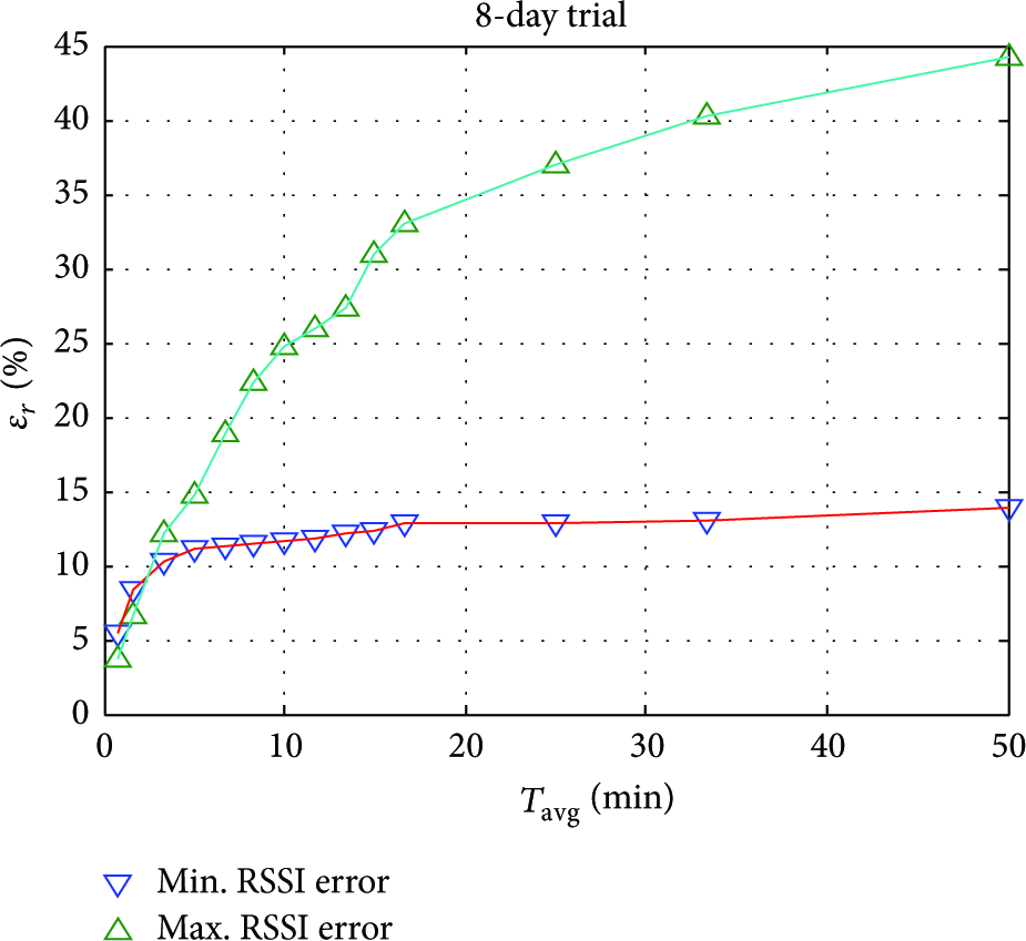
Minimum and maximum RSSI error versus $T_{\mathrm{a}\mathrm{v}\mathrm{g}}$ , ${\alpha }_0=6$ .

Figure 28

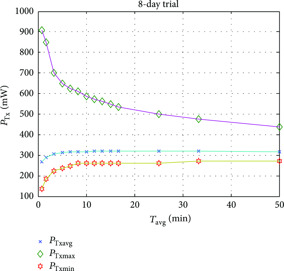
Transmission power metrics versus $T_{\mathrm{a}\mathrm{v}\mathrm{g}}$ , ${\alpha }_0=6$ .

Although in Figure 28 it might seem beneficial that with a wider $T_{\mathrm{a}\mathrm{v}\mathrm{g}}$ window less transmission power is consumed, the RSSI errors of Figure 27 discourage this idea.

5.4. Parameter Optimization Summary

In this research effort most of the general properties of the TRH TPC proposal from previous work are corroborated; one such statement is that the range of the alpha coefficient is the key of this scheme. With the development and use of our TRH simulation environment, we have new information that suggests that the upper alpha bound can be higher, and the separation between maximum and minimum RSSI threshold impacts on the average power consumption. Likewise, other issues for fine tuning the TRH TPC algorithm are now apparent, such as the need for an appropriate averaging window size, which in consequence sets the compensation cycle period for the TRH TPC operation.

Table 4 lists a brief summary of the updated criteria for the key TRH TPC parameters. Although some observations are tied to the particular test bed radio, the RSSI averaging period selection depends on how fast the wireless channel conditions change in real weather and not on the transceivers characteristics.

Table 4

Updated TRH TPC parameter summary.

TRH TPC parameter	Criteria	Description
$${\alpha }_{\mathit{0}}$$	2 < $${\alpha }_{\mathit{0}}$$ < 6	TRH TPC gain coefficient for a good convergence considering $${\epsilon }_{\mathtt{m}\mathtt{i}\mathtt{n}}$$ < 10% and $${\epsilon }_{\mathtt{m}\mathtt{a}\mathtt{x}}$$ < 10%.
$$\text{RSS}{\text{I}}_{\text{Hys}}$$	4% max.	Hysteresis percentage. RSSIHys = 100 * ( $$r_{\max }$$ − $$r_{\text{min}}$$ )/(full range RSSI) For minimal Tx power waste.
$$T_{\text{avg}}$$ = Ts $$N_{\text{avg}}$$	<10 minutes	RSSI averaging period = TRH TPC cycle Cycle sensitive to wireless channel conditions, which depends on the weather. In this test bed we considered Ts = 10 sec. and $$N_{\text{avg}}$$ < 60 samples.

By combining the criteria for all parameters, an optimum TRH TPC deployment can now be done. In order to finally corroborate these statements, we prepared and did a real experimental deployment, which is explained in the next final section.

6. Updated TRH TPC Real Deployment and Its Results

As explained in Section 2.1, in our initial WSN experimentation we worked with Arduino based systems with long range AC4490 radios, which we used again here to test the updated TRH TPC with the optimal parameters. The experimental setup consists of three ArduinoMega based CLH systems exposed to beach front weather conditions, as shown in the illustration of Figure 29. One CLH was set up to transmit at a fixed power level, and the other two were programmed with the real time TRH TPC algorithm. Software was developed using the controllers native C++ for embedded systems. Messages sent by the CLH towards the BS were answered by an acknowledgement message, ACK. During this feedback process, relevant metrics were communicated back to the CLH for its TRH TPC operations.

Figure 29

Experimental CLH setup for real testing of the optimal TRH TPC scheme.

All CLH systems were programmed to gather T and RH data and to maintain a counter of the ACK messages received back from the BS against the total sent after each transmission. It is worth noting that CLH-1 served as the reference system, it was not programmed with TPC, its radio was configured to transmit at a fixed 200 mW transmission power level, according to the minimum power needed to reach a 2.5 Km distance. Using wireless power budget calculations, the estimated RSSI level should be $-73$  dBm by excluding a fade margin. Meanwhile, CLH-2 and CLH-3 were programmed with the updated TRH TPC approach operating with ${\alpha }_0=4$ and ${\alpha }_0=3$ , respectively. Their radios were also configured at the same 200 mW, as the initial Tx power level.

In the case of CLH-1, Figure 30 shows its resulting RSSI levels; also Figure 31(a) is its temperature plot and Figure 31(b) is its RH measurements plot. Notice that the curves are reciprocal when comparing the RSSI with temperature, and the curves are proportional when comparing the RSSI with relative humidity. Also, Figure 32 shows the simultaneously measured RF signals at CLH-1 receiver input; notice that again its shape is reciprocal to the RSSI curve of Figure 30. The resulting CLH-1 PRR during this time is presented in Figure 33; its performance worsens during the day when the RSSI values are at their lowest levels.

Figure 30

RSSI values of the reference CLH-1 without TPC.

Figure 31

Reference CLH-1 without TPC (a) temperature and (b) relative humidity readings.

Figure 32

CLH-1 measured RF noise and/or interference.

Figure 33

CLH-1 packet received rate, operating without TPC and no retries reached 77.6%.

Meanwhile, Figures 34(a) and 34(b) show CLH-2 measured T and RH. Figures 35(a) and 35(b) illustrate CLH-2 calculated TRH gradient and measured RF noise floor at the time; notice that they have a similar shape. Moreover, Figure 36 shows CLH-2 transmission power adjustments, which follow the TRH gradient and noise floor changes.

Figure 34

Two-day CLH-2 (a) temperature and (b) relative humidity measurements.

Figure 35

Two-day CLH-2 (a) TRH gradient and (b) measured noise floor in dBm.

Figure 36

Two-day CLH-2 transmission power level adjustments.

The resulting two-day CLH-2 RSSI readings, measured at the BS and fed back to cluster-head, are plotted in Figure 37. The average CLH-2 RSSI (curve plotted in blue) was maintained within the maximum and minimum RSSI thresholds or hysteresis zone. And in Figure 38 a two-day CLH-2 PRR performance is illustrated obtaining a 96.94% average, which is 19% better than CLH-1 performance operating with no TPC.

Figure 37

Two-day CLH-2 controlled RSSI.

Figure 38

Two-day CLH-2 with TRH TPC packet received rate, with no Tx retries reaching a 96% PRR average.

On the other hand, Figures 39(a) and 39(b) show the temperature and relative humidity measured by the third CLH system. Also, Figures 40(a) and 40(b) illustrate the temperature TRH gradient calculated by CLH-3 and the measured RF noise floor at the same time. And Figure 41 represents CLH-3 plotted transmission power adjustments; notice that it follows the TRH gradient and RF noise floor changes.

Figure 39

Two-day CLH-3 (a) temperature and (b) relative humidity measurements.

Figure 40

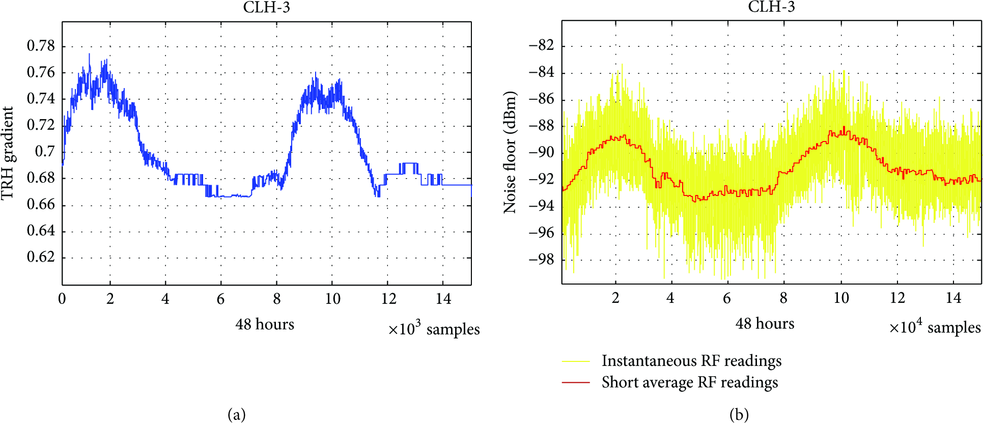
Two-day CLH-3 (a) TRH gradient and (b) measured noise floor in dBm.

Figure 41

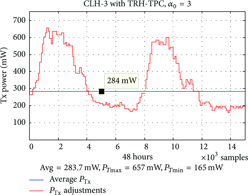
Two-day CLH-3 transmission power level adjustments.

The overall RSSI performance of CLH-3 to BS communications is shown in Figure 42, and its PRR performance is illustrated in Figure 43, which achieved a 95% PRR.

Figure 42

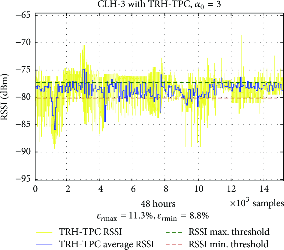
Two-day CLH-3 controlled RSSI.

Figure 43

The two-day packet received of CLH-3, with TRH TPC and no retries, reached a 95% average.

Table 5 presents a performance comparison summary between the different CLH system operations. Although CLH-1 reached the RSSI target a few times, transmitting at a fixed 200 mW level, only during the night it performed nearly as expected with an RSSI average 2 dB under the minimum threshold. Nevertheless, CLH-1 achieved a poor −88 dBm RSSI daytime average, which adversely affected its PRR reaching only a 77% packet delivery rate. In contrast, most of the time CLH-2 and CLH-3 maintained their RSSI averages within the minimum and maximum RSSI thresholds. This was reflected on their overall PRR performance, by delivering to BS over 95% of their transmitted packets.

Table 5

Two-day performance comparison of the updated TRH TPC.

CLH	RSSI avg. day/night dBm	PRR%	PL	$P_{\text{Tx}}$ mWnonlinearMax./min.	$P_{\text{Tx}}$ (dBm)	$P_{\text{Tx}}$ mWaverage
1  (no TPC)	−88/−82	77	36	208	20.1	208
2  ( $${\alpha }_{\mathit{0}}$$ = 4)	−79/−77	96	67 max 38 min	695/230	28.4/23.6	308
3  ( $${\alpha }_{\mathit{0}}$$ = 3)	−79/−77	95	65 max 32 min	657/165	28.2/22.2	284

For a medium term operational view, a seven-day CLH-2 experiment was done. Figure 44 shows the TRH gradient result and Figure 45 shows the measured RF noise floor during the time, which has a similar shape to the TRH gradient. Also, Figure 46 illustrates the Tx power adjustments done by the updated TRH TPC. From these results, CLH-2 consumed an overall 263 mW Tx power average and its level went down as low as 140 mW, which is better than the calculated 200 mW Tx power for a 2.5 Km distance from the intended receiver.

Figure 44

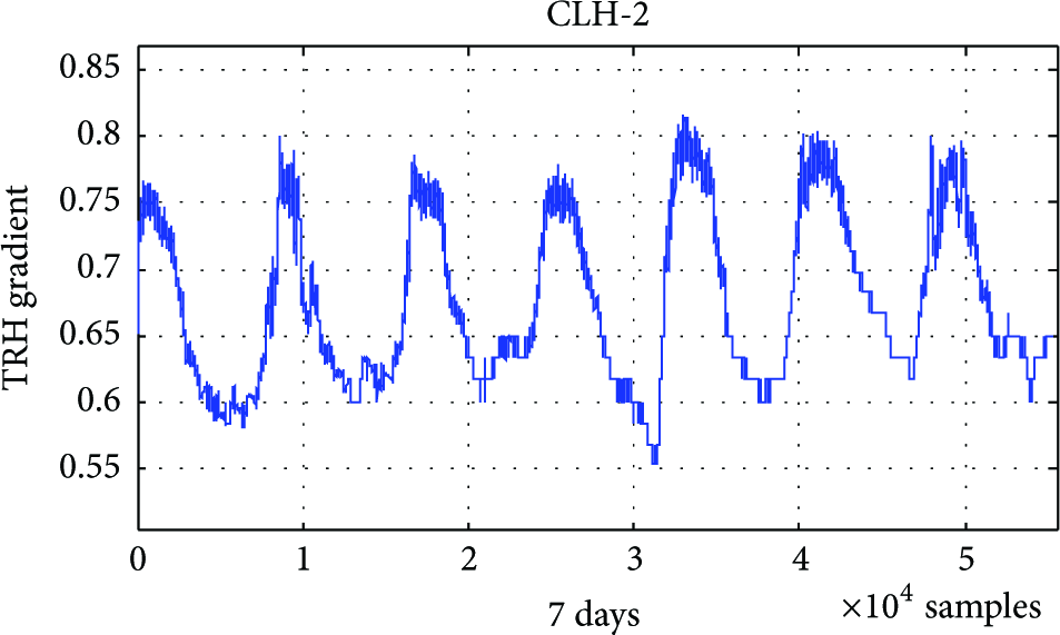
CLH-2 seven-day TRH gradient behavior.

Figure 45

CLH-2 seven-day noise floor measurements.

Figure 46

CLH-2 seven-day transmission power levels adjustments.

The overall RSSI and PRR performances of the seven-day CLH-2 experiment are shown in Figures 47 and 48, respectively. The measured RSSI levels were kept within the TRH TPC hysteresis zone. Likewise, the PRR performance was over 95%, which is a very good result considering that the radios had their Tx retry feature disabled. These results corroborate our initial TRH TPC experimental results previously mentioned to have been published in [15] and the optimal criterion results summarized in Section 5.4.

Figure 47

CLH-2 seven-day RSSI performance.

Figure 48

CLH-2 seven-day PRR performance.

These final real deployment results reflect the effectiveness of the simulation platform by obtaining similar real RSSI averages using the optimal parameter values, with a very good overall PRR of well over 90% without transmission retries.

7. Conclusions

In general, there is always a tradeoff between power consumption and best performance in wireless communications. It is also a fact that the rise in temperature negatively affects the resulting RSSI levels due to thermal noise at the receiver. Nevertheless, the discussion on the issue of air moisture and RF power attenuation is still ongoing. To be able to develop a practical model, atmospheric physicists have to do comprehensive studies with a well thought out methodology that takes into account a wireless engineering perspective. The published experimental approximations are often equations that are impractical for real-time TPC systems. Here, we did not pretend to model the exact way temperature and humidity hinder communications. We only observed the relative day-night RSSI power loss behavior and compared it to changes in T and RH, which yielded the TRH gradient. We then proposed a TRH TPC scheme with a minimum RSSI objective and a maximum RSSI threshold, which represents a nonlinear approach with RSSI feedback that depends on T and RH for Tx power compensation with a stabilizing power level hysteresis zone.

In particular, this paper presents experimental results that reflect the conditions under which this novel T and RH based TPC technique works best. The main contributions are that (1) we determined an updated the practical range for the proposed alpha gain coefficient, which should be between 2 and 6; (2) we updated the control model by including a Tx power level hysteresis zone, where the power level output variable maintains a steady state even when channel conditions change slightly, and determined a maximum hysteresis width of 4% of the total Tx power range; and (3) we found that the optimal power averaging time window should be equal to or less than 10 minutes for outdoor applications. Through this body of work, we have corroborated the usefulness of the TRH TPC proposal, and we established the basis for fine tuning the parameters involved in the power compensation process for long range communications. The development and extensive use of our TRH TPC simulation environment that uses real input values (RF noise, T and RH), accelerated our research effort. We then put to the test the TPC TRH algorithm running on real wireless systems operating in harsh conditions, and its result followed the expected behavior observed during simulations. Future work involves experimentation with real wireless sensor platforms so as to consolidate our TRH TPC concept for a marine habitat monitoring design space.