Lifetime Optimization Algorithm with Mobile Sink Nodes for Wireless Sensor Networks Based on Location Information

Abstract

In order to overcome the energy hole problem in some wireless sensor networks (WSNs), lifetime optimization algorithm with mobile sink nodes for wireless sensor networks (LOA_MSN) is proposed. In LOA_MSN, hybrid positioning algorithm of satellite positioning and RSSI positioning is proposed to save energy. Based on location information, movement path constraints, flow constraint, energy consumption constraint, link transmission constraint, and other constraints are analyzed. Network optimization model is established and decomposed into movement path selection model and lifetime optimization model with known grid movement paths. Finally, the two models are solved by distributed method. Sink nodes gather data of sensor nodes along the calculated paths. Sensor nodes select father nodes and transmit data to corresponding sink node according to local information. Simulation results show that LOA_MSN makes full use of node energy to prolong network lifetime. LOA_MSN with multiple sink nodes also reduces node energy consumption and data gathering latency. Under certain conditions, it outperforms MCP, subgradient algorithm, EASR, and GRAND.

1. Introduction

In most cases all sensor nodes of WSNs are battery-powered and located in the unattended or harsh environment. Battery replacement is difficult or even impossible for battery replacement. Once node's energy exhausts, the node is disabled. It will affect the network operation and even split the network to shorten network lifetime [1, 2]. Therefore, in WSNs, network lifetime is the important indicator of network performance. The algorithms of WSNs should save the energy and maximize the network lifetime.

Some scholars research on lifetime optimization algorithm with fixed nodes for WSNs and have got some accomplishments. For example, [3] proposes an ant colony optimization approach for maximizing the lifetime of heterogeneous wireless sensor networks. In the algorithm, cover constraint, collection constraint, and routing constraint are considered. The objective function is established and ant colony optimization is used to obtain the lifetime optimal scheme. Reference [4] constructs optimal clustering architecture and designs energy-aware cluster-head rotation and routing protocol to maximize network lifetime. Reference [5] proposes two methods to optimize the lifetime of chain-based protocols using integer linear programming (ILP) formulations. In those algorithms, it is inevitably to cause unbalanced distribution of node energy consumption and energy hole problem. The problem can be overcome by sink nodes’ movement. All nodes have the opportunity to transmit data near sink nodes and have the same lifetime.

References [6–9] research on the network lifetime maximization problem, establish the network lifetime optimization models with mobile sink node, use optimization algorithms to solve the models, and obtain optimal scheme. Reference [10] theoretically discusses the relationship between network lifetime and maximum throughout in the large scale WSNs. However, all references [6–10] assume that the movement path of sink node is already known and do not consider how to determine the anchors or movement path of sink node. Reference [11] searches guide agent nodes and intermediate guide nodes, analyzes the TSP (traveling salesman problem), determines movement path with node cooperation, and proposes data gathering algorithm which optimizes data transmission latency and energy. However, the algorithm does not consider network lifetime. Reference [12] divides network into several grids, and proposes a grid-based clustering algorithm. Reference [13] proposes range constrained clustering (RCC). RCC divides nodes into several clusters. Sink node stays at the cluster centers to gather data. The Concorde TSP solver is used to calculate the shortest movement path of sink node through some cluster centers. References [11–13] determine the locations of mobile sink node. However, they do not consider the data gathering when sink node is moving. Whether the algorithms can obtain optimal solution still needs theoretical analysis. Reference [14] proposes energy-aware sink relocation (EASR) algorithm for mobile sinks. EASR uses maximum capacity path (MCP) protocol for routing, starts to move when two relocation conditions are met, and finds the next moving location which has the greatest weight value. But compared with network lifetime, the relocation conditions are met after a long time. The protocol is not good at prolonging network lifetime.

Therefore, lifetime optimization algorithm with mobile sink nodes for wireless sensor networks based on location information (LOA_MSN) is proposed. In LOA_MSN, energy-saving positioning algorithm of nodes is proposed and the monitoring area is divided into several grids of the same size. Sink node can move into each grid center to gather data. The movement path constraints, flow constraint, energy consumption constraint, link transmission constraint, and other constraints are analyzed. The network optimization model is established. Then, the network optimization model is decomposed into movement path selection model and network lifetime optimization model with known movement paths. The movement path selection model is solved in sink nodes by distributed clustering method and graph theory method. Mobile gathering and static gathering are considered and the network lifetime optimization model is approximately solved by distributed graph theory method. Compared with MCP, subgradient algorithm, EASR and GRAND (for grid random scheme), LOA_MSN uses the node energy as much as possible to prolong the network lifetime.

The remaining parts of paper are organized as follows. In Section 2, the energy-saving positioning algorithm of nodes is proposed. In Section 3, the algorithm assumption and lifetime optimization model with mobile sink nodes are proposed. In Section 4, the distributed solution of model is proposed. In Section 5, the simulation results are presented. In Section 6, the paper is concluded.

2. Energy-Saving Positioning Algorithm

At present, mostly outdoor positioning uses satellite positioning module such as GPS or Beidou. But the work current of those modules is up to tens of milliamp. In the energy limited WSNs, they have great energy consumption. RSSI (received signal strength indication) positioning algorithm obtains the signal energy through link signal and has low energy consumption. Therefore, the hybrid positioning algorithm of satellite positioning and RSSI positioning is proposed to save energy. Assume that each node is equipped with Beidou or GPS positioning module. After network starts, sensor nodes and sink nodes periodically start the positioning module to obtain their longitude and latitude values. Due to the locations of sensor nodes being fixed, the time interval of sensor nodes is much longer than that of sink nodes. When there are more than 3 sensor nodes in the 1-hop communication range of sink node, the sink node shuts down the satellite positioning module for some time and uses RSSI positioning algorithm based on latest satellite positioning coordinates. The implementation of hybrid positioning algorithm is as follows.

Sink nodes transmit positioning query packets to nearby sensor nodes. Sensor nodes in the 1-hop communication range of sink nodes transmit their location information which is obtained by satellite positioning module, node address, and other information back to the corresponding sink node. Sink nodes receive a packet and obtain the RSSI value of link signal. If there are historical RSSI data of the same link, Kalman filtering is used to reduce errors and improve positioning accuracy [15]. Based on processed RSSI values, link distance $d_i$ from sensor node i to sink node is evaluated as follows:

$$\begin{array}{cc}& d_i=\mathrm{1}{\mathrm{0}}^{-({\text{RSSI}}_i+A)/\left(\mathrm{10}\text{Loss}\right)},\end{array}$$

(1)

where ${\text{RSSI}}_i$ represents the processed signal strength value of link from sensor node i to sink node. A represents the received signal strength value when the distance between transmitter and receiver is 1 m. Its value range is 30–50. Loss represents path loss exponent, namely, attenuation rate of signal energy. Its value range is 1–8. Through data communication, sink nodes obtain the location information of multiple sensor nodes and distances to those senor nodes and use multipoint positioning algorithm to calculate its coordinates with the following formula:

$$\begin{array}{l}\mathrm{2}\left[\begin{array}{c}{x}_{N_s}-x_{\mathrm{1}}\\ ⋮\\ x_{N_s}-x_{N_s-\mathrm{1}}\end{array}\right.\left.\begin{array}{c}{y}_{N_s}-y_{\mathrm{1}}\\ ⋮\\ y_{N_s}-y_{N_s-\mathrm{1}}\end{array}\right]\left[\begin{array}{c}{x}_s^R\\ y_s^R\end{array}\right]\\ \hspace{1em}=\left[\begin{array}{c}\left(d_{\mathrm{1}}^{\mathrm{2}}-d_{N_s}^{\mathrm{2}}\right)-\left(x_{\mathrm{1}}^{\mathrm{2}}-x_{N_s}^{\mathrm{2}}\right)-\left(y_{\mathrm{1}}^{\mathrm{2}}-y_{N_s}^{\mathrm{2}}\right)\\ ⋮\\ \left(d_{N_s-\mathrm{1}}^{\mathrm{2}}-d_{N_s}^{\mathrm{2}}\right)-\left(x_{N_s-\mathrm{1}}^{\mathrm{2}}-x_{N_s}^{\mathrm{2}}\right)-\left(y_{N_s-\mathrm{1}}^{\mathrm{2}}-y_{N_s}^{\mathrm{2}}\right)\end{array}\right],\end{array}$$

(2)

where $(x_i,y_i)$ , $i\in (\mathrm{1,2},\dots ,N_s)$ , represents the x- and y-coordinates of sensor node i which are the neighbor node of sink node. $(x_s^R,y_s^R)$ represents the x- and y-coordinates of sink node with RSSI positioning algorithm. $N_s$ represents the number of neighbor sensor nodes around the sink node.

Sink node records the elapsed time after the satellite positioning module is shut down. According to the satellite positioning coordinates $(x_s^w,y_s^w)$ , RSSI positioning coordinates $(x_s^R,y_s^R)$ , the elapsed time $t_L$ , and the movement speed u of sink node, the intersection point between the circle whose center is $(x_s^w,y_s^w)$ and radius is $t_L*u$ and the line from $(x_s^R,y_s^R)$ to $(x_s^w,y_s^w)$ is the current coordinates $(x_s^{},y_s^{})$ of sink node

$$\begin{array}{cc}& x_s=\frac{t_{L}u}{\sqrt{{\left(y_s^w-y_s^R\right)}^{\mathrm{2}}/{\left(x_s^w-x_s^R\right)}^{\mathrm{2}}+\mathrm{1}}}+x_s^w,\\ y_s=\frac{t_{L}u(y_s^w-y_s^R)}{(x_s^w-x_s^R)\sqrt{{\left(y_s^w-y_s^R\right)}^{\mathrm{2}}/{\left(x_s^w-x_s^R\right)}^{\mathrm{2}}+\mathrm{1}}}+y_s^w.\end{array}$$

(3)

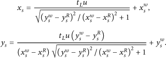
By the energy-saving positioning algorithm, nodes calculate their x- and y-coordinates with periodic start of satellite positioning module. It reduces the energy consumption of nodes.

3. Establishment of Optimization Model

In the paper, only 2D (two-dimensional) WSNs are considered and all nodes know their own location coordinates. The algorithm assumption is as follows. The locations of sensor nodes are fixed. Sink nodes can move to any grid center based on location information. All sensor nodes continuously transmit their sensing data to sink nodes. All sensor nodes have the same performance (such as sensing rate, maximum communication radius, initial energy, and energy consumption parameter). Energy of all nodes is limited, but energy of sink nodes can be renewable.

3.1. Constraints

3.1.1. Movement Path Constraints

Many references consider that sink node stays at one node location, gathers data, and takes its responsibilities to sense. It basically limits the mobile location selection of sink node and does not consider other locations where sensor node never distributes. Therefore, their algorithms obtain local optimal solutions. As is shown in Table 1, monitoring area is divided into several grids of the same size and each grid is numbered. The sink node can stay at each grid center to gather data. The method enlarges the selection range of sojourn locations for sink nodes.

Table 1

Grids in the monitoring area.

1	2	⋯	$$n-\mathit{1}$$	n
$$n+\mathit{1}$$	$$n+\mathit{2}$$	⋯	$$\mathit{2}n-\mathit{1}$$	$$\mathit{2}n$$
⋮	⋮	⋮	⋮	⋮
( $$n-\mathit{2}$$ ) $$n+\mathit{1}$$	( $$n-\mathit{2}$$ ) $$n+\mathit{2}$$	⋯	$$n^{\mathit{2}}-n-\mathit{1}$$	$$n^{\mathit{2}}-n$$
( $$n-\mathit{1}$$ ) $$n+\mathit{1}$$	( $$n-\mathit{1}$$ ) $$n+\mathit{2}$$	⋯	$$n^{\mathit{2}}-\mathit{1}$$	$$n^{\mathit{2}}$$

The mth sink node starts at initial location and finally moves back to the initial location. The initial location constraints of mth sink node are as follows:

$$\begin{array}{cc}& {\displaystyle \sum }_{w\in Gd}{p}_{s,w}^m=\mathrm{1},\hspace{1em}\forall m,\\ {\displaystyle \sum }_{w\in Gd}{p}_{w,s}^m=\mathrm{1},\hspace{1em}\forall m,\end{array}$$

(4)

where s represents ${\text{grid}}_s$ and initial location of mth sink node, ${\text{grid}}_v$ represents the center of grid v, and Gd represents the set of all grid centers. $p_{v,w}^m$ is the state indicator, which represents whether $L({\text{grid}}_v,{\text{grid}}_w)$ appears in the movement path of mth sink node. $L({\text{grid}}_v,{\text{grid}}_w)$ represents the directed line segment from ${\text{grid}}_v$ to ${\text{grid}}_w$ . $p_{v,w}^m=\mathrm{1}$ represents $L({\text{grid}}_v,{\text{grid}}_w)$ is in the movement path of mth sink node. As is shown in Table 1, the grids ( $1,n,(n-1)n+1$ , $n^2$ ) have only 2 neighbor grids and 2 line segments to neighbor grids. The other boundary grids have 3 neighbor grids. Others (such as $n+1$ , $2n-1$ ) have 4 neighbor grids.

Because each sink node cyclically moves along the path, the sum of state indicators which represent from ${\text{grid}}_v$ to all its neighbor grid centers is equal to the sum of state indicators which represent from all neighbor grid centers to ${\text{grid}}_v$ . The state indicator balance constraint is

$$\begin{array}{l}{\displaystyle \sum }_{w\in Gd,L({\text{grid}}_v,{\text{grid}}_w)\in Ld}{p}_{v,w}^m\\ \hspace{1em}={\displaystyle \sum }_{w\in Gd,L\left({\text{grid}}_v,{\text{grid}}_w\right)\in Ld}{p}_{w,v}^m,\hspace{1em}\forall v\in Gd,\hspace{0.17em}\forall m,\end{array}$$

(5)

where Ld represents the set of all possible line segments.

To avoid two mutually movable grids and eliminate the subtours, the state indicator limitation constraint is

$$\begin{array}{cc}& p_{v,w}^m+p_{w,v}^m\le \mathrm{1},\hspace{1em}\forall w,v\in Gd,\hspace{0.17em}\forall m.\end{array}$$

(6)

3.1.2. Flow Constraint

The transmission data are composed of the sensing data and received data from neighbor nodes. The flow constraint is

$$\begin{array}{cc}& {\displaystyle \sum }_{j\in N\left(i\right)}{f}_{ij}^m=S_i+{\displaystyle \sum }_{j\in N\left(i\right)}{f}_{ji}^m,\hspace{1em}\forall i\in V_m,\hspace{0.17em}\forall m,\end{array}$$

(7)

where $S_i$ represents the data sensing rate of node i and $f_{ij}^m$ represents the data transmission rate from node i to node j when the data of node i aggregate to mth sink node. $V_m$ represents a nonempty set of sensor nodes which are in the gathering range of mth sink node. $N(i)$ represents the neighbor node set of node i in $V_m$ .

3.1.3. Energy Consumption Constraint

During the gathering time 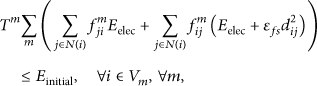$T_{}^m$ of mth sink node, the energy consumption of receiving data from neighbor nodes is $T_{}^m{\sum }_m^{}{\sum }_{j\in N(i)}^{}{f}_{ji}^m{E}_{\text{elec}}$ , where $E_{\text{elec}}$ represents electric energy consumption of receiving or transmitting unit data. The energy consumption of transmitting data is $T_{}^m{\sum }_m^{}{\sum }_{j\in N(i)}^{}{f}_{ij}^m(E_{\text{elec}}+{\epsilon }_{fs}{d}_{ij}^{\mathrm{2}})$ , where ${\epsilon }_{fs}$ represents electronic energy consumption of amplifying unit signal. The total energy consumption is not larger than initial energy. The energy consumption constraint is

$$\begin{array}{l}{T}_{}^m{\displaystyle \sum }_m\left({\displaystyle \sum }_{j\in N\left(i\right)}{f}_{ji}^m{E}_{\text{elec}}+{\displaystyle \sum }_{j\in N\left(i\right)}{f}_{ij}^m\left(E_{\text{elec}}+{\epsilon }_{fs}{d}_{ij}^{\mathrm{2}}\right)\right)\\ \hspace{0.5em}\hspace{1em}\le E_{\text{initial}},\hspace{1em}\forall i\in V_m,\hspace{0.17em}\forall m,\end{array}$$

(8)

where $E_{\text{initial}}$ represents the initial energy of sensor nodes.

3.1.4. Link Transmission Constraint

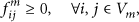
Because link bandwidth resource is limited, the total amount of link transmission data is limited. Then the link transmission constraint is

$$\begin{array}{cc}& f_{ij}^m+f_{ji}^m\le R_{\max },\hspace{1em}L\left(i,j\right)\in L_m,\hspace{1em}j>i,\hspace{0.17em}\forall m,\end{array}$$

(9)

where $R_{\max }$ represents the maximum transmission rates of nodes, $L(i,j)$ represents the link from node i to node j, and $L_m$ represents the set of all wireless links in all sensor nodes of $V_m$ .

3.2. Network Optimization Model

When network starts, sink node leaves from initial location to next grid center and finally moves back to initial location. The data gatherings of sink node are mobile gathering and static gathering. The mobile gathering of sink node is that, during its movement, sink node dynamically gathers data. The static gathering of sink node is that it stays at some grid centers for some sojourn time and statically gathers data.

The total time of mth sink node movement is

$$\begin{array}{cc}& T_{}^m={\displaystyle \sum }_n\hspace{0.17em}{\displaystyle \sum }_p{t}_p^{n,m}+\frac{{\sum }_n^{}{\sum }_{v\in Gd}^{}{\sum }_{w\in Gd}^{}{d}_{vw}{p}_{v,w}^m}{u},\end{array}$$

(10)

where $T_{}^m$ represents total time of mth sink node movement. $t_p^{n,m}$ represents the sojourn time in which mth sink node stays at $\text{gri}{\text{d}}_p$ in its nth movement. $d_{vw}$ represents the distance between $\text{gri}{\text{d}}_v$ and ${\text{grid}}_w$ . u represents the movement speed of sink nodes.

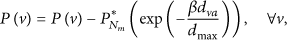
If there is one sink node in the network, formula (10) represents the network lifetime 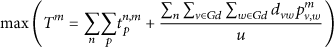$T_{\text{net}}$ . If there are several sink nodes, sink nodes broadcast their location information before gathering data. Sensor nodes select the nearest sink node to transmit data. Then the network is divided into multiple clusters. The network lifetime $T_{\text{net}}$ is defined as the average value of all $T^m$ ; namely, $T_{\text{net}}={\sum }_m^{}{T}^m/M$ , where M represents the number of sink nodes. The optimization problem of multiple sink nodes is transformed into multiple optimization problems of single sink node. The lifetime optimization model of mth sink node is

$$\begin{array}{cc}& \max \left(T_{}^m={\displaystyle \sum }_n{\displaystyle \sum }_p{t}_p^{n,m}+\frac{{\sum }_n^{}{\sum }_{v\in Gd}^{}{\sum }_{w\in Gd}^{}{d}_{vw}{p}_{v,w}^m}{u}\right)\end{array}$$

(11a)

s.t. Constraints (4)–(6)

$$\begin{array}{c}{\displaystyle \sum }_{j\in N\left(i\right)}{f}_{ij}^m=S_i+{\displaystyle \sum }_{j\in N\left(i\right)}{f}_{ji}^m,\hspace{1em}\forall i\in V_m,\end{array}$$

(11b)

$$\begin{array}{l}{T}_{}^m{\displaystyle \sum }_m\left({\displaystyle \sum }_{j\in N\left(i\right)}{f}_{ji}^m{E}_{\text{elec}}+{\displaystyle \sum }_{j\in N\left(i\right)}{f}_{ij}^m\left(E_{\text{elec}}+{\epsilon }_{fs}{d}_{ij}^{\mathrm{2}}\right)\right)\\ \hspace{1em}\hspace{1em}\le E_{\text{initial}},\hspace{1em}\forall i\in V_m,\end{array}$$

(11c)

$$\begin{array}{c}{f}_{ij}^m+f_{ji}^m\le R_{\max },\hspace{1em}L\left(i,j\right)\in L_m,\hspace{1em}j>i,\end{array}$$

(11d)

$$\begin{array}{c}{t}_p^{n,m}\ge \mathrm{0},\hspace{1em}\forall v,m,n,\end{array}$$

(11e)

$$\begin{array}{c}{f}_{ij}^m\ge \mathrm{0},\hspace{1em}\forall i,j\in V_m,\end{array}$$

(11f)

$$\begin{array}{c}{p}_{v,w}^m\in \left\{\mathrm{0,1}\right\},\hspace{1em}\forall v,w\in Gd.\end{array}$$

(11g)

4. Solution Method

Network optimization model (11a) considers movement path selection of sink node and data routing. The model has too many parameters and its solution is complicated. In the model, movement path constraints mainly limit ${\sum }_n^{}{\sum }_{v\in Gd}^{}{\sum }_{w\in Gd}^{}{d}_{vw}{p}_{v,w}^m/u$ in target function. It means finding a relatively optimal path. The flow constraint, energy consumption constraint, and link transmission constraint mainly limit ${\sum }_n^{}{\sum }_p^{}{t}_p^{n,m}$ in target function. It means searching optimal lifetime and routing solution. In order to reduce solving complication, the network optimization model (11a) is divided into movement path selection model and lifetime optimization model with known movement paths.

4.1. Movement Path Selection Model

The movement path constraints are too loose for path selection. It does not consider the node density and node energy. It needs a lot of time to calculate the solution of the model. Therefore, the path selection of sink nodes needs to consider the node location information and energy and determines some anchors for sink nodes. The anchors are some locations around where node density is high and residual energy of nodes is large. The clustering methods can be used to determine the anchors at which sink nodes stay to gather data of sensor nodes. In the paper, modified subtractive clustering algorithm is used to calculate the anchors [16]. The number and the set of anchors which mth sink node needs to stay at are obtained. The implementation steps of mth sink node are as follows.

Step 1.

The number of anchors is $N_m=1$ . The potential value of each grid is initialized as follows:

$$\begin{array}{ll}P\left(v\right)& =x_{\mathrm{1}}{\displaystyle \sum }_{j\in N\left(v\right)}^{}\exp \left(-\frac{{\alpha }_{\mathrm{1}}{d}_{vj}}{d_{\max }}\right)\\ & +x_{\mathrm{2}}{\displaystyle \sum }_{j\in N\left(v\right)}^{}\exp \left(-\frac{{\alpha }_{\mathrm{2}}{E}_{\text{initial}}}{\mathrm{Re}\left(j\right)}\right),\end{array}$$

(12)

where $P(v)$ represents potential value of grid _v . $d_{vj}$ represents the distance from sensor node j to grid center grid _v . $N(v)$ represents the set of sensor nodes from which the distance to grid center is no longer than maximum communication distance $d_{\max }$ . $\mathrm{Re}(j)$ represents the residual energy of node j. ${\alpha }_{\mathrm{1}}$ represents distance potential factor. ${\alpha }_{\mathrm{2}}$ represents residual energy potential factor. $x_1$ represents distance weight factor. $x_2$ represents residual energy weight factor, and $x_1+x_2=1$ .

Step 2.

The grid of maximum potential value is found. Its grid center as anchor point is selected. $P_{N_m}^{*}$ represents its potential value.

Step 3.

The grid center is aggregation point. Potential values of the grids are subtracted by formula

$$\begin{array}{cc}& P\left(v\right)=P\left(v\right)-P_{N_m}^{*}\left(\exp \left(-\frac{\beta d_{va}}{d_{\max }}\right)\right),\hspace{1em}\forall v,\end{array}$$

(13)

where β represents attenuation factor. $d_{va}$ represents the distance from grid center grid _v to the aggregation point.

Step 4.

If the following inequality holds, end the algorithm; otherwise $N_m=N_m+1$ and go to Step 2:

$$\begin{array}{cc}& \underset{v}{\max }\hspace{0.17em}P\left(v\right)\le \epsilon P_{\mathrm{1}}^{*},\end{array}$$

(14)

where ε represents judgment factor.

Network environment is complicated. The mobile gathering efficiency of sink nodes is far lower than static gathering efficiency. Therefore the movement time of sink nodes is as short as possible. Movement distance of mth sink node in one data gathering period is ${\sum }_{v\in Gd}^{}{\sum }_{w\in Gd}^{}(d_{vw}{p}_{v,w}^m)/u$ . Size of each grid is the same. Therefore, the movement path selection model of all sink nodes can be represented as follows when anchors are determined:

$$\begin{array}{cc}& \hspace{0.17em}\min {\displaystyle \sum }_{v\in Gd}\hspace{0.17em}{\displaystyle \sum }_{w\in Gd}{p}_{v,w}^m\end{array}$$

(15a)

$$\begin{array}{c}\hspace{0.17em}\text{s}.\text{t}.\text{:}{\displaystyle \sum }_{w\in Gd}{p}_{v,w}^m=\mathrm{1}\hspace{1em}{\displaystyle \sum }_{w\in Gd}{p}_{w,v}^m=\mathrm{1},\hspace{1em}\forall v\in \left\{P^m,s\right\},\hspace{0.17em}\forall m,\\ \text{Constraints}\mathrm{\hspace{0.17em}\hspace{0.17em}}\text{(4)–(6), (11g),}\end{array}$$

(15b)

where $P^m$ represents the set of anchors which is obtained by the modified subtractive clustering algorithm.

Model (15a) shows that the movement path selection of sink nodes is essentially TSP problem. It can be solved by genetic method, graph theory, and other methods. Because the number of anchors is not large, nearest neighbor interpolation algorithm is used to find the approximate solution of shortest path [17]. The implementation steps of mth sink node are as follows.

Step 1.

The location of sink node is initialized and $i=0$ . The anchor $v_0$ is the starting point. The initial closed path is $v_0\hspace{0.17em}\hspace{0.17em}{v}_0$ .

Step 2.

In $\{P^m,s\}-\{v_0,v_1,\dots ,v_i\}$ , anchor $v_{i+1}$ is found which has the nearest distance to any anchor in $\{v_0,v_1,\dots ,v_i\}$ set.

Step 3.

The anchor $v_{i+1}$ is inserted into the closed path $v_0\hspace{0.17em}\hspace{0.17em}{v}_1\cdots v_i\hspace{0.17em}\hspace{0.17em}{v}_0$ . The paths $v_0\hspace{0.17em}\hspace{0.17em}{v}_{i+1}\hspace{0.17em}\hspace{0.17em}{v}_1\cdots v_i\hspace{0.17em}\hspace{0.17em}{v}_0$ and $v_0\hspace{0.17em}\hspace{0.17em}{v}_1\hspace{0.17em}\hspace{0.17em}{v}_{i+1}\cdots v_i\hspace{0.17em}\hspace{0.17em}{v}_0,\dots ,v_0\hspace{0.17em}\hspace{0.17em}{v}_1\cdots \hspace{0.17em}{v}_i\hspace{0.17em}\hspace{0.17em}{v}_{i+1}\hspace{0.17em}\hspace{0.17em}{v}_0$ are obtained. The shortest path is selected as the new shortest closed path.

Step 4.

If $i<(N_m+1)$ , then go to Step 2; otherwise obtain the approximate solution, and go to Step 5.

Step 5.

According to the approximate solution, namely the obtained close path, sink node moves along the directed line segment from one anchor to its next anchor periodically. If sink node stays at the end anchor in the path, it moves back to initial anchor. Then all possible grids which sink node passes through are founded in turn. The selected anchors and grid centers constitute the solution of movement path selection model (15a). The grid centers that the sink node stays at, namely, the grid movement paths of sink nodes, are obtained.

4.2. Lifetime Optimization Model

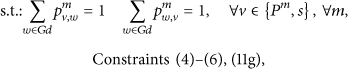
When the grid movement paths of sink nodes are determined, according to the definition of network lifetime, network lifetime optimization model can be transformed to the models of single sink node. Their target is to obtain the lifetime $T^m$ and node transmission rates $f_{ij}^m$

$$\begin{array}{l}\max \hspace{1em}\hspace{0.5em}{T}^m={\displaystyle \sum }_n\hspace{0.17em}{\displaystyle \sum }_p{t}_p^{n,m}+\frac{{\sum }_n^{}{\sum }_{v\in Gd}^{}{\sum }_{w\in Gd}^{}{d}_{vw}{p}_{v,w}^m}{u}\\ \end{array}$$

(16)

s.t.: Constraints (11b)–(11f).

The mobile gathering process of sink nodes is considered as sink nodes stay at the grid centers which are in their grid movement paths for some sojourn time to gather data. Therefore, the mobile gathering problem is converted into discrete multiple static gathering problems whose sojourn time is $d_{vw}/u$ . The lifetime is composed of sojourn times for which sink nodes stay at the anchors and passing grid centers.

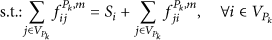
Therefore, the model is simplified. The lifetime optimization problem is transformed to several lifetime optimization models in which sink node stays at different grid centers. When mth sink node stays at location $P_k$ , the lifetime optimization model is

$$\begin{array}{c}\hspace{0.17em}\max \hspace{0.17em}{T}_v\end{array}$$

(17a)

$$\begin{array}{c}\hspace{0.17em}\text{s}.\text{t}.\text{:}{\displaystyle \sum }_{j\in V_{P_k}}{f}_{ij}^{P_k,m}=S_i+{\displaystyle \sum }_{j\in V_{P_k}}{f}_{ji}^{P_k,m},\hspace{1em}\forall i\in V_{P_k}\end{array}$$

(17b)

$$\begin{array}{c}\hspace{0.17em}\left({\displaystyle \sum }_{j\in V_{P_k}}{f}_{ji}^{P_k,m}{E}_{\text{elec}}+{\displaystyle \sum }_{j\in V_{P_k}}{f}_{ij}^{P_k,m}\left(E_{\text{elec}}+{\epsilon }_{fs}{d}_{ij}^{\mathrm{2}}\right)\right)\\ \hspace{1em}\hspace{1em}\le \frac{E_{\text{initial}}}{T_v},\hspace{1em}\forall i\in V_{P_k}\end{array}$$

(17c)

$$\begin{array}{c}\hspace{0.17em}\hspace{1em}{f}_{ij}^{P_k,m}+f_{ji}^{P_k,m}\le R_{\max },\hspace{1em}L(i,j)\in L_m,\hspace{1em}j>i\end{array}$$

(17d)

$$\begin{array}{c}\hspace{0.17em}\hspace{1em}\hspace{1em}\hspace{1em}{f}_{ji}^{P_k,m}\ge \mathrm{0},\hspace{1em}\forall i,\hspace{0.17em}j\in V_{P_k},\end{array}$$

(17e)

where $T_v$ represents the network lifetime when mth sink node stays at location $P_k$ , $f_{ij}^{P_k,m}$ represents the data transmission rate from node i to node j when the data of node i aggregate to mth sink node and mth sink node stays at location $P_k$ . $V_{P_k}$ represents the set of sensor nodes whose data aggregate to mth sink node. If node j is not the neighbor node of node i, $f_{ij}^{P_k,m}=\mathrm{0}$ . The lifetime optimization model (17a) can be solved by optimization methods such as distributed subgradient method [18] and approximately solved by distributed graph methods [19].

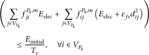
In the paper, in order to reduce the time complexity of the algorithm, the model (17a) is approximately solved by the distributed asynchronous Bellman-Ford algorithm. Namely, when sink node starts to gather data, it transmits data query packets from time to time. Then, the implementation steps of sensor node i are as follows.

Step 1.

If sensor node i receives the routing information packet of its sink node, the address and shortest path weight $D_s(t)=\mathrm{0}$ of sink node are added to the information table of neighbor nodes. The link weight $w_{is}$ from sensor node i to its sink node is calculated as follows:

$$\begin{array}{cc}& w_{is}={\left(g_{is}{E}_{\text{elec}}+g_{is}{\epsilon }_{fs}{\left(d_i^s\right)}_{}^{\mathrm{2}}\right)}^{y_{\mathrm{1}}}{\left(\frac{\mathrm{1}}{\mathrm{Re}\left(j\right)}\right)}^{y_{\mathrm{2}}},\end{array}$$

(18)

where s represents sink node. $d_i^s$ represents the distance from sensor node i to its sink node. $g_{is}$ represents the amount of data which sensor node i needs to transmit. $y_1$ is energy consumption factor. $y_2$ is residual energy factor of neighbor node.

Step 2.

If the shortest path weight $D_i(t)$ of sensor node i is not infinite, it broadcasts routing information packet from time to time. The packet includes the address of sensor node i, $D_i(t)$ , and data transmission hop to sink node. If sensor node i doesn't receive any routing information packet before, it lets $D_i(t)=\infty$ , caches its data, broadcasts routing failure packet and waits until the routing information packets of other nodes are received. If sensor node i receives the routing information packet of neighbor node j, it obtains the $D_j(t)$ of neighbor node j. Then go to Step 3.

Step 3.

The link weight $w_{ij}$ from sensor node i to sensor node j is calculated. The information table of neighbor nodes updates

$$\begin{array}{cc}& w_{ij}={\left(\mathrm{2}{g}_{ij}{E}_{\text{elec}}+g_{ij}{\epsilon }_{fs}{\left(d_i^j\right)}_{}^{\mathrm{2}}\right)}^{y_{\mathrm{1}}}{\left(\frac{\mathrm{1}}{\mathrm{Re}\left(j\right)}\right)}^{y_{\mathrm{2}}},\end{array}$$

(19)

where $d_i^j$ represents the distance from sensor node i to sensor node j. $g_{ij}$ represents the amount of data which sensor node i transmits to sensor node j.

Step 4.

According to the information table of neighbor nodes, the father node is selected through the following formula:

$$\begin{array}{cc}& D_i\left(t\right)=\underset{j}{\min }\left(w_{ij}+D_j\left(t\right)\right).\end{array}$$

(20)

Step 5.

Sensor node i transmits the date through its father node to sink node.

In the data gathering process of sink node, if sensor node does not receive the latest routing information packet or feedback packet of neighbor node, it considers that the link is failure and deletes the information of the neighbor node in the information table.

4.3. Distributed Realization

LOA_MSN is a distributed algorithm. Sensor nodes and sink nodes separately implement their own program.

As shown in Figure 1, when network starts, the specific steps of sink nodes are as follows.

Figure 1

The work flowchart of sink nodes.

Step 1.

Each sink node broadcasts information query packets to sensor nodes in flooding way. The packets include its location information and node address. It gets information of coverage sensor nodes and establishes the information table.

Step 2.

When the satellite positioning module is shut down, the sink node broadcasts positioning query packets and receives and processes RSSI values. Then it calculates the x- and y-coordinates of its own through formulae (1)–(3).

Step 3.

Sink node determines some anchors based on node location information and energy with clustering method, solves the TSP problem to find the solution of optimal movement paths, and obtains the grid movement scheme. Sink node moves along the grid movement path; namely, it repeatedly stays at one anchor for some sojourn time or one passing grid center for $d_{vw}/u$ time and moves to next grid center. It broadcasts routing information packet and gathers the data of sensor nodes.

As shown in Figure 2, when network starts, each sensor node is in listening state. If sensor node receives the information query packets of sink nodes, it analyzes the content of the packets. If it has not received the packet before, it adds the information (location coordinates, node address, etc.) of packet to the information table of sink nodes and forwards the packet, else it discards the packet. According to the information table of sink nodes, each sensor node selects the nearest sink node as its aggregation node. Then it transmits the information of its own back to its aggregation node in the same path. If the sensor node receives the positioning query packet, it transmits its node address, coordinates, and other information back to the corresponding sink node. If the sensor node receives the routing information packet, it calculates the link weight and shortest path weight, selects the father node, transmits sensing data to corresponding sink node, and consumes energy. If the routing information of sensor node changes or it is already after a period of time, it broadcasts the routing information packet to inform other nodes. If the sensor node needs to transmit the data, it transmits the data to sink node through father node.

Figure 2

The work flowchart of sensor nodes.

5. Simulation Realization and Analysis

5.1. Simulation Parameters

In the simulation, only energy consumption of data wireless communication is considered. Number of grids is $30*30$ . $E_{\text{elec}}$ is 50 nJ/bit. ${\epsilon }_{fs}$ is 100 pJ/bit/m². $d_{\max }$ is 200 m. Edge length of simulation area is 1000 m. $E_{\text{initial}}$ is 1000 J. Sensing rate of sensor node $S_i$ is 1 Mbit/h. Link maximum transmission rate $R_{\max }$ is 5 Mbit/h. Movement speed of sink nodes u is 5.5 m/s. Distance weighting factor $x_1$ is 0.5. Residual energy weighting factor $x_2$ is 0.5. Distance potential factor ${\alpha }_1$ is 2. Residual energy potential factor ${\alpha }_2$ is 2. Attenuation factor β is 1. Judgment factor ε is 0.3. Energy consumption factor $y_1$ is 0.7. Residual energy factor $y_2$ of neighbor node is 1. Simulation and comparison of the two MCP [14] and subgradient [18] algorithms when sink node are fixed in the center of simulation area, and the three EASR [14], GRAND (for grid random scheme), and LOA_MSN algorithms when sink node is mobile are realized. In GRAND, sink node randomly periodically selects the next movement location among neighbor grid centers and uses MCP protocol to gather data when sink node stays at one grid center. Then the algorithm performance indicators are given as follows.

One data gathering cycle (DGC) is the working time (does not include the sleep time) that all sensor nodes successfully transmit 1 Mbit data to sink node. The network lifetime is defined as the average numbers of DGC in which sink nodes complete in the time when network starts to run until one node runs out of energy.

Average node energy consumption = total energy consumption of all sensor nodes/(number of senor nodes * network lifetime).

Average node residual energy = total residual energy of all sensor nodes/number of senor nodes.

Data gathering latency = total number of hops for data transmission of sensor nodes/(number of senor nodes * network lifetime).

5.2. Simulation Result Analysis

5.2.1. WSNs of Uniformly Distributed Nodes

Firstly, the movement paths of single sink node and two sink nodes are analyzed when sensor nodes are uniformly distributed. As is shown in Figure 3, the locations of 100 sensor nodes (open circles) are generated randomly and uniformly. The 1000 m * 1000 m simulation area is divided into 900 number of grids. Sink node gathers the location information of sensor nodes and uses modified subtractive clustering algorithm to obtain six anchors (five-pointed stars). Sink node statically and dynamically gathers data of sensor nodes along the grid movement path. As is shown in Figure 4, there are two clusters. Each cluster has three anchors. Each sink node statically and dynamically gathers data along its grid movement path.

Figure 3

Grid movement path of single sink node in the WSNs of uniformly distributed nodes.

Figure 4

Grid movement paths of two sink nodes in the WSNs of uniformly distributed nodes.

In summary, LOA_MSM finds the paths which are approximate solution of movement path selection model (15a).

Secondly, in order to verify the effectiveness, MCP, subgradient algorithm, EASR, GRAND, LOA_MSN with single sink node (SSN), and two sink nodes (TSN) are compared. The location coordinates of 80, 100, 120, 140, 160, 180, and 200 sensor nodes are uniformly generated in the area. For each fixed number of sensor nodes, 10 different network topologies are generated. The network lifetime, average node energy consumption, average node residual energy, and data gathering latency are calculated. The mean values are the simulation result to evaluate the algorithm's performance.

Figure 5 compares the network lifetime when sensor nodes distribute uniformly. LOA_MSN (TSN) uses two sink nodes to gather data. Each sink node only moves to gather data of some sensor nodes. And LOA_MSN comprehensively uses modified subtractive clustering algorithm to obtain the anchors and uses distributed synchronous Bellman-Ford algorithm to prolong network lifetime and obtain data transmission scheme. EASR and GRAND are not suitable for the WSNs of uniformly distributed nodes, but they consider mobile sink nodes. MCP and subgradient algorithm whose sink node is fixed have energy hole problem. Therefore, as is shown in Figure 5, network lifetime of LOA_MSN (TSN) is longest and network lifetime of LOA_MSN (SSN) is second. Network lifetime of EASR and GRAND is lower than that of LOA_MSN but longer than that of MCP and subgradient algorithms. Network lifetime of MCP is shortest.

Figure 5

Network lifetime comparison in the WSNs of uniformly distributed nodes.

Figure 6 compares the average node energy consumption. LOA_MSN (TSN) divides sensor nodes into two clusters according to location information. Each sink node only moves to some grid centers around which sensor nodes densely distribute. It reduces communication distance and the node energy consumption and has the lowest average node energy consumption. LOA_MSN (SSN) only has one sink node. In order to prolong network lifetime, sink node moves to some anchors distributed around the simulation area. It increases communication distances of some nodes and the energy consumption of relay nodes. Then LOA_MSN (SSN) has a little larger average node energy consumption. Therefore, as is shown in Figure 6, LOA_MSN (TSN) has the lowest average node energy consumption. subgradient algorithm has the largest. Average node energy consumption in MCP, EASR, GRAND, and LOA_MSN (SSN) has a little difference.

Figure 6

Average node energy consumption comparison.

Figure 7 compares average node residual energy when one sensor node runs out of energy. In LOA_MSN, all sensor nodes have the opportunity to transmit data near and far from the corresponding sink node. It makes full use of node energy. But, in other algorithms, only hub sensor nodes consume a lot of energy. Other sensor nodes have much residual energy. Therefore, as shown in Figure 7, LOA_MSN (TSN) and LOA_MSN (SSN) have the lower average node residual energy than other algorithms. MCP has the largest average node residual energy.

Figure 7

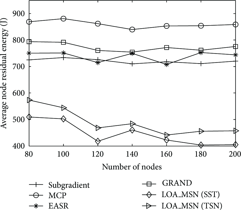
Average node residual energy comparison.

Subgradient algorithm uses the optimization algorithm to solve the model (17a) and obtain data routing scheme. It cannot calculate the number of hops of each sensor node. Therefore, Figure 8 compares the data gathering latency of MCP, EASR, GRAND, LOA_MSN (SSN), and LOA_MSN (TSN). LOA_MSN (TSN) reduces the communication distance with two mobile sink nodes. LOA_MSN (SSN) stays at some anchors surrounding the simulation area and increases the number of hops of sensor nodes which are far from sink node. In MCP, fixed sink node gathers data in the center of simulation area. In EASR and GRAND, sink node moves around the center of simulation area and uses MCP to gather data when sink node stays at one grid center. Therefore, LOA_MSN (TSN) has the lowest data gathering latency. Data gathering latency in MCP, EASR, and GRAND has little difference. LOA_MSN (SSN) has the largest data gathering latency.

Figure 8

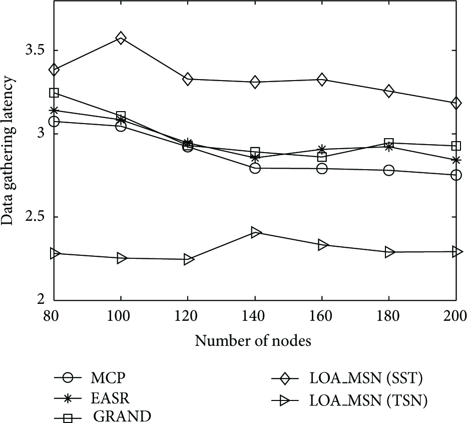
Data gathering latency comparison.

In summary, in the WSNs of uniformly distributed nodes, and LOA_MSN makes full use of node energy to prolong network lifetime. When LOA_MSN uses multiple sink nodes, it also reduces node energy consumption and data gathering latency.

5.2.2. WSNs of Nonuniformly Distributed Nodes

In the simulation, 3–5 numbers of points around the center of simulation area are generated as the mean parameters of Poisson distribution. The locations of 100 sensor nodes are Poisson randomly generated around the mean parameters. As is shown in Figure 9, in the 1000 m * 1000 m simulation area there are four mean points. 100 sensor nodes Poisson distribute around the four points. Namely, the nodes densely distribute around the four points. They sparsely distribute, even no node distributes in the regions which are far away from the four points. According to the node location information, LOA_MSN finds the centers of dense subregions, and obtains the five anchors (five-pointed stars). When sink nodes stay at those anchors, all sensor nodes have the opportunity to transmit data near their corresponding sink node.

Figure 9

Grid movement paths of two sink nodes when sensor nodes distribute nonuniformly.

Figure 10 compares the network lifetime when sensor nodes distribute nonuniformly. In the network of nonuniform node distribution, sensor nodes concentrate in several subregions. LOA_MSN successfully finds the center of each dense subregion and uses distributed synchronous Bellman-Ford algorithm to obtain the data transmission scheme which prolongs network lifetime. Network lifetime of other algorithms is affected by the network topology. The hub nodes in dense subregions forward a lot of data and are disable quickly. Therefore, as shown in Figure 10, LOA_MSN (TSN) has the longest network lifetime. LOA_MSN (SSN) has the second. Network lifetime of LOA_MSN has not been affected by the node locations and even increases compared with the network lifetime in the WSNs of uniformly distributed nodes. Other algorithms have low network lifetime.

Figure 10

Network lifetime comparison in the WSNs of nonuniformly distributed nodes.

In the WSNs of nonuniformly distributed nodes, the simulation results of average node energy consumption, average residual energy, and data gathering latency are similar to the simulation results in the WSNs of uniformly distributed nodes. Therefore, the results are not elaborated.

In summary, in the WSNs of nonuniformly distributed nodes, LOA_MSN makes full use of node energy to prolong network lifetime.

6. Conclusion

In the paper, lifetime optimization algorithm with mobile sink nodes for wireless sensor networks based on location information (LOA_MSN) is proposed. In the proposed scheme, satellite positioning and RSSI positioning algorithms are used to obtain the location information of all nodes. Then, the constraints are analyzed and movement path selection model and lifetime optimization model with known movement paths are established. Sink nodes gather the location information of sensor nodes and use the clustering method and graph theory method to find the movement paths. They stay at the grid centers which are in the movement path for some time, and gather data of sensor nodes with distributed method. Finally, the performances of MCP, subgradient algorithm, EASR, GRAND, and LOA_MSN are compared. It has been shown through various experiments that sink nodes find the appropriate paths. LOA_MSN makes full use of node energy to prolong network lifetime. When LOA_MSN uses multiple sink nodes, it also reduces node energy consumption and data gathering latency.