
Abstract
Due to the development and popularization of Internet, there is more and more research focusing on complex networks. Research shows that there exists community structure in complex networks. Finding out community structure helps to extract useful information in complex networks, so the research on community detection is becoming a hotspot in recent years. There are two remarkable problems in detecting communities. Firstly, the detection accuracy is normally not very high; Secondly, the assessment criteria are not very effective when real communities are unknown. This paper proposes an algorithm for community detection based on hierarchical clustering (CDHC Algorithm). CDHC Algorithm firstly creates initial communities from global central nodes, then expands the initial communities layer by layer according to the link strength between nodes and communities, and at last merges some very small communities into large communities. This paper also proposes the concept of extensive modularity, overcoming some weakness of modularity. The extensive modularity can better evaluate the effectiveness of algorithms for community detection. This paper verifies the advantage of extensive modularity through experiments and compares CDHC Algorithm and some other representative algorithms for community detection on some frequently used datasets, so as to verify the effectiveness and advantages of CDHC Algorithm.
1. Introduction
Complex networks are generally networks having lots of nodes and connections, such as Internet, citation network, and social network [1–3]. Due to Internet's development and popularization, there is more and more research on complex networks in recent years. Research shows that there exists community structure [4] in complex networks. Connections within a community are dense, while connections between different communities are rare [5]. Generally, a community consists of nodes having similar properties, so finding communities helps to mine some useful information of complex networks, for example, finding a group of people having common interests. How to detect communities in complex networks is a hotspot in recent years.
Newman and Girvan [6] put forward the conception of modularity to measure the quality of algorithms for community detection. The modularity Q is a number less than 1. The bigger Q is, the better quality is. Modularity has become the most widely used assessment criterion for community detection due to two reasons when we do not know the real communities in networks. Firstly, modularity is very convenient to use. Secondly, it seems that the result is better when the modularity is bigger in most cases. Many algorithms [7–9] detect communities by maximizing modularity. As it is impossible to calculate the modularity for every possible case, such kind of algorithms usually adopts greedy strategy to find the case almost maximizing modularity.
As modularity becomes more and more popular, people begin to doubt its effectiveness. Fortunato and Barthélemy [10] said algorithms based on modularity are not able to detect communities whose size is less than an inherent size depending on the number of networks’ edges. It is called by Fortunato the resolution limit of modularity. We find out by experiment that the quality is not necessarily better when the modularity is bigger. Maximizing modularity tends to detect more communities than the real situation, because the upper boundary of modularity is bigger when we detect more communities. In order to overcome this problem, this paper proposes the conception of extensive modularity on the basis of modularity. The upper boundary of extensive modularity is independent of the number of communities that we detect. We find out that the result maximizing extensive modularity is better than that maximizing modularity.
For now, there are many algorithms having advantages and disadvantages for community detection. Algorithms based on graph theory appear early, and their main idea is to divide the network into k such parts of almost the same size satisfying that connections in the same part are dense and connections between different parts are rare. Kernighan-Lin Algorithm [11] and bisection of spectrum based on Laplace eigenvalues [12] are representative algorithms based on graph theory. Generally speaking, it is hard to know the number of communities ahead of time, but algorithms based on graph theory need the number, so the accuracy is very low. Algorithms based on hierarchical clustering are common to see for now. This kind of algorithms decomposes datasets hierarchically according to a certain method until it satisfies some certain conditions. According to the principle of classification, algorithms based on hierarchical clustering can be divided into two parts, which are aggregation algorithm and splitting algorithm. GN Algorithm [6] is a representative splitting algorithm, while CNM Algorithm [13] and Newman Fast Algorithm [14] are representative aggregation algorithms. GN and CNM can usually obtain large value of modularity, while the accuracy is not necessarily high. LCV Algorithm [15] detects communities by finding local central vertices. EACH Algorithm [16] detects communities by calculating the edge antitriangle centrality with the isolated vertex handling strategy. LCV and EACH are both algorithms based on hierarchical clustering. Besides, there are also other kinds of algorithms.
The rest of this paper is organized as follows: Section 2 introduces some definitions including central nodes, nodes’ similarity, link strength between a node and a community, modularity, and extensive modularity; Section 3 describes detailed steps of the algorithm proposed by this paper; Section 4 states experiment results; the last section is our conclusion.
2. Definitions for Community Detection
Notation of Main Symbols gives the meaning of the main symbols that we will use in the whole paper.
2.1. Central Node
Central nodes include global central nodes and local central nodes. In a network, k nodes with maximal degree are called its global central nodes, in which the value of k can be determined according to our needs. If a node's degree is bigger than the degree of all its adjacent nodes, we call it local central nodes.
Global central nodes play an important role in the network and are probably important nodes of communities. So global central nodes help to find communities.
2.2. Nodes’ Similarity
We define the similarity of node a and node b as

Paper [16] defines the similarity of node a and node b as

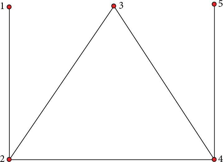
Network 1.
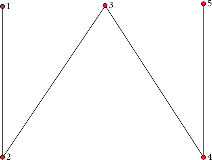
Network 2.
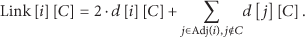
2.3. Link Strength between a Node and a Community
We define the link strength between node i and community
2.4. Modularity Q
The modularity Q is defined as

Q is a number less than 1. The bigger Q is, the better algorithm's quality is. The quality is generally good when Q is between 0.3 and 0.7. Q is difficult to exceed 0.7 in the real situation.
2.5. Extensive Modularity
We define extensive modularity


Through (6), we can know that
3. Algorithm Description
One city has one or several centers and is expanded layer by layer around the centers. The closer to the center the layer is, the denser the connections to the layer are. The outer layer is connected mainly by itself and inner layers. Inspired by the hierarchical structure of cities, we consider that a community should have one or several global central nodes and should be expanded layer by layer around the global central nodes. The nodes in layer p are mainly connected by nodes in layer p and layer
We suppose the network is connected, which means we can reach any node from any node through some edges in the network.
3.1. Initialize Communities
The process of initializing communities can be divided into three steps, which are sorting nodes, choosing global central nodes, and merging global central nodes into communities.
Step 1.
Sort all the nodes by degree in descending order.
Step 2.
Choose k nodes with maximal degree as global central nodes of the network. The value of k is determined by the following equations:

The idea is that we want to choose a small number of global central nodes to reduce the quantity of calculation and the global central nodes include the important nodes of each community. If there are only a small number of nodes with large degree and the degree of most nodes is small, we generally have
Step 3.
Initialize the first community, assign the node with maximal degree to the first community, and then mark it as the first community's central node. For each node v of the remaining
Algorithm 1 shows the process of initializing communities.
sort nodes by degree in descending order; choose k global central nodes initialize community nc = 1; //nc: number of communities; assign mark calculate sim( mark maximal sim and its pos; nc++; initialize C[nc]; assign mark assign
3.2. Expand Communities
After finishing the process of initializing communities, we need expand these communities. The process of expanding communities includes marking nodes’ level and calculating link strength.
Step 1.
Mark all the global central nodes of the network as the first level. If the node v is connected to a node of the first level and its level is not marked, mark its level as two. If the node v is connected to a node of level p and its level is not marked, mark its level as
Step 2.
Nodes of the first level have already been assigned to communities. For each node v of level two, we calculate the link strength between the node v and each community C. Choose the community maximizing the link strength and then assign the node v to it. By parity of reasoning, for each node v of level, we repeat the previous operation, until every level's nodes have been assigned to communities.
Algorithm 2 shows the process of expanding communities.
add lev[j] = lev[i] + 1; add j to stack; sort nodes by level in ascending order; calculate link[v][C[i]]; mark maximal link and its pos; assign to C[max_pos];
3.3. Merge Small Communities
After the previous two processes, every node is assigned to a community. Some communities are probably of very small size, and we need to merge these communities into the other communities. This process includes determining small communities and calculating the number of common nodes.
Step 1.
If a community is of size smaller than t, we call it small community; otherwise, we call it large community. The value of t is determined by the following equation:

Step 2.
When merging communities, we will not merge a whole community into another one, because not all the nodes are strongly connected to the same community. We will merge small communities node by node into large communities. For each node v in small communities, calculate the number of common nodes of the node v's adjacent nodes and each large community. If the node v's adjacent nodes have the most common nodes with the community C, reassign the node v to community C.
Algorithm 3 shows the process of merging little communities.
determine little communities and large communities; calculate the number of common nodes; between adj(v) and C; mark the pos of the largest number; reassign v to C[max_pos];
3.4. Choose the Best Result
Given a network, we will detect its communities after the previous three processes. In the process of initializing communities, we give the threshold η of similarity. Different threshold will lead to different result. The smaller the threshold η is, the more likely the two global central nodes are assigned to the same community, so there tend to be fewer communities. We need to choose an appropriate value of threshold η so as to detect the real number of communities and get the best result.
For the threshold η, take at regular interval ten values from 0.1 to 1, and repeat the previous three processes for each value. Then we obtain ten partitions of the network. Generally, we are not able to know the real communities, so we have to choose the best result through an assessment criterion. For now, modularity is the most widely used criterion. However, we find that the result maximizing the extensive modularity is usually better than the result maximizing the modularity and conforms to the real situation very well. So we choose the partition with maximal value of extensive modularity as the best result.
Now we analyze the time complexity of CDHC. The first process costs
4. Experiments
Firstly, we choose three most widely used datasets, which are Zachary Karate Club [17], Dolphin Network [18], and American College Football [19]. Secondly, we introduce some assessment criteria used in the case that the real communities are known. Thirdly, we verify the advantage of extensive modularity on the three datasets. Lastly, we choose some classical or new algorithms and compare them with CDHC on the three datasets.
4.1. Datasets
4.1.1. Zachary Karate Club
It is a social network of friendships between 34 members of a karate club at a US university in the 1970s. A factional division leads to a formal separation of the club into two organizations of nearly equal size.
4.1.2. Dolphin Network
It is an undirected social network of frequent associations between 62 dolphins in a community living off Doubtful Sound in New Zealand. It contains totally 62 dolphins in two groups.
4.1.3. American College Football
It is a network of American football games between Division IA colleges during regular season fall 2000. It contains 115 teams, which are divided into 12 conferences, each containing 8 to 12 teams.
Table 1 is a summary of the three datasets’ basic information, including NOC (number of communities), number of nodes, and number of edges.
Dataset information.

4.2. Assessment Criteria
Given a network G,
4.2.1. Precision [20]
Precision is defined as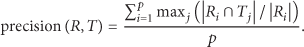
4.2.2. Recall [20]
Recall is defined as 
4.2.3. F-Measure [21]
F-measure is defined as
4.2.4. NMI [22] (Normalized Mutual Information)
NMI is defined as
According to our discussion about the four criteria, we will take F-measure and NMI to evaluate the result of community detection.
4.3. Experimental Results on Extensive Modularity
For the threshold η, we take at regular interval ten values from 0.1 to 1, and we obtain ten different partitions, respectively, on the datasets Zachary, Dolphin, and Football. For each partition, we use NOC (number of communities), modularity Q, extensive modularity
Table 2 is the ten experimental results under different threshold η on the dataset Zachary. Seen from the modularity, the best result should be the case when the threshold is 0.6. We can see that the maximal value of modularity is 0.373. In this case, we find that the detected communities differ much from the real communities. The detected NOC is 3, while real NOC should be 2. Besides, the value of F-measure and NMI is not very high. Seen from extensive modularity, the best result is the case when the threshold is 0.2. The maximal value of extensive modularity is 0.744. In this case, the values of F-measure and NMI are both 1, which signifies the detected communities are exactly the same with the real communities.
Experimental results under different threshold η on the dataset Zachary.
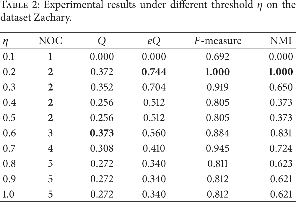
Table 3 is the ten experimental results under different threshold η on the dataset Dolphin. Seen from the modularity, the best result is the case when the threshold is 0.3. We can see that the maximal value of modularity is 0.477. In this case, we find that the detected communities also differ much from the real communities. The detected NOC is 4, while real NOC should be 2. Besides, the value of F-measure and NMI is very low. Seen from extensive modularity, the best result is the case when the threshold is 0.2. The maximal value of extensive modularity is 0.770. In this case, the values of F-measure and NMI are very close to 1, which signifies the detected communities are very close to the real communities. Though maximizing extensive modularity does not find the best result, it is very close to the best result and is far better than the case maximizing modularity.
Experimental results under different threshold η on the dataset Dolphin.

Table 4 is the ten experimental results under different threshold η on the dataset Dolphin. Seen from modularity or extensive modularity, the best result is the case when the threshold is 0.5. In this case, the detected NOC is 11, which is very close to the real NOC 12. We see that maximizing modularity or extensive modularity does not find the best result, but it has only a slight gap with the best result.
Experimental results under different threshold η on the dataset Football.

From the discussion on the experimental results on the three datasets, the result maximizing extensive modularity usually is the best result or very close to the best result, while the result maximizing modularity is usually not very good. We can thus consider that extensive modularity is a better criterion compared to modularity.
4.4. Experimental Results on Comparison of Algorithms
As we have discussed, the extensive modularity is a better criterion than modularity, so we choose the case maximizing extensive modularity as the best result and the final result. We have chosen four algorithms for comparison, which are GN Algorithm [6], CNM Algorithm [13], EACH Algorithm [16], and LCV Algorithm [15].
Table 5 is the experimental results of the five algorithms on the dataset Zachary. GN and CNM get large value of modularity, but they detect more communities than the real situation, and their value of NMI is very low. EACH, LCV, and CDHC have detected the real communities. So EACH, LCV, and CDHC are far better than GN and CNM on Zachary.
Experimental results of algorithms on the dataset Zachary.

Table 6 is the experimental results of the five algorithms on the dataset Dolphin. GN, CNM, and EACH get large value of modularity, but they detect more communities than the real situation, and their value of NMI is very low. LCV and CDHC get large value of extensive modularity, and the detected communities are very close to the real communities. LCV and CDHC are far better than GN, CNM, and EACH on Dolphin. Furthermore, CDHC is slightly better than LCV.
Experimental results of algorithms on the dataset Dolphin.
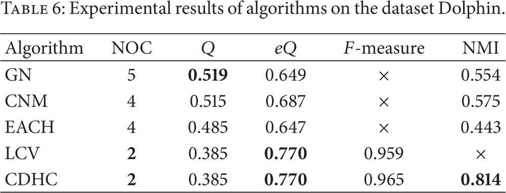
Table 7 is the experimental results of the five algorithms on the dataset Football. The modularity of the five algorithms differs a little. The NOC detected by GN and CNM is far less than the real NOC 12. GN gets the largest value of extensive modularity, but its NMI is relatively low. CDHC gets the second largest value of extensive modularity, and its NMI is very close to the best result. On the whole, EACH and CDHC are better on Football.
Experimental results of algorithms on the dataset Football.

From the experimental results on the three datasets, we find that GN and CNM usually get large modularity. However, the detected communities usually differ much from the real communities. Large NOC makes it easy to get a large modularity. CDHC usually gets large extensive modularity, and the detected communities are very close to the real communities. On the whole, CDHC is far better than GN and CNM and is slightly better than EACH and LCV.
Figures 3, 4, and 5 show the communities that CDHC has detected on Zachary, Dolphin, and Football. We can see that the community structure is evident.

Communities detected of Zachary.

Communities detected of Dolphin.
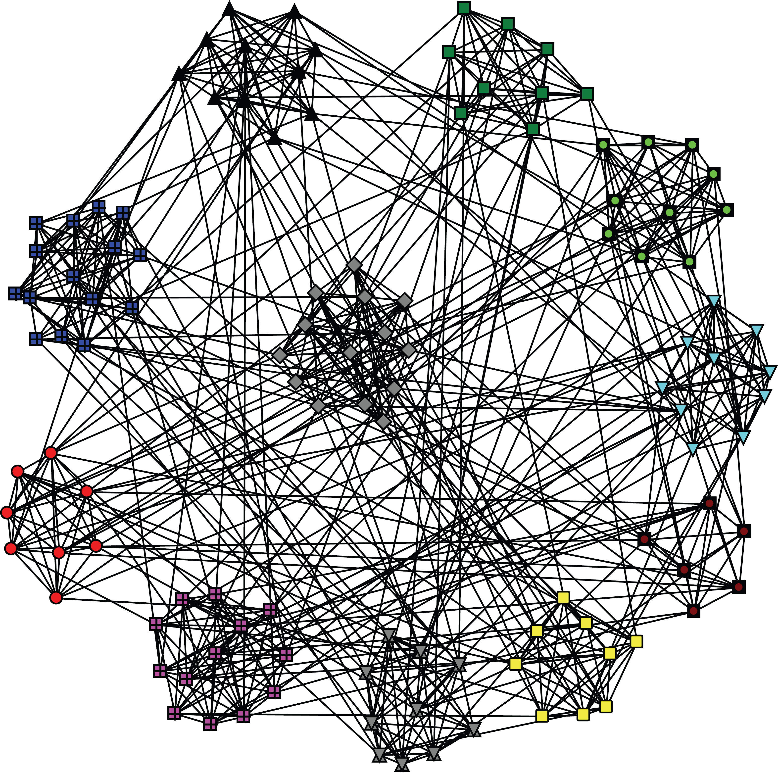
Communities detected of Football.
5. Conclusion
This paper proposes the conception of extensive modularity on the basis of modularity. The upper boundary of extensive modularity is independent on the number of communities that we detect, so it overcomes the weakness of modularity that maximizing modularity tends to detect more communities than the real situation. We verify through experiments that extensive modularity is a better criterion than modularity when the real communities are unknown.
This paper proposes CDHC Algorithm. CDHC Algorithm includes four processes, which are initializing communities, expanding communities, merging little communities, and choosing the best result. We choose four algorithms to compare with CDHC on three datasets, which are Zachary, Dolphin, and Football. We find that CDHC is far better than GN and CNM and is slightly better than LCV and EACH. According to F-measure and NMI, the communities detected by CDHC are very close to the real communities.
Footnotes
Notation of Main Symbols
Conflict of Interests
The authors declare that there is no conflict of interests regarding the publication of this paper.
Acknowledgments
The work is supported by National Natural Science Foundation of China (no. 61402028) and Science Foundation of Shenzhen City in China (JCYJ20140509150917445).