Multitarget Tracking by Particle Filtering Based on RSS Measurement in Wireless Sensor Networks

Abstract

We propose an algorithm for multitarget tracking by particle filtering in wireless sensor networks based on received signal strength (RSS) measurement where we also localize a newly appearing target whose location and reference power are unknown. Therefore, the number, the reference power, and the initial locations of targets are unknown in this problem. At the initial localization step, we apply approximate least squares (LS) method to roughly estimate the target location. After the initial location is estimated, we estimate the reference power. This is possible because we can use multiple number of measurements for estimating multiparameters. The proposed approach is particularly emphasized on the initialization step that completes the whole multitarget tracking system by particle filtering in a challenging scenario. The proposed approach is validated by computer simulations for its effectiveness.

1. Introduction

In wireless sensor networks, we can take advantage of many sensors to estimate certain states of targets. In this paper, we propose an algorithm to detect and track targets based on the received signal strength (RSS) measurement where an unknown number of targets vary with time, and the “reference power” of the targets is also unknown and varies with time. In fact, RSS measurement model is not very popular in the literature regarding target tracking or target localization [1, 2] because, whereas bearing and/or range measurement provides one-to-one mapping between a measurement and a parameter of interest, RSS measurement generally does not provide one-to-one mapping except for the cases when the measurement is obtained over the sensor fields by using “a grid spacing” and when “standard commercial radio-frequency (RF) prediction tools” are used. Therefore, we do not assume “one-to-one” mapping between a measurement and a target in this paper. A salient feature of the RSS measurement is that the parameter to be estimated is directly related with the measurement while bearing and/or range measurement is not. This means that the data fusion methods, such as time of arrival (TOA) [3], time difference of arrival (TDOA) [4–6], or angle of arrival (AOA) [7, 8], require a preprocessor before acquiring the measurement (bearing or range) while RSS [9–11] is almost raw data from the target. Therefore, we might be able to apply maximum likelihood (ML) method directly to RSS measurement-based estimator.

The least squares (LS) method is successfully employed for localization methods using the data fusion methods, for example, TOA, TDOA, AOA, and RSS, specifically, in a mobile locating systems [12, 13] or sensor node localization in a wireless ad hoc sensor networks [14]. Interestingly, a maximum likelihood (ML) method can be applied to the RSS model to improve the performance beyond the LS method [15]. Once a target is identified, particle filtering can be applied to track the dynamic states of the target. The problem of multitarget tracking is not an easy task while various approaches, for example, extended Kalman filter, data fusion, and joint probabilistic data association, were proposed in the literature [16–21].

We assume that the initializing step is applied to only a new single target identification. First, we directly estimate the distance between a possible new target and each sensor based on measurements and formulate the equation with respect to the squared-estimated-distance for each sensor. And then we can cancel out the quadratic part of equations before applying linear LS method. After initializing the location of the new possible target, we estimate the reference power given the estimated location when the reference power is unknown. The contributions of the paper consist in proposing an algorithm for multitarget tracking in wireless sensor networks where initial positions of targets, the reference power of the targets, the number of targets are unknown and estimated. A number of statistical approaches are jointly employed in this algorithm such as least squares method, iterative maximum likelihood method, and particle filtering. The challenge consists in tracking multitargets based on a single signal strength transmitted from targets.

This paper is organized as follows. In the following section, the problem is formulated in a mathematical model. Next, we show how to initialize targets. The initialization process is described for both cases of known reference power and unknown reference power. And then particle filtering is described for tracking varying number of targets. The computer simulations to verify the validity of the proposed algorithm follow. The paper is concluded at the final section.

2. System Model

2.1. Measurement and State Space Model

We consider a $\mathrm{2}$ D rectangular field of interest with uniformly distributed sensors. The RSS measurement at the sensor n from source targets at the time step k is described as follows [22]:

$$\begin{array}{l}{y}_{n,t}=\mathrm{10}\hspace{0.17em}{\log }_{\mathrm{10}}\left({\displaystyle \sum }_{k=\mathrm{1}}^K‍\frac{{\Psi }_k{d}_{\mathrm{0}}^{\alpha }}{{\left|{\mathbf{r}}_n-{\mathbf{l}}_{k,t}\right|}^{\alpha }}\right)+v_{n,t},\\ \phantom{\mathrm{10}{\log }_{\mathrm{10}}\left({\displaystyle \sum }_{k=\mathrm{1}}^K‍\mathrm{5552}\right)}n=\mathrm{1,2},\dots ,N,\end{array}$$

(1)

where ${\mathbf{l}}_{k,t}$ is the location of the target k at the time step t, n is the sensor index, K is the number of targets, ${\Psi }_k$ is the reference power of the target k, that is, the received power from the source at the reference distance $d_{\mathrm{0}}$ , r is the sensor location, α is the attenuation factor ( $\alpha \ge \mathrm{1}$ ), v is the background zero-mean Gaussian noise, and N is the total number of sensors used in the field. The RSS measurement model does not provide much information about targets, for example, the number of targets, the distance from sensors, and the direction of the source. We use three or four best sensors, that is the three strongest received signals when we apply the LS method with known reference power while four best measurements are employed with unknown reference power for initialization of a newly appearing target. In the tracking system, we have to be able to estimate the location and the reference power of targets, in addition to the number of targets at every time step based on a single “signal strength” at each sensor, which is a challenging problem.

We model a single moving target system by a linear state space model as follows [1, 18, 23]:

$$\begin{array}{cc}& {\mathbf{x}}_t={\mathbf{f}}_t({\mathbf{x}}_{t-\mathrm{1}},{\mathbf{u}}_t)={\mathbf{G}}_x{\mathbf{x}}_{t-\mathrm{1}}+{\mathbf{G}}_u{\mathbf{u}}_t,\end{array}$$

(2)

where ${\mathbf{x}}_t={\left[\begin{array}{cccc}{x}_{\mathrm{1},t}& x_{\mathrm{2},t}& {\dot{x}}_{\mathrm{1},t}& {\dot{x}}_{\mathrm{2},t}\end{array}\right]}^{\top }$ is the state vector which indicates the position and the velocity of a target, respectively, in a 2D Cartesian coordinate system. ${\mathbf{G}}_x$ and ${\mathbf{G}}_u$ are known matrices according to the classical dynamics defined by

$$\begin{array}{cc}& {\mathbf{G}}_x=\left(\begin{array}{cccc}\mathrm{1}& \mathrm{0}& T_s& \mathrm{0}\\ \mathrm{0}& \mathrm{1}& \mathrm{0}& T_s\\ \mathrm{0}& \mathrm{0}& \mathrm{1}& \mathrm{0}\\ \mathrm{0}& \mathrm{0}& \mathrm{0}& \mathrm{1}\end{array}\right),\hspace{1em}\hspace{1em}{\mathbf{G}}_u=\left(\begin{array}{cc}\frac{T^{\mathrm{2}}}{\mathrm{2}}& \mathrm{0}\\ \mathrm{0}& \frac{T^{\mathrm{2}}}{\mathrm{2}}\\ T_s& \mathrm{0}\\ \mathrm{0}& T_s\end{array}\right).\end{array}$$

(3)

$\mathbf{u}={\left[\begin{array}{cc}{\ddot{x}}_{\mathrm{1},t}& {\ddot{x}}_{\mathrm{2},t}\end{array}\right]}^{\top }$ , where u is the Gaussian noise-like acceleration perturbation and $T_s$ is sampling time-period (s). Targets maneuver with random acceleration based on classical dynamics (discrete-time version). Only a part of the state is related with the measurement in the RSS model because the state comprises location and velocity while only the location of a target contributes to the measurement. Nevertheless, once we estimate any one of them, we can relate them and find the rest of the states since all states are related by classical mechanics. The Doppler effect should be taken into account for a target with considerably high speed in a real scenario in order to obtain enhanced performance.

2.2. Varying Pattern of the Number of Targets

We use particle filtering to track the variable and multiple number of targets in this paper. At any time step, particles are propagating according to the dynamic state space model. We assume a certain pattern by which the number of targets varies between two consecutive time steps. We assume that the number of targets varies according to three patterns as follows [24].

• (1)

The number of targets remains the same as at the previous time step with the same identities.

(2)

The number of targets increases by a newly appearing target.

(3)

The number of targets decreases by one, that is, in the tracked targets at the previous time step.

If the sampling time-period for the discretization is short enough, the above assumption will be satisfied.

3. Initializing a Single Target with Known Reference Power

The approximate LS method is not the best performing method for the localization [15]. However, if we use particle filtering for target tracking, a fast and simple initializing method can be more efficient (as LS method does) rather than a complicated and highly accurate method because particle filtering will retrieve the right track eventually even with a low-accuracy location-estimate. Therefore, we jointly employ the approximate LS method and particle filtering for initialization and tracking, respectively. Generally, the prior distribution of a target, that is, the probabilistic distribution of the target, is assumed to be known in the application of particle filtering.

3.1. Least Squares Method

Let us suppose that we have $\mathfrak{m}$ unknowns and $\mathfrak{n}$ linear equations, and we can describe the problem by the equations as follows:

$$\begin{array}{cc}& H\mathbf{x}=d,\end{array}$$

(4)

where H is a $\mathfrak{n}$ -by- $\mathfrak{m}$ , x is a $\mathfrak{m}$ -by-1, and d is a $\mathfrak{n}$ -by-1 matrices, respectively. Depending on the sizes of $\mathfrak{m}$ and $\mathfrak{n}$ , we can consider the problem in three cases. If $\mathfrak{m}>\mathfrak{n}$ , we have a smaller number of equations than that of unknowns. In this case the solution is underdetermined or incompletely specified. In this case, there are many solutions that satisfy the above equation. An approach to this case is known to be minimum norm solution that has the criterion as follows:

$$\begin{array}{cc}& \min ‖\mathit{x}‖\hspace{1em}\text{such}\mathrm{\hspace{0.17em}\hspace{0.17em}}\text{that}\hspace{0.17em}\hspace{0.17em}H\mathit{x}=d.\end{array}$$

(5)

If the rank of H is $\mathfrak{n}$ , then $H{H}^{\top }$ is invertible, and a solution can be obtained as follows:

$$\begin{array}{cc}& H^{\top }{\left(H{H}^{\top }\right)}^{-\mathrm{1}}d,\end{array}$$

(6)

where $H^{\top }(H{H}^{\top }{)}^{-\mathrm{1}}$ is called pseudoinverse of H for the underdetermined problem. If $\mathfrak{n}=\mathfrak{m}$ , H is a square matrix, and, unless H is singular, we can obtain a unique solution by using the inverse of H as follows:

$$\begin{array}{cc}& \mathit{x}=H^{-\mathrm{1}}d.\end{array}$$

(7)

Nonetheless, if H is singular, then we have no solution or many solutions.

Finally, if $\mathfrak{m}<\mathfrak{n}$ , we have a bigger number of equations than that of unknowns. In this case the equations are inconsistent and the solution is overdetermined. In this case, no solution exists that satisfies all of $\mathfrak{n}$ equations. Therefore, our concern is now to find x of the best approximation that is close to a solution in terms of least squared errors for all $\mathfrak{n}$ equations. The criterion of this approach is to minimize the norm of errors, which is described as follows:

$$\begin{array}{cc}& \min {‖\mathit{e}‖}^{\mathrm{2}}=\min {‖d-H\widehat{\mathit{x}}‖}^{\mathrm{2}}.\end{array}$$

(8)

The error vector satisfies the following orthogonal condition:

$$\begin{array}{cc}& H^{\top }\mathit{e}=\mathrm{0}.\end{array}$$

(9)

Then, the following is satisfied:

$$\begin{array}{cc}& H^{\top }H\widehat{\mathit{x}}=H^{\top }d.\end{array}$$

(10)

If H has full rank, then $H^{\top }H$ is invertible, and the least squares solution can be obtained as follows:

$$\begin{array}{cc}& \widehat{\mathit{x}}={\left(H^{\top }H\right)}^{-\mathrm{1}}{H}^{\top }d,\end{array}$$

(11)

where $(H^{\top }H{)}^{-\mathrm{1}}{H}^{\top }$ is the pseudoinverse of the matrix H for the overdetermined problem. Therefore, linear least squares solution can be obtained in the overdetermined problem. Please note that pseudoinverse has different forms depending on whether the problem is underdetermined or overdetermined. Furthermore, both formulations of pseudoinverse are identical with the exact inverse of a matrix when $\mathfrak{m}=\mathfrak{n}$ (on condition that H is not singular). Therefore, as long as we have two or more linear equations with two unknowns, least squares method can find either “exact solution” or “an approximate solution in terms of minimized norm of errors.”

In this paper, we have two or more number of equations than the number of unknowns (i.e., two). We need three measurements of quadratic equations in order to obtain two linear equations. Besides, we need four quadratic equations of measurements to obtain two linear equations when unknown reference power is jointly estimated.

We can use sensor measurements as many as we want. However, the signal to noise ratio decreases drastically as the distance increases between a sensor and a target. On the other hand, there is an ambiguity about better information among a number of measurements, particularly, between the second, the third, and the fourth. This is why we may want to employ more linear equations than that of unknowns sometimes while we need two linear equations most of the time in this paper. In this case, we need to obtain pseudoinverse for overdetermined problem. As shown in [25], increased number of linear equations improves the performance significantly for the case of “time-of-arrival (TOA)” or “time-difference-of-arrival” measurement while it is less effective for the problem employing RSS measurement. As a matter of fact, we do not need more than two linear equations because the information beyond two is redundant and even degrades the performance due to low SNR most of the time. Therefore, we use three sensor measurements with known reference power and four sensor measurements with unknown reference power.

From (1), we estimate the squared distance between sensors and a target location before applying the LS method when we assume $\alpha =\mathrm{2}$ and $d_{\mathrm{0}}=\mathrm{1}$  m (omitting the time index) as follows:

$$\begin{array}{cc}& {\left|{\mathit{r}}_n-\mathit{l}\right|}^{\mathrm{2}}\triangleq {{\rm Y}}_n^{\mathrm{2}}=\Psi {\left({\mathrm{10}}^{y_n/\mathrm{10}}\right)}^{-\mathrm{1}}.\end{array}$$

(12)

If we denote the estimated distances by $r_A$ , $r_B$ , and $r_C$ and corresponding locations of three sensors by $A(a_{\mathrm{1}},a_{\mathrm{2}})$ , $B(b_{\mathrm{1}},b_{\mathrm{2}})$ , and $C(c_{\mathrm{1}},c_{\mathrm{2}})$ , respectively, the LS method solves the equations as follows:

$$\begin{array}{cc}& H\mathbf{x}=d,\hspace{1em}\text{then}\mathrm{\hspace{0.17em}\hspace{0.17em}}\widehat{\mathbf{x}}={\left(H^{\top }H\right)}^{-\mathrm{1}}{H}^{\top }d,\end{array}$$

(13)

where

$$\begin{array}{cc}& H=\left[\begin{array}{cc}\mathrm{2}\left(a_{\mathrm{1}}-c_{\mathrm{1}}\right)& \mathrm{2}\left(a_{\mathrm{2}}-c_{\mathrm{2}}\right)\\ \mathrm{2}\left(b_{\mathrm{1}}-c_{\mathrm{1}}\right)& \mathrm{2}\left(b_{\mathrm{2}}-c_{\mathrm{2}}\right)\end{array}\right],\\ d=\left[\begin{array}{c}{a}_1^2-c_1^2+a_2^2-c_2^2+r_C^2-r_A^2\\ b_1^2-c_1^2+b_2^2-c_2^2+r_C^2-r_B^{\mathrm{2}}\end{array}\right],\end{array}$$

(14)

and $(H^{\top }H{)}^{-\mathrm{1}}{H}^{\top }$ is the pseudoinverse of H, and $\mathbf{x}={\left[\begin{array}{cc}x& y\end{array}\right]}^{\top }$ is the initialized target location. In order to obtain linear equations, we need to remove the quadrature part of equations by using the formulation of “ $r_C^2-r_A^2$ ” and “ $r_C^2-r_B^{\mathrm{2}}$ .” Therefore, we need three measurements to obtain two linear equations for estimating 2D position. Similarly, we need four measurements in order to apply this approach for estimating 3D position. The performance assessment of the LS initial localization is presented in the following section.

3.2. Performance of Initial Localization

In this section, we assess the performance of the LS and the ML methods in initial localization. These two methods have different features. Whereas the LS method does not consider any probabilistic assumptions, the ML method solves the problem in a probabilistic manner. Therefore, the ML approach finds the solution that maximizes the probability density function (PDF) given the measurement as follows:

$$\begin{array}{l}\ln p_y(\mathbf{y};\mathbf{l})\\ \hspace{1em}=\ln \left\{\frac{\mathrm{1}}{{\left(\mathrm{2}\pi {\sigma }^{\mathrm{2}}\right)}^{N/\mathrm{2}}}{e}^{\left\{-(\mathrm{1}/\mathrm{2}{\sigma }^{\mathrm{2}})\sum ‍{\left[y_n-\mathrm{10}{\log }_{\mathrm{10}}\left(C/{\mathbf{D}}_n\right)\right]}^{\mathrm{2}}\right\}}\right\},\end{array}$$

(15)

where $\Psi d_{\mathrm{0}}^{\alpha }=C$ , $\alpha =\mathrm{2}$ , $|{\mathbf{r}}_n-\mathbf{l}{|}^{\alpha }={\mathbf{D}}_n$ , and $\mathbf{y}={\left[\begin{array}{ccc}{y}_{\mathrm{1}}& y_{\mathrm{2}}& y_{\mathrm{3}}\end{array}\right]}^{\top }$ because we use only 3 measurements. Consequently, the ML method finds the value by which the first-order derivative of the log likelihood function becomes zero as follows:

$$\begin{array}{cc}& \frac{\partial \ln p(\mathbf{y};\mathbf{l})}{\partial \mathbf{l}}=\mathrm{0}.\end{array}$$

(16)

Because a solution in the closed form does not exist for the above equation, we need to apply an iterative method (i.e., the Newton-Raphson method) to find l that satisfies (16) as follows:

$$\begin{array}{cc}& {\mathbf{l}}_{k+\mathrm{1}}={\mathbf{l}}_k-{\left[\frac{{\partial }^{\mathrm{2}}}{\partial {\mathbf{l}}^{\mathrm{2}}}\left({\mathbf{d}}^{\top }\mathbf{y}-\frac{\mathrm{1}}{\mathrm{2}}{\mathbf{d}}^{\top }\mathbf{d}\right)\right]}^{-\mathrm{1}}{\left.\frac{\partial }{\partial \mathbf{l}}\left({\mathbf{d}}^{\top }\mathbf{y}-\frac{\mathrm{1}}{\mathrm{2}}{\mathbf{d}}^{\top }\mathbf{d}\right)\right|}_{\mathbf{l}={\mathbf{l}}_k},\end{array}$$

(17)

where d is defined in Appendix A, and the solution is derived therein. In the ML approach, we adopt the solution of the LS method as an initial guess ( ${\mathbf{l}}_{\mathrm{0}}$ ). Therefore, the ML approach certainly requires more steps beyond the LS method. We also compare the performances of these methods with Cramer-Rao bound (CRB) which is derived in Appendix B. When we apply the iterative method, we have to be careful because it can diverge sometimes, especially when the second-order derivative of the log-likelihood function is small [26]. Therefore, in the simulation, we set the threshold for the second-order derivative such that when inverse of derivative is larger than the threshold, it stops the iteration and adopts the LS estimate as the solution in order to avoid the divergence. We select $\mathrm{10}$ as the iteration number. The number of iterations was selected after extensive simulations with various values of iteration numbers. The performance was improved clearly as we increased the iteration number up to $\mathrm{5}$ in the computer simulations while, sometimes, we have enhanced performance with values greater than $\mathrm{5}$ . Therefore, we safely select $\mathrm{10}$ as the iteration number for assuring that we do not obtain improved performance any more.

The $\mathrm{2}$ D locating system field is depicted in Figure 1. The length of both sides of the field is $\mathrm{200}$  (m), respectively. The number of networked sensor nodes is $\mathrm{5}$ -by- $\mathrm{5}$ = $\mathrm{25}$ . The value of $\mathrm{1}\times \mathrm{1}{\mathrm{0}}^{\mathrm{4}}$  (J/s) is selected for the known reference power which can be known in practical situation (e.g., the reference power of mobile phones or anchor nodes is known). The values for $\alpha =\mathrm{2}$ and $d_{\mathrm{0}}=\mathrm{1}$ are selected for simulations. In the simulations, a number of different locations of the targets are estimated. The source targets are located at (20,20), (130,10), (140,140), (20,150), and (200,200), respectively. The number of performed simulations is $\mathrm{1000}$ , and background noise is chosen by three different values ( $\mathrm{0.01}$ , $\mathrm{0.1}$ , and $\mathrm{0.2}$  [dB]). We assume that the noise power is specified in dBW and that the unit of measure for the noise is volts. For power calculations, it is assumed that there is a load of 1 ohm. If we compare each pair of the result when the target is located at (20,20), Figures 2–4 show that the ML method compresses the distribution of LS estimates more densely around the true value. Some of ML iterative estimates have relatively larger errors. This is because the ML iterative estimates diverge sometimes. We stop the iteration and employ the LS estimate in this case.

Figure 1

$\mathrm{2}$ -dimensional field of locating system.

Figure 2

Estimated positions of the target when noise power is $\mathrm{0.01}$  dB.

Figure 3

Estimated positions of the target when noise power is $\mathrm{0.1}$  dB.

Figure 4

Estimated positions of the target when noise power is $\mathrm{0.2}$  dB.

The simulation results are shown in Figures 5–7 where the values are averaged for results with respect to various locations of the targets. Figure 5 shows the mean of distance error of two methods. As it shows, the iterative ML method outperforms the LS method. In Figures 6-7, the performances of two methods are compared to the CRB. The CRB is a lower-bound for the variance of estimates of an arbitrary unbiased estimator. When the noise power is low (0.01 dB), the ML iterative method obtains performance almost the same as the CRB. The exact values of the simulation results are summarized in Table 1. For example, when the noise power is 0.01 dB, the mean of distance error of the LS method is $\mathrm{1.38}$  m, $\mathrm{0.44}$  m for the iterative ML method, the CRB in X-coordinate is 0.16 m², the variance of the realized estimates in X-coordinate for the LS method is 1.19 m², and the variance of the realized estimates in X direction for iterative ML method is 0.13 m², respectively. It shows that the variance of the estimates for the iterative ML method is below the CRB when the noise power is 0.01 dB, which means that the iterative ML estimator is not unbiased. The bias is caused since we approximated the ML estimator by the numerical iterative method, and, furthermore, our ML estimator does not have a large data record for measurement to be asymptotically optimal. We can see the highly improved performance by the ML approach compared to that of the linearized LS method as shown in the results.

Table 1

The result of simulation, MED, mean error distance, CRB, Cramer-Rao bound, X, X coordinate, Y, Y coordinate, LS, least squares, and ML, maximum likelihood.

Noise power [dB]	MED-LS [m]	MED-ML [m]	CRB-X [m2]	CRB-Y [m2]	Var-LS-X [m2]	Var-LS-Y [m2]	Var-ML-X [m2]	Var-ML-Y [m2]	SNR [dB]
0.01	1.38	0.44	0.16	0.16	1.19	1.25	0.13	0.14	38.38
0.1	4.52	1.45	1.58	1.58	12.79	12.88	2.12	1.66	28.38
0.2	14.19	10.57	16.77	16.76	138.21	131.39	111.14	99.70	18.29

Figure 5

Mean of distance error by two methods.

Figure 6

Comparison between CRB and variances by two methods, X coordinate.

Figure 7

Comparison between CRB and variances by two methods, Y coordinate.

3.3. Least Squares for Multitargets

One of the most difficult scenarios in target tracking problem arises when the multiple number of targets varies. The LS method needs to be modified to be applied when the number of targets varies. We suppose that the number of targets varies following the varying pattern as specified at the beginning of Section 2.2. If there are targets being tracked, and an additional target appears, we reformulate the measurement equations with respect to the distance between the new target and each sensor. Then, we apply the approximate LS method to the newly formulated equations. The whole procedure for initializing a new target is described in Algorithm 1.

Algorithm 1 (initializing a new target in multitargets via least squares method (with known reference power).

(i) We suppose the number of sensors in the field is N, and the number of continuing targets is K. At any time step, we receive the measurements $y_{\mathrm{1}:N}$ as follows and we define

$$\begin{array}{l}{y}_n=10{log}_{10}\left(\sum _{k=1}^{K+1}\frac{{\psi }_k{d}_0^{\alpha }}{|r_n-1_k{|}^{\alpha }}\right)+v_n\hfill \\ \hspace{0.17em}\hspace{0.17em}\hspace{0.17em}\hspace{0.17em}\triangleq 10{log}_{10}\left[\left(\sum _{k=1}^K\frac{{\psi }_k{d}_0^{\alpha }}{|r_n-1_k{|}^{\alpha }}\right)+\frac{{\psi }_{K+1}{d}_0^{\alpha }}{|r_n-1_{K+1}{|}^{\alpha }}\right]\hfill \\ \hspace{0.17em}\hspace{0.17em}\hspace{0.17em}\hspace{0.17em}\triangleq 10{log}_{10}\left[{\Gamma }_n+\frac{{\psi }_{K+1}{d}_0^{\alpha }}{{\gamma }_n^{\alpha }}\right],\hspace{0.17em}\hspace{0.17em}\hspace{0.17em}\text{then}\hfill \\ \hspace{0.17em}\hspace{0.17em}\hspace{0.17em}\hspace{0.17em}\hspace{0.17em}\hspace{0.17em}\hspace{0.17em}\hspace{0.17em}\hspace{0.17em}\hspace{0.17em}\hspace{0.17em}\hspace{0.17em}\hspace{0.17em}\hspace{0.17em}{\gamma }_n={\left[\frac{{\psi }_{K+1}{d}_0^{\alpha }}{10(y_n/10)-{\Gamma }_n}\right]}^{1/\alpha },\hfill \end{array}$$

(18)

where ${\mathbf{\Gamma }}_n={\sum }_{k=\mathrm{1}}^K({\Psi }_k{d}_0^{\alpha }/|{\mathbf{r}}_n-{\mathbf{l}}_k{|}^{\alpha })$ which is an estimated or predicted part of measurement for the continuing targets, ${{\rm Y}}_n=|{\mathbf{r}}_n-{\mathbf{l}}_{K+\mathrm{1}}|$ which is the estimated distance between the new target and each sensor, ${\Psi }_{K+\mathrm{1}}$ is the reference power of the new target, and ${\mathbf{l}}_{\mathrm{1}:K}$ is the estimated or predicted locations of targets propagating from the previous time step.

(ii) Among ${{\rm Y}}_{\mathrm{1}:N}$ , find the minimum of ${{\rm Y}}_{\min }$ .

(iii) Send the information of $\{{\mathbf{r}}_{\min },{{\rm Y}}_{\min }\}$ to the LS algorithm, and obtain the initial location of the newly appeared target using additional two neighboring sensors of the best sensor $({\mathbf{r}}_{\min })$ . Find the best two neighboring sensors that have shorter distances than the rest of the neighbors (make sure that these three sensors form a “right triangle” but not straight line).

4. Initializing a Target with Unknown Reference Power

If the reference power of the target is unknown, the problem is more challenging. We initialize a new target location first and, then, estimate the power of the new target. The path loss exponent α is a function of the environment. The value $\alpha =\mathrm{2}$ corresponds to a free-space environment, which is unrealistic while we can employ it without loss of generality in this section. From (12), we cancel out the common reference power (i.e., Ψ) using a couple of equations for the sensors i and j as follows:

$$\begin{array}{cc}& \left|\frac{{{\rm Y}}_i}{{{\rm Y}}_j}\right|\triangleq {\gamma }_{ij}=\sqrt{\mathrm{1}{\mathrm{0}}^{\left((y_j-y_i)/\mathrm{10}\right)}}.\end{array}$$

(19)

Then, we have new multiple equations to apply the linear LS method as follows:

$$\begin{array}{cc}& {\left|\mathbf{l}-{\tau }_{ij}\right|}^{\mathrm{2}}={\zeta }_{ij}^{\mathrm{2}},\end{array}$$

(20)

where

$$\begin{array}{cc}& {\tau }_{ij}=\frac{{\mathbf{r}}_i-{\gamma }_{ij}^{\mathrm{2}}{\mathbf{r}}_j}{\mathrm{1}-{\gamma }_{ij}^{\mathrm{2}}},\hspace{1em}\hspace{1em}{\zeta }_{ij}=\frac{{\gamma }_{ij}\left|{\mathbf{r}}_i-{\mathbf{r}}_j\right|}{\mathrm{1}-{\gamma }_{ij}^{\mathrm{2}}}.\end{array}$$

(21)

We use $i=\mathrm{1}$ and $j=\mathrm{2,3},\mathrm{4}$ (i.e., four strongest received signals) in order to take advantage of good measurement information (high signal to noise ratio) even though a different combination of sensor measurement can be employed. The approximate LS method is applied to the newly formulated linear equations instead of quadratic equations. Once the target location, l, is estimated, we can directly apply the ML method for estimating the power of the target from the multiple equations. If we rewrite the measurement equations,

$$\begin{array}{cc}& y_n+\mathrm{10}\hspace{0.17em}{\log }_{\mathrm{10}}\left({{\rm Y}}_n^2\right)=\mathrm{10}\hspace{0.17em}{\log }_{\mathrm{10}}\Psi +v_n.\end{array}$$

(22)

If we set

$$\begin{array}{cc}& y_n+10\hspace{0.17em}{\log }_{\mathrm{10}}\left({{\rm Y}}_n^2\right)=\widetilde{y_n},\hspace{1em}\hspace{1em}10\hspace{0.17em}{\log }_{\mathrm{10}}\Psi =\theta ,\end{array}$$

(23)

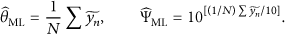
the maximum likelihood estimators of θ and Ψ are, respectively,

$$\begin{array}{cc}& {\widehat{\theta }}_{\text{ML}}=\frac{1}{N}{\displaystyle \sum }‍\widetilde{y_n},\hspace{1em}\hspace{1em}{\widehat{\Psi }}_{\text{ML}}=10^{\left[(1/N)\sum ‍\widetilde{y_n}/10\right]}.\end{array}$$

(24)

If a new target is initialized in multiple targets with unknown reference power, the solution needs to be slightly modified. We have the measurement equation as

$$\begin{array}{cc}& y_n=10\hspace{0.17em}{\log }_{\mathrm{10}}\left(\frac{\Psi }{{{\rm Y}}^2}+{\mathit{\Gamma }}_n\right)+v_n,\end{array}$$

(25)

where ${\mathbf{\Gamma }}_n$ is the predicted measurement part of current targets being tracked. Similarly to the case of a single target initialization, we estimate the squared distances as

$$\begin{array}{cc}& {\left|{\mathit{r}}_n-\mathit{l}\right|}^2\triangleq {{\rm Y}}_n^2=\Psi {\left(10^{y_n/10}-{\mathit{\Gamma }}_n\right)}^{-1}.\end{array}$$

(26)

After canceling out the power,

$$\begin{array}{cc}& \left|\frac{{{\rm Y}}_i}{{{\rm Y}}_j}\right|\triangleq {\gamma }_{ij}=\sqrt{\frac{10^{\left(y_j/10-{\mathit{\Gamma }}_j\right)}}{10^{\left(y_i/10-{\mathit{\Gamma }}_i\right)}}}.\end{array}$$

(27)

The rest of the steps are the same as in the initialization with known reference power, and only ${\gamma }_{ij}$ is differently formulated. In multiple targets case, we cannot apply the ML method directly for estimating the reference power of the new target because we cannot solve the ML function directly in this case due to the ${\mathbf{\Gamma }}_n$ factor, and the maximum log-likelihood function has the formula as follows:

$$\begin{array}{cc}& 10^{\sum y_n/10}={\displaystyle \prod }‍\left(\frac{\Psi }{{{\rm Y}}^2}+{\mathit{\Gamma }}_n\right).\end{array}$$

(28)

Therefore, we apply the LS method one more time for estimating the power of the new target in this case.

5. Particle Filtering as the Solution to Tracking System

The initialization algorithm is only a part of whole tracking system by particle filtering. When the reference power of the target is unknown, the generated particle will have one more element in the state vector, and the initialization algorithm will obtain the location and reference power of the new target. When we apply particle filtering, we need to select an appropriate model among all possible models. The model which has the maximum weight sum will be selected according to the predefined varying patterns of the number of targets. Any particle generates the offspring of a new target even if it can be removed after the “model selection” step or resampling step [27]. Therefore, the “initialization step” is applied to every single particle at every time step of the tracking system.

5.1. Sampling Importance Resampling Particle Filter

There are many versions of particle filtering [28–30] and our choice for a tracking system is “sampling importance resampling (SIR)” particle filter. If we denote state function, measurement function, state, measurement, and the weight by ${\mathbf{f}}_t(·)$ , ${\mathbf{h}}_t(·)$ , ${\mathbf{\chi }}_t$ , ${\mathbf{y}}_t$ , and $w_t^i$ (where t is the time step index and i is the particle index), respectively, the importance density, $q({\mathbf{\chi }}_t\hspace{0.17em}|\hspace{0.17em}{\mathbf{\chi }}_{t-\mathrm{1}}^i,{\mathbf{y}}_{\mathrm{1}:t})$ , will turn out to be the prior density, $p({\mathbf{\chi }}_t\hspace{0.17em}|\hspace{0.17em}{\mathbf{\chi }}_{t-\mathrm{1}}^i)$ , and because resampling is executed at every time step, the weight can be computed by $w_t^i\propto p({\mathbf{y}}_t\hspace{0.17em}|\hspace{0.17em}{\mathbf{\chi }}_t^i)$ , which is the likelihood function.

5.2. SIR Particle Filter Combined with Initialization Algorithm

In a multiple and varying number of target-tracking system, the state space equation must include the state of the number of targets. We denote it by ${\mathbf{K}}_t$ at the time step t. ${\mathbf{K}}_t$ has three patterns to propagate as the previous assumption; that is,

$$\begin{array}{cc}& {\mathit{K}}_t={\mathit{K}}_{t-1}+1,\hspace{1em}\hspace{1em}{\mathit{K}}_t={\mathit{K}}_{t-1},\hspace{1em}\hspace{1em}{\mathit{K}}_t={\mathit{K}}_{t-1}-1.\end{array}$$

(29)

We propagate equal number of particles for each model. The number of targets follows the model for the next time step. Therefore, every single particle will produce multiple descendants depending on the number of possible models. The number of models at the next time step depends on ${\mathbf{K}}_{t-\mathrm{1}}$ . For instance, if ${\mathbf{K}}_{t-\mathrm{1}}=\mathrm{0}$ , then the possible models will be either $\mathrm{0}$ or $\mathrm{1}$ . If ${\mathbf{K}}_{t-\mathrm{1}}=n>\mathrm{0}$ , then the possible ${\mathbf{K}}_t=n-\mathrm{1}$ , n, and $n+\mathrm{1}$ . However, when $n>\mathrm{1}$ , it will have $C_n^{n-\mathrm{1}}$ more multiple models because n targets have equal possibility of disappearance. When ${\mathbf{K}}_t=\mathrm{0}$ , the state space will be empty except for the number of targets. The posterior function of interest will be $p({\mathbf{K}}_{\mathrm{1}:t},{\mathcal{S}}_{\mathrm{1}:t},{\mathbf{x}}_{\mathrm{1}:t}\hspace{0.17em}|\hspace{0.17em}{\mathbf{y}}_{\mathrm{1}:t})$ (where $\mathcal{S}$ is the reference power of the target and x is the state vector), and the distribution is approximated by the “random measure”; that is,

$$\begin{array}{cc}& p\left({\left\{{\mathit{\chi }}_{1:t}\right\}}_{m=1}^M\right)=p\left({\left\{{\mathit{K}}_{1:t}^m,{\mathit{x}}_{1:t}^m,{\mathcal{S}}_{1:t}^m\right\}}_{m=1}^M\right)={\left\{w_{1:t}^m\right\}}_{m=1}^M,\end{array}$$

(30)

where M is the total number of the particles. We can compute the weight when we use SIR particle filter; that is,

$$\begin{array}{cc}& w_t^m\propto p\left(y_{1:N,t}\hspace{0.17em}|\hspace{0.17em}{\mathit{x}}_t^m,{\mathit{K}}_t^m,{\mathcal{S}}_t^m\right).\end{array}$$

(31)

If we use only the three best sensors and assuming that sensors are not correlated, then

$$\begin{array}{cc}& w_t^m\propto {\displaystyle \prod }_{n=1}^{3}p(y_{n,t}\hspace{0.17em}|\hspace{0.17em}{\mathit{x}}_t^m,{\mathit{K}}_t^m,{\mathcal{S}}_t^m).\end{array}$$

(32)

We need to apply the initialization algorithm when we generate a particle that has a newly appearing target (the algorithm generates the estimated location and reference power): this is the case when ${\mathbf{K}}_t^m={\mathbf{K}}_{t-\mathrm{1}}^m+\mathrm{1}$ . In Algorithm 2, we described how to apply initialization, combined with particle filtering. In Algorithm 2, we apply the initialization algorithm that is explained in Section 4 for estimating the distance between each sensor and the new target ( ${{\rm Y}}_{n,t}$ ) and the reference power of the new target. If we cancel out the reference power, we do not use neighboring sensors anymore as shown in Algorithm 2. Note that when the reference power is known, the initialization algorithm has to use the sensors that are neighboring to each other (see Algorithm 1).

Algorithm 2 (tracking multitargets by particle filtering and linear least squares method at an arbitrary time step).

At time t, from the all measurements $y_{s_{\mathrm{1}:N}}$ , find the four best measurements ( $y_{(s_{\mathrm{1}},s_{\mathrm{2}},s_{\mathrm{3}},s_{\mathrm{4}}),t}$ ) and corresponding sensors' identities ( $s_{\mathrm{1}},s_{\mathrm{2}},s_{\mathrm{3}},s_{\mathrm{4}}$ ). Suppose ${\mathbf{K}}_{t-\mathrm{1}}^m=\mathrm{1}$ , and it can be easily generalized for any value of ${\mathbf{K}}_{t-\mathrm{1}}^m$ .

• (i)

$\eta =\mathrm{0}$ , where η is an auxiliary index.

(ii)

For   $m=1:M$ (M is the number of particles.)

• (a)

Model 1: ${\mathbf{K}}_t^{M+\mathrm{1}+\eta }=\mathrm{0}$ (particle $M+\mathrm{1}+\eta$ is generated from particle m). The elements of the other states become empty. Compute the weight, $w_t^{M+\mathrm{1}+\eta }$ .

(b)

Model 2: ${\mathbf{K}}_t^m=\mathrm{1}$ (particle m is generated from particle m). Generate a new particle ${\mathbf{\chi }}_t^m$ as follows: ${\mathbf{\chi }}_t^m=\{{\mathbf{K}}_t^m,{\mathcal{S}}_t^m,{\mathbf{x}}_t^m\}=\{\mathrm{1},{\mathcal{S}}_t^m,{\mathbf{x}}_t^m\}$ , $\left\{{\mathbf{x}}_t^m,{\mathcal{S}}_t^m\right\}~p({\mathbf{x}}_t,{\mathcal{S}}_t\hspace{0.17em}|\hspace{0.17em}{\mathbf{x}}_{t-\mathrm{1}}^m,{\mathcal{S}}_{t-\mathrm{1}}^m)$ according to SIR particle filter. Compute the weight, $w_t^m$ .

(c)

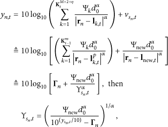
Model 3: ${\mathbf{K}}_t^{M+\mathrm{2}+\eta }=\mathrm{2}$ (particle $M+\mathrm{2}+\eta$ is generated from particle m). We suppose

$$\begin{array}{cc}& y_{n,t}=10\hspace{0.17em}{\log }_{\mathrm{10}}\left({\displaystyle \sum }_{k=1}^{{\mathit{K}}_t^{M+2+\eta }}\frac{{\Psi }_k{d}_0^{\alpha }}{{\left|{\mathit{r}}_n-{\mathit{l}}_{k,t}\right|}^{\alpha }}\right)+v_{s_n,t}\\ \triangleq 10\hspace{0.17em}{\log }_{\mathrm{10}}\left[\left({\displaystyle \sum }_{k=1}^{{\mathit{K}}_{t-1}^m}\frac{{\Psi }_k{d}_0^{\alpha }}{{\left|{\mathit{r}}_n-{\mathit{l}}_{k,t}^p\right|}^{\alpha }}\right)+\frac{{\Psi }_{\text{new}}{d}_0^{\alpha }}{{\left|{\mathit{r}}_n-{\mathit{l}}_{\text{new},t}\right|}^{\alpha }}\right]\\ \triangleq 10\hspace{0.17em}{\log }_{\mathrm{10}}\left[{\mathit{\Gamma }}_n+\frac{{\Psi }_{\text{new}}{d}_0^{\alpha }}{{{\rm Y}}_{s_n,t}^{\alpha }}\right],\hspace{0.17em}\hspace{0.17em}\text{then}\\ \hspace{0.17em}{{\rm Y}}_{s_n,t}={\left(\frac{{\Psi }_{\text{new}}{d}_0^{\alpha }}{10^{\left(y_{s_n,t}/10\right)}-{\mathit{\Gamma }}_n}\right)}^{1/\alpha },\end{array}$$

(33)

 

where ${\mathbf{\Gamma }}_n={\sum }_{k=\mathrm{1}}^{{\mathbf{K}}_{t-\mathrm{1}}^m}‍({\Psi }_k{d}_{\mathrm{0}}^{\alpha }/|{\mathbf{r}}_n-{\mathbf{l}}_{k,t}^p{|}^{\alpha })$ which is predicted part of measurements for the continuing targets, ${{\rm Y}}_{s_n,t}=|{\mathbf{r}}_n-{\mathbf{l}}_{\text{new},t}|$ which is the estimated distance between the new target and each sensor, ${\Psi }_{\text{new}}$ is the reference power of the new target, and ${\mathbf{l}}_{k,t}^p$ is the predicted location of targets propagating from the previous time step, which is propagated from the previous particle.

• (1)

From ${{\rm Y}}_{s_{\mathrm{1}:\mathrm{4}},t}$ , power is canceled out as follows (if α is 2):

$$\begin{array}{cc}& \left|\frac{{{\rm Y}}_{s_i}}{{{\rm Y}}_{s_j}}\right|\triangleq {\gamma }_{ij}=\sqrt{\frac{10^{\left(y_j/10-{\mathit{\Gamma }}_j\right)}}{10^{\left(y_i/10-{\mathit{\Gamma }}_i\right)}}},\hspace{1em}i=1,\hspace{0.17em}\hspace{0.17em}j=\mathrm{2,3},4.\end{array}$$

(34)

(2)

The LS method is applied to estimate ${\mathbf{l}}_{\text{new}}$ , and then estimate the reference power given ${\mathbf{l}}_{\text{new}}$ .

(3)

Compute the weight, $w_t^{M+\mathrm{2}+\eta }$ .

(d)

$\eta =\eta +\mathrm{2}$ , where η increases by 2 because we have three patterns.

 

end

(iii)

Compute weight sum of each model to select the maximum, and then estimate the state in minimum mean squared error criterion.

6. Computer Simulations

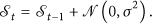
In this section, we present computer simulations based on the proposed approach. The validity of the proposed algorithm is verified by using MATLAB version $\mathrm{7.12.0}.\mathrm{635}$ (R $\mathrm{2011}$ a). All simulations were performed by m-files coded by the authors. We apply the algorithm shown in Algorithm 2 at every time step for the whole tracking system. We assume that the reference power of the target is unknown and varies as

$$\begin{array}{cc}& {\mathcal{S}}_t={\mathcal{S}}_{t-1}+\mathcal{N}(0,{\sigma }^2).\end{array}$$

(35)

The initial reference power is given by $\mathrm{200}$ and $\mathrm{180}$  (J/s) to each target. The number of particles is $\mathrm{300}$ when we apply particle filtering. A target appears at the coordination of (0,150) initially, and, two time steps later, another target appears at the coordination of (200,0) and both targets remain together until the time step is $\mathrm{62}$ . From the time step $\mathrm{63}$ , the second target disappears and only first target lasts until the time step $\mathrm{80}$ . Acceleration-noise follows zero mean Gaussian distribution with variance $\mathrm{1}$ , background noise power is $\mathrm{0.01}$  (dB), the variance of the reference power is $\mathrm{0.001}$ , and the number of sensors is $\mathrm{5}$ -by-5 = 25. A single simulation result is depicted in Figure 8. We ran $\mathrm{1000}$ simulations of the scenario that generates the result of Figure 8. The results show that generally the algorithm performs well with accurate detection of a new target and disappearance of the target. When we initialize a new target, the target which has unduly low reference power and the target that is located out of the field of interest are removed even if it is initialized as a new target. Figures 9(a)-9(b) show the results of mean error for each coordinate, and Figures 9(c)-9(d) show the results of $\mathrm{1000}$ runs comparing true power and the mean of estimated power for each target. Note that the error increases during the time steps from $\mathrm{3}$ to $\mathrm{62}$ for target $\mathrm{1}$ as shown in Figures 9(a)-9(b). The result is shown in Table 2.

Table 2

Mean error of the initialized parameters.

	X-coordinate	Y-coordinate	Reference power
Target 1	−0.0465	0.2536	−0.0936
Target 2	0.5690	0.5060	0.0327

Figure 8

Tracking two targets in 2D sensor filed.

Figure 9

The simulation result by $\mathrm{1000}$ runs. Power estimate is mean of $\mathrm{1000}$ runs.

7. Summary and Conclusions

In this paper, we proposed a general multi-target-tracking algorithm by particle filtering based on the RSS measurement model where multiple targets are unidentified, the number of targets varies, and also unknown reference power of the target varies. We introduced the initialization step in the tracking algorithm where the LS and ML methods are applied as the substeps. The proposed approach can be applied to very crucial practical problems such as tracking mobile phone users or wearable devices in a wireless cellular system or tracking moving sensor nodes in ad hoc wireless sensor networks even though generally the reference power is known in these practical problems. This approach also can be applied for ubiquitous 3D positioning system in emerging visible-light communications systems based on light-emitting diodes. The proposed approach assumes generally a number of parameters are unknown, that is, the number of targets, the reference power of the target, and the initial location of the target, which provides possibilities of using the proposed approach in highly challenging environment.