Distributed Box Particle Filtering for Target Tracking in Sensor Networks

Abstract

Distributed target tracking is a significant technique and is widely used in many applications. Combined with the interval analysis, box particle filtering (BPF) has been proposed to solve the problem of Bayesian filtering when the uncertainties in the measurements are intervals; that is, the measurements are interval-based vectors. This paper is targeted for extending the existing BPF based on a single sensor to a distributed sensor network. We propose a distributed BPF (d-BPF) that each sensor communicates with its direct neighbors to collaboratively estimate the states of the target. The feasibility of the proposed distributed BPF is justified, and some numerical simulations are presented to show its effectiveness in target tracking.

1. Introduction

Target tracking is a prevalent task in many scenarios, such as navigation, military, and transportation. In the literature, various approaches have been proposed for target tracking [1, 2]. One of the most popular approaches is the Bayesian inference [3]. Within the Bayesian framework, the posterior probability density function (pdf) of the states of the target is calculated, conditioned on the available measurements obtained by sensors. Then, based on the obtained posterior pdf, the states of the target can be estimated, correspondingly.

Reviewing the related works of target tracking based on Bayesian inference, the Kalman filter (KF) [4–6] is a classical approach. However, in the presence of the nonlinearities and non-Gaussian uncertainties, the KF becomes inefficient. To tackle this problem, extended trackers such as the extended Kalman filter (EKF) [7] and the unscented Kalman filter (UKF) [8] have been developed. Although these extended trackers can handle some nonlinear cases, they become ineffective when the high-variance measurements and state noise combined with nonlinearities exist [9]. The particle filter (PF), which represents the posterior pdf of the states by sampling, shows outstanding performance, especially for nonlinear and/or non-Gaussian cases [3]. However, the efficiency and accuracy of the PF largely depend on the number of the particles. In the case where a large number of particles are used, the computational complexity is quite high.

It is worth pointing out that all of the above-mentioned approaches can only deal with the point measurements represented by fixed vectors. However, for a large amount of target tracking problems, the uncertainties may lie in a certain region, and thus the measurements are intervals. To deal with such interval-based uncertainties, the box particle filtering (BPF) [10–12] based on the interval framework is proposed, which propagates a set of weighted boxes in a sequential way. Instead of using a large amount of point samples, much less weighted boxes are used to approximate the desired moments of the posterior pdfs.

On the other hand, distributed in-network target tracking, where a set of distributed sensors collaboratively estimate the states of target, has received much attention recently. Distributed tracking can achieve low energy consumption as well as high robustness and scalability. Owing to these merits, various distributed target tracking algorithms have been proposed, such as the distributed KF [13–15] and the distributed PF [16–19].

However, the above-distributed algorithms are only used for the cases where the system measurements are point-based vectors. Decentralized BPF that can handle interval-based uncertainties has not aroused much attention. Although a decentralized BPF algorithm using belief propagation (BP) like message-passing algorithm is proposed in [20], it is only focused on the context of target localization but not applied to target tracking. Considering this, a distributed BPF (d-BPF) algorithm is proposed in this paper, where only the one-hop data exchange and communication between sensors and their neighbors are used to collaboratively track the states of the target. Theoretical studies and numerical simulations are then performed to show the effectiveness of the proposed algorithm.

The rest of this paper is organized as follows. In Section 2, we review some basic knowledge related to BPF. In Section 3, we derive the d-BPF and analyze the feasibility of the d-BPF. The selection of the combination weights for cooperation is also introduced in the same section. Section 4 presents some simulation examples. Finally, some conclusion is drawn in Section 5.

2. Preliminaries

The traditional Bayesian estimation deals with the point measurements, while the BPF can cope with interval-based measurements. The key idea of the BPF is to replace a particle by a multidimensional interval in the state space [11]. Therefore, the derivation of BPF depends on the theory of interval framework. So, before introducing the BPF, we overview some basic knowledge of interval analysis, including interval arithmetic and inclusion function, as well as constraint satisfaction problems and contraction.

2.1. Interval arithmetic

A real interval $[x]$ is a nonempty set of real numbers:

$$\begin{array}{cc}& \left[x\right]=\left[\underset{\_}{x},\bar{x}\right]=\left\{x\in \mathbb{R}\hspace{0.17em}|\hspace{0.17em}\underset{\_}{x}\le x\le \bar{x}\right\},\end{array}$$

(1)

where $\underset{\_}{x}$ and $\bar{x}$ denote the lower and upper bounds of $[x]$ , respectively. From this definition, it is natural to define set-theoretic operations, such as intersection and union, and the results of these must be intervals also. For instance, the interval union of two intervals $[x]\bigsqcup [y]$ is defined as

$$\begin{array}{cc}& \left[x\right]{\displaystyle \bigsqcup }\left[y\right]=\left[\left[x\right]\cup \left[y\right]\right],\end{array}$$

(2)

where the symbol “∪” denotes the union on sets and the symbol “ $[·]$ ” denotes the interval hull operator returning the smallest interval enclosing S, for any set S in real set $\mathbb{R}$ [25].

The interval intersection of two intervals $[x]\sqcap [y]$ is defined as

$$\begin{array}{cc}& \left[x\right]\sqcap \left[y\right]=\left[x\right]\cap \left[y\right],\end{array}$$

(3)

where the symbol “∩” denotes the intersection on sets.

Interval arithmetic operations are also defined on $\mathbb{I}\mathbb{R}$ such that the interval result encloses all possible real results, where $\mathbb{I}\mathbb{R}$ denotes a set of all real-valued intervals. Given $[x]=[\underset{\_}{x},\bar{x}]$ and $[y]=[\underset{\_}{y},\bar{y}]$ , the binary operations $\{+,-,\times ,/\}$ can be defined by

$$\begin{array}{cc}& \left[z\right]=\left[x\right]\otimes \left[y\right]=\left[\left\{x\otimes y\hspace{0.17em}|\hspace{0.17em}x\in \left[x\right],\hspace{0.17em}\hspace{0.17em}y\in \left[y\right]\right\}\right],\end{array}$$

(4)

where ⊗ denotes the binary operations.

Some basic interval arithmetic operations are summarized in Table 1 [25]. An interval vector $[\mathbf{x}]$ is defined as a vector with interval components and the space of all $n_x$ dimension interval vectors is denoted by

$$\begin{array}{cc}& \left[\mathbf{x}\right]=\left[x_{\mathrm{1}}\right]\times \left[x_{\mathrm{2}}\right]\times \cdots \times \left[x_{n_x}\right].\end{array}$$

(5)

Table 1

Interval arithmetic operations.

Binary operator	Notation
$$[x]+[y]$$	$$[\underset{\_}{x}+\underset{\_}{y},\bar{x}+\bar{y}]$$
$$[x]-[y]$$	$$[\underset{\_}{x}-\bar{y},\bar{x}-\underset{\_}{y}]$$
$$[x]\times [y]$$	$$[\min (\underset{\_}{x}\underset{\_}{y},\underset{\_}{x}\bar{y},\bar{x}\underset{\_}{y},\bar{x}\bar{y}),\max (\underset{\_}{x}\underset{\_}{y},\underset{\_}{x}\bar{y},\bar{x}\underset{\_}{y},\bar{x}\bar{y})]$$
$$[x]/[y]$$	$$[x]\times [\mathrm{1}/\underset{\_}{y},\mathrm{1}/\bar{y}]$$ , if $$\mathrm{0}\notin [y]$$
	$$[\bar{x}/\underset{\_}{y},\mathrm{\infty }]$$ , if $$\bar{x}\le \mathrm{0}$$ and $$\bar{y}=\mathrm{0}$$
	$$[-\mathrm{\infty },\bar{x}/\bar{y}]\cup [\bar{x}/\underset{\_}{y},\mathrm{\infty }]$$ , if $$\bar{x}\le \mathrm{0}$$ and $$\underset{\_}{y}<\mathrm{0}<\bar{y}$$
	$$[-\mathrm{\infty },\bar{x}/\bar{y}]$$ , if $$\bar{x}\le \mathrm{0}$$ and $$\underset{\_}{y}=\mathrm{0}$$
	$$[-\mathrm{\infty },\mathrm{\infty }]$$ , if $$\underset{\_}{x}<\mathrm{0}<\bar{x}$$
	$$[-\mathrm{\infty },\underset{\_}{x}/\underset{\_}{y}]$$ , if $$\underset{\_}{x}\ge \mathrm{0}$$ and $$\bar{y}=\mathrm{0}$$
	$$[-\mathrm{\infty },\underset{\_}{x}/\underset{\_}{y}]\cup [\underset{\_}{x}/\bar{y},\mathrm{\infty }]$$ , if $$\underset{\_}{x}\ge \mathrm{0}$$ and $$\underset{\_}{y}<\mathrm{0}<\bar{y}$$
	$$[\underset{\_}{x}/\bar{y},\mathrm{\infty }]$$ , if $$\underset{\_}{x}\ge \mathrm{0}$$ and $$\underset{\_}{y}=\mathrm{0}$$

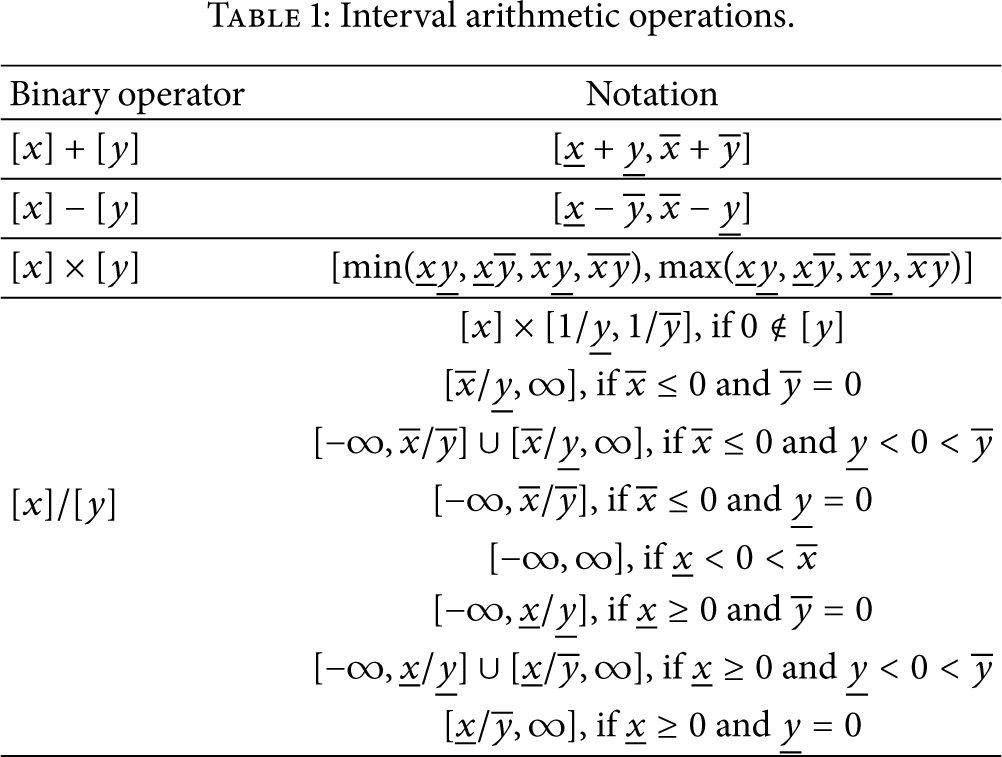
Similarly, interval arithmetic to boxes can be extended straightforwardly [25].

2.2. Inclusion Function

As mentioned above, in the BPF, each particle is replaced by a multidimensional interval in the state space. In order to keep consistency, it is necessary to guarantee that the result of interval operation is still an interval or an interval vector. Fortunately, an inclusion function can meet our need. To make it simple, assume f is a function from ${\mathbb{R}}^{n_x}$ to ${\mathbb{R}}^m$ . In the BPF, when propagating box particles via the continuous nonlinear function f, the mapping of the box particle is not necessary a box. But it can be approximated by an inclusion function. An interval function $[\mathbf{f}]$ from $\mathbb{I}{\mathbb{R}}^{n_x}$ to $\mathbb{I}{\mathbb{R}}^m$ is said to be an inclusion function for f if

$$\begin{array}{cc}& \mathbf{f}\left(\left[\mathbf{x}\right]\right)\subseteq \left[\mathbf{f}\right]\left(\left[\mathbf{x}\right]\right),\forall \left[\mathbf{x}\right]\in \mathbb{I}{\mathbb{R}}^{n_x}.\end{array}$$

(6)

An inclusion function may be very pessimistic. But the minimal inclusion function for f denoted by $[\mathbf{f}{]}^{\ast }$ is unique [11].

2.3. Constraint Satisfaction Problems and Contraction Methods

Consider variables $x_i$ in $\mathbb{R}$ , $i\in \{\mathrm{1},\dots ,n_x\}$ , linked by m relations (or constraints) of the form

$$\begin{array}{cc}& f_j\left(x_{\mathrm{1}},\dots ,x_{n_x}\right)=\mathrm{0},j=\mathrm{1},\dots ,m.\end{array}$$

(7)

Define the vector x as $\mathbf{x}=(x_{\mathrm{1}},\dots ,x_{n_x}{)}^T$ , where T denotes transposition, and let f is a vector function whose components are $f_j$ , $j=\mathrm{1},\dots ,m$ . Then, the m constraints can be rewritten as

$$\begin{array}{cc}& \mathbf{f}\left(\mathbf{x}\right)=\mathbf{0}.\end{array}$$

(8)

This corresponds to a constraint satisfaction problem (CSP), which is denoted as $\mathcal{H}$ ; that is,

$$\begin{array}{cc}& \mathcal{H}:\left(\mathbf{f}\left(\mathbf{x}\right)=\mathbf{0},\hspace{0.17em}\hspace{0.17em}\mathbf{x}\in \left[\mathbf{x}\right]\right),\end{array}$$

(9)

and the solution set of $\mathcal{H}$ is defined as

$$\begin{array}{cc}& \mathbb{S}=\left\{\mathbf{x}\in \left[\mathbf{x}\right]\hspace{0.17em}|\hspace{0.17em}\mathbf{f}\left(\mathbf{x}\right)=\mathbf{0}\right\}.\end{array}$$

(10)

Note that the set $\mathbb{S}$ is not necessary a box. Within the interval framework, the term contracting refers to solving a CSP, that is, finding the smallest box ${\left[\mathbf{x}\right]}^{\prime }\subset [\mathbf{x}]$ that constitutes an outer approximation of $\mathbb{S}$ such that $\mathbb{S}\subseteq {\left[\mathbf{x}\right]}^{\prime }\subseteq [\mathbf{x}]$ . In the BPF, a general and well-known contraction method, the constraints propagation (CP) technique is applied [12]. Illustrative examples of CP method can be found in [11].

3. Target Tracking with Distributed Box Particle Filtering

Assume that there are N static sensors and a moving target. These sensors are randomly distributed over a geometrical field with known positions and can periodically obtain measurements from the target. Our goal is to track the target in a distributed way so as to improve the tracking accuracy. We firstly derive the d-BPF algorithm and then give the Bayesian justification for it. Finally, some choices for the combination weight are given.

3.1. Distributed Box Particle Filtering

Consider the following state-space model:

$$\begin{array}{cc}& {\mathbf{x}}_{t+\mathrm{1}}=\mathbf{f}\left({\mathbf{x}}_t,{\mathbf{v}}_{t+\mathrm{1}}\right),\\ {\mathbf{y}}_{k,t+\mathrm{1}}={\mathbf{g}}_k\left({\mathbf{x}}_{t+\mathrm{1}}\right)+{\mathbf{w}}_{k,t+\mathrm{1}},k=\mathrm{1},\dots ,N,\end{array}$$

(11)

where $\mathbf{f}:{\mathbb{R}}^{n_x}\to {\mathbb{R}}^{n_x}$ is a nonlinear transition function from time t to $t+\mathrm{1}$ with $n_x$ being the dimension of the states. ${\mathbf{v}}_{t+\mathrm{1}}$ denotes an independent identically distributed (i.i.d.) process noise. Function ${\mathbf{g}}_k:{\mathbb{R}}^{n_x}\to {\mathbb{R}}^{n_y}$ defines the relationship between the states and the measurements in node k at time $t+\mathrm{1}$ , where $n_y$ is the dimension of the measurements. ${\mathbf{w}}_{k,t+\mathrm{1}}$ is an i.i.d. measurement noise of node k. Here, we consider interval-based uncertainties and thus interval measurements. That is, each sensor k provides interval measurements $[{\mathbf{y}}_{k,t+\mathrm{1}}]$ , which can be expressed as $[{\mathbf{y}}_{k,t+\mathrm{1}}]=[{\mathbf{y}}_{k,t+\mathrm{1}}+{\Delta }_{\mathrm{1}},{\mathbf{y}}_{k,t+\mathrm{1}}+{\Delta }_{\mathrm{2}}]$ , where ${\Delta }_{\mathrm{1}}$ and ${\Delta }_{\mathrm{2}}$ denote the lower bound and the higher bound uncertainties, respectively. It is assumed that each node knows the locations of its neighbors at each time t.

In [10, 11], target tracking with a single sensor using BPF algorithm has been studied. Different from the PF, in the BPF, each particle is a box, which takes into account the imprecision caused by the model errors [11]. In this manner, the contraction step is similar to the variance matrix measurement update step of the Kalman filtering. Therefore, we follow a similar guideline of distributed Kalman filtering [26] to derive a distributed BPF algorithm for target tracking in a sensor network.

The d-BPF algorithm can be divided into five steps: initialization, time update and measurements broadcast, measurement update, estimation fusion, and resampling, where the second to the fourth steps are shown schematically in Figure 1.

Figure 1

The schematic process of the d-BPF algorithm.

(i) Initialization. At the beginning, the box particles in each node have to be initialized. Taking node k as an example, it can be initialized by M equally weighted and mutually disjoint boxes represented by $\{[{\mathbf{x}}_{k,\mathrm{0}}^{(m)}],{\omega }_{k,\mathrm{0}}^{(m)}{\}}_{m=\mathrm{1}}^M$ , where $[{\mathbf{x}}_{k,\mathrm{0}}^{(m)}]$ denotes the box particles and ${\omega }_{k,\mathrm{0}}^{(m)}$ denotes the corresponding weights. The BPF is superior to the PF in that it can cover larger prior uncertainty region with much fewer box particles.

(ii) Time Update and Measurements Broadcast. Referring to Figure 1(a), each node obtains a set of predicted box particles according to the transition function locally and broadcasts measurements to its close neighbors simultaneously. Knowing a set of weighted box particles $\{[{\mathbf{x}}_{k,t}^{(m)}],{\omega }_{k,t}^{(m)}{\}}_{m=\mathrm{1}}^M$ at time step t and assuming that the system noise is known to be enclosed in the interval $[{\mathbf{v}}_{t+\mathrm{1}}]$ , the predicted boxes at step $t+\mathrm{1}$ can be calculated by

$$\begin{array}{cc}& \left[{\mathbf{x}}_{k,t+\mathrm{1}}^{\left(m\right)}\right]=\left[\mathbf{f}\right]\left(\left[{\mathbf{x}}_{k,t}^{\left(m\right)}\right],\left[{\mathbf{v}}_{t+\mathrm{1}}\right]\right),m=\mathrm{1},\dots ,M.\end{array}$$

(12)

It is worth mentioning that the inclusion function $[\mathbf{f}]$ needs to be used for ensuring that the predicted box particle is still an interval when propagating the box particles.

(iii) Measurement Update. As shown in Figure 1(b), after performing time update locally and broadcasting measurements to the neighbors, the weights of the predicted box particles in each node are then updated using the new available measurements from its neighbors (including itself) at time step $t+\mathrm{1}$ . This is an important step in the d-BPF, which is different from the BPF. For all box particles ( $m=\mathrm{1}\cdots M$ ) in node k, we have the predicted box measurements expressed as

$$\begin{array}{cc}& \left[{\mathbf{y}}_{l,t+\mathrm{1}}^{\left(m\right)}\right]=\left[{\mathbf{g}}_l\right]\left(\left[{\mathbf{x}}_{k,t+\mathrm{1}}^{\left(m\right)}\right]\right),\forall l\in {\mathcal{N}}_k,\end{array}$$

(13)

where $[{\mathbf{g}}_l]$ is an inclusion function for ${\mathbf{g}}_l$ and ${\mathcal{N}}_k$ represents the neighbors of node k.

Likelihood factors are calculated using innovation quantities, which reflects the proximity between the measured box and the predicted box measurement [11, 20]. The innovation is represented by the intersection between these two boxes, expressed as

$$\begin{array}{cc}& \left[{\mathbf{r}}_{l,t+\mathrm{1}}^{\left(m\right)}\right]=\left[{\mathbf{y}}_{l,t+\mathrm{1}}^{\left(m\right)}\right]\cap \left[{\mathbf{y}}_{l,t+\mathrm{1}}\right],\forall l\in {\mathcal{N}}_k.\end{array}$$

(14)

The likelihood factor is calculated based on the following idea: if predicted measurement of a box particle is included in the new measurement box, its updated weight should be larger. In contrast, if its predicted measurement does not have any intersection with the new measurement box, its updated weight should be equal to zero [11]. Furthermore, the contraction step is used to remove the intervals in the box particles that are not consistent with the measurements. Based on these concepts, for each node k, the likelihood of a box particle at time $t+\mathrm{1}$ can be expressed in the form

$$\begin{array}{cc}& {Ł}_{k,t+\mathrm{1}}^{\left(m\right)}={\displaystyle \prod }_{j=\mathrm{1}}^{n_x}{Ł}_{k,t+\mathrm{1}}^{\left(m\right),j},\end{array}$$

(15)

where

$$\begin{array}{cc}& {Ł}_{k,t+\mathrm{1}}^{\left(m\right),j}=\frac{\left|\left[{\tilde{\mathbf{x}}}_{k,t+\mathrm{1}}^{\left(m\right)}\left(j\right)\right]\right|}{\left|\left[{\mathbf{x}}_{k,t+\mathrm{1}}^{\left(m\right)}\left(j\right)\right]\right|}.\end{array}$$

(16)

Note that the term $[{\tilde{\mathbf{x}}}_{k,t+\mathrm{1}}^{(m)}(j)]$ in (16) represents the jth dimension of updated mth box particle after contraction using all the new available measurements that node k receives. $\left|·\right|$ denotes the length of the interval. The implementation of contraction step is given in Algorithm 1.

Algorithm 1 (contraction in measurement update).

Consider the following.

Input

• (i)

$\{[{\mathbf{x}}_{k,t+\mathrm{1}}^{(m)}],{\omega }_{k,t+\mathrm{1}}^{(m)}{\}}_{m=\mathrm{1}}^M$ : a set of weighted boxes,

(ii)

$[{\mathbf{y}}_{l\in {\mathcal{N}}_k,t+\mathrm{1}}]$ : new available measurements at node k.

( $Nested\hspace{0.17em}\hspace{0.17em}loops$ )

For $l\in {\mathcal{N}}_k$

• (1)

Predicted measurement:

$$\begin{array}{cc}& \left[{\mathbf{y}}_{l,t+\mathrm{1}}^{\left(m\right)}\right]=\left[{\mathbf{g}}_l\right]\left(\left[{\mathbf{x}}_{k,t+\mathrm{1}}^{\left(m\right)}\right]\right),\text{for\hspace{0.17em}\hspace{0.17em}}m=\mathrm{1},\dots ,M.\end{array}$$

(17)

(2)

Innovation:

$$\begin{array}{cc}& \left[{\mathbf{r}}_{l,t+\mathrm{1}}^{\left(m\right)}\right]=\left[{\mathbf{y}}_{l,t+\mathrm{1}}^{\left(m\right)}\right]\cap \left[{\mathbf{y}}_{l,t+\mathrm{1}}\right],\text{for\hspace{0.17em}\hspace{0.17em}}m=\mathrm{1},\dots ,M.\end{array}$$

(18)

(3)

Contraction:

  

If $[{\mathbf{r}}_{l,t+\mathrm{1}}^{(m)}]\ne \varnothing$ , then contract $[{\mathbf{x}}_{k,t+\mathrm{1}}^{(m)}]$ using $[{\mathbf{r}}_{l,t+\mathrm{1}}^{(m)}]$ and CP algorithm to obtain $[{\tilde{\mathbf{x}}}_{k,t+\mathrm{1}}^{(m)}]$ , else $[{\tilde{\mathbf{x}}}_{k,t+\mathrm{1}}^{(m)}]=\varnothing$ , for $m=\mathrm{1},\dots ,M$ .

(4)

Return to step 1, replace $[{\mathbf{x}}_{k,t+\mathrm{1}}^{(m)}]$ by $[{\tilde{\mathbf{x}}}_{k,t+\mathrm{1}}^{(m)}]$ .

Endfor

Output

• (i)

$\{[{\tilde{\mathbf{x}}}_{k,t+\mathrm{1}}^{(m)}],{\omega }_{k,t+\mathrm{1}}^{(m)}{\}}_{m=\mathrm{1}}^M$ : a set of weighted boxes after contraction.

Based on the likelihood in (15), the update weights for each node k at time $t+\mathrm{1}$ can be calculated by

$$\begin{array}{cc}& {\omega }_{k,t+\mathrm{1}}^{\left(m\right)}={Ł}_{k,t+\mathrm{1}}^{\left(m\right)}·{\omega }_{k,t}^{\left(m\right)},\end{array}$$

(19)

and then the weights are normalized by the following:

$$\begin{array}{cc}& {\bar{\omega }}_{k,t+\mathrm{1}}^{\left(m\right)}=\frac{{\omega }_{k,t+\mathrm{1}}^{\left(m\right)}}{{\sum }_{m=\mathrm{1}}^M{\omega }_{k,t+\mathrm{1}}^{\left(m\right)}}.\end{array}$$

(20)

Hence, a set of updated weighted box particles $\{[{\tilde{\mathbf{x}}}_{k,t+\mathrm{1}}^{(m)}],{\bar{\omega }}_{k,t+\mathrm{1}}^{(m)}{\}}_{m=\mathrm{1}}^M$ are obtained. Meanwhile, local estimation in each node can be approximated by the weighted particles as

$$\begin{array}{cc}& {\mathbf{\Phi }}_{k,t+\mathrm{1}}={\displaystyle \sum }_{m=\mathrm{1}}^M{\bar{\omega }}_{k,t+\mathrm{1}}^{\left(m\right)}{\mathbf{c}}_{k,t+\mathrm{1}}^{\left(m\right)},\end{array}$$

(21)

where ${\mathbf{c}}_{k,t+\mathrm{1}}^{(m)}$ is the center of the mth box particle ${\tilde{\mathbf{x}}}_{k,t+\mathrm{1}}^{(m)}$ at time step $t+\mathrm{1}$ in node k.

It is remarked that the box particles in each node are different after contraction, since the new available measurements are different in each node. So, it is improper to transmit weights to the neighbors as that performed in the distributed PF. Instead, here we let nodes only broadcast measurements to their closed neighbors in a distributed way and the box particles at each node are obtained based on the information in its neighborhood.

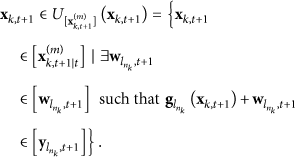
(iv) Estimation Fusion. In Figures 1(c) and 1(d), a combination step is applied and it attempts to achieve the new estimate ${\widehat{\mathbf{x}}}_{k,t+\mathrm{1}}$ that approximates the global performance via local node interactions; that is,

$$\begin{array}{cc}& {\widehat{\mathbf{x}}}_{k,t+\mathrm{1}}={\displaystyle \sum }_{l\in {\mathcal{N}}_k}{a}_{k,l}{\mathbf{\Phi }}_{l,t+\mathrm{1}},\end{array}$$

(22)

where $a_{k,l}$ is the $(k,l)$ element of the combination matrix $A\in {\mathcal{R}}^{N\times N}$ denoting the weight between k and l, which satisfies

$$\begin{array}{cc}& {\mathbb{1}}^{T}A={\mathbb{1}}^T,\\ a_{k,l}=\mathrm{0},\text{if\hspace{0.17em}\hspace{0.17em}}l\notin {\mathcal{N}}_k,\\ a_{k,l}\ge \mathrm{0},\forall k,l,\end{array}$$

(23)

where $\mathbb{1}$ is an $N\times \mathrm{1}$ column vector with unity entries. There are several ways to select $a_{k,l}$ , and this will be described elaborately later.

(v) Resampling. The resampling is performed to introduce variety while preventing the degeneration of the box particles. Similar to the BPF algorithm with a single sensor [10, 11], the multinomial resampling combined with a subdivision step is applied, in which a box particle with high weight is divided by the corresponding number of smaller boxes, instead of obtaining the duplicated particles after the resampling step.

The d-BPF algorithm implements these steps in each time slot and a series of weighted box particles and the state estimation can be calculated sequentially in each node. To summarize, its implementation procedure is given in Algorithm 2.

Algorithm 2 (distributed box particle filtering).

Consider the following.

(1) Initialization. At each node k, set $t=\mathrm{0}$ and generate M box particles $\{[{\mathbf{x}}_{k,\mathrm{0}}^{(m)}],{\omega }_{k,\mathrm{0}}^{(m)}{\}}_{m=\mathrm{1}}^M$ with empty intersection and equal weights.

(2) Time Update and Measurements Broadcast. Assume we have a set of weighted box particles $\{[{\mathbf{x}}_{k,t}^{(m)}],{\omega }_{k,t}^{(m)}{\}}_{m=\mathrm{1}}^M$ in node k at time t.

Calculate the predicted weighted box particles through the transition function in each node locally

$$\begin{array}{cc}& \left[{\mathbf{x}}_{k,t+\mathrm{1}}^{\left(m\right)}\right]=\left[\mathbf{f}\right]\left(\left[{\mathbf{x}}_{k,t}^{\left(m\right)}\right],\left[{\mathbf{v}}_{t+\mathrm{1}}\right]\right),\text{for\hspace{0.17em}\hspace{0.17em}}m=\mathrm{1},\dots ,M.\end{array}$$

(24)

Meanwhile, each node broadcasts measurements to its close neighbors.

(3) Measurement Update

Contraction. Use Algorithm 1 to obtain a set of weighted box particles $\{[{\tilde{\mathbf{x}}}_{k,t+\mathrm{1}}^{(m)}],{\omega }_{k,t+\mathrm{1}}^{(m)}{\}}_{m=\mathrm{1}}^M$ .

Likelihood. Consider

$$\begin{array}{cc}& L_{k,t+\mathrm{1}}^{\left(m\right)}={{\displaystyle \prod }}_{j=\mathrm{1}}^{n_x}{L}_{k,t+\mathrm{1}}^{\left(m\right),j},\text{for\hspace{0.17em}\hspace{0.17em}}m=\mathrm{1},\dots ,M,\end{array}$$

(25)

where

$$\begin{array}{cc}& L_{k,t+\mathrm{1}}^{\left(m\right),j}=\frac{\left|\left[{\tilde{\mathbf{x}}}_{k,t+\mathrm{1}}^{\left(m\right)}\left(j\right)\right]\right|}{\left|\left[{\mathbf{x}}_{k,t+\mathrm{1}}^{\left(m\right)}\left(j\right)\right]\right|}.\end{array}$$

(26)

Weight Update. Consider

$$\begin{array}{cc}& {\omega }_{k,t+\mathrm{1}}^{\left(m\right)}=L_{k,t+\mathrm{1}}^{\left(m\right)}{\omega }_{k,t}^{\left(m\right)},\text{for\hspace{0.17em}\hspace{0.17em}}m=\mathrm{1},\dots ,M.\end{array}$$

(27)

Weight Normalization. Consider

$$\begin{array}{cc}& {\bar{\omega }}_{k,t+\mathrm{1}}^{\left(m\right)}=\frac{{\omega }_{k,t+\mathrm{1}}^{\left(m\right)}}{{\sum }_{m=\mathrm{1}}^M{\omega }_{k,t+\mathrm{1}}^{\left(m\right)}}\text{for\hspace{0.17em}\hspace{0.17em}}m=\mathrm{1},\dots ,M.\end{array}$$

(28)

Local State Estimate. Consider

$$\begin{array}{cc}& {\mathbf{\Phi }}_{k,t+\mathrm{1}}={{\displaystyle \sum }}_{m=\mathrm{1}}^M{\bar{\omega }}_{k,t+\mathrm{1}}^{\left(m\right)}{\mathbf{c}}_{k,t+\mathrm{1}}^{\left(m\right)}.\end{array}$$

(29)

(4) Estimation Fusion. Consider

$$\begin{array}{cc}& {\widehat{\mathbf{x}}}_{k,t+\mathrm{1}}={\displaystyle \sum }_{l\in {\mathcal{N}}_k}{a}_{k,l}{\mathbf{\Phi }}_{l,t+\mathrm{1}}.\end{array}$$

(30)

(5) Resampling. Combine subdivision method for resampling to create M new box particles with the same weights.

(6) Set $t=t+\mathrm{1}$ , and go to step 2 until a predefined number $t^{\mathrm{e}\mathrm{n}\mathrm{d}}$ .

3.2. Distributed Box Particle Filtering Analysis within Bayesian Framework

In this section, similar to the proof of BPF [10, 11], we present the Bayesian justification for d-BPF algorithm. To simplify the representation, we denote the set of all the states and measurements obtained until time t by ${\mathbf{X}}_t=\{{\mathbf{x}}_i,\hspace{0.17em}i=\mathrm{1},\dots ,t\}$ and ${\mathbf{Y}}_t=\{{\mathbf{y}}_i,\hspace{0.17em}i=\mathrm{1},\dots ,t\}$ , respectively. Our objective is to estimate the predicted distribution $p({\mathbf{x}}_{t+\mathrm{1}}\hspace{0.17em}|\hspace{0.17em}{\mathbf{Y}}_t)$ and the posterior distribution $p({\mathbf{x}}_{t+\mathrm{1}}\hspace{0.17em}|\hspace{0.17em}{\mathbf{Y}}_{t+\mathrm{1}})$ , recursively. Once the posterior pdf $p({\mathbf{x}}_{t+\mathrm{1}}\hspace{0.17em}|\hspace{0.17em}{\mathbf{Y}}_{t+\mathrm{1}})$ is estimated, the system states can be calculated, correspondingly.

Within the framework of Bayesian inference, the posterior pdf of the state vector 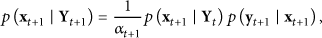$p({\mathbf{x}}_{t+\mathrm{1}}\hspace{0.17em}|\hspace{0.17em}{\mathbf{Y}}_{t+\mathrm{1}})$ is given by

$$\begin{array}{cc}& p\left({\mathbf{x}}_{t+\mathrm{1}}\hspace{0.17em}|\hspace{0.17em}{\mathbf{Y}}_{t+\mathrm{1}}\right)=\frac{\mathrm{1}}{{\alpha }_{t+\mathrm{1}}}p\left({\mathbf{x}}_{t+\mathrm{1}}\hspace{0.17em}|\hspace{0.17em}{\mathbf{Y}}_t\right)p\left({\mathbf{y}}_{t+\mathrm{1}}\hspace{0.17em}|\hspace{0.17em}{\mathbf{x}}_{t+\mathrm{1}}\right),\end{array}$$

(31)

$$\begin{array}{cc}& p\left({\mathbf{x}}_{t+\mathrm{1}}\hspace{0.17em}|\hspace{0.17em}{\mathbf{Y}}_t\right)={{\displaystyle \int }}_{{\mathbb{R}}^{n_x}}p\left({\mathbf{x}}_{t+\mathrm{1}}\hspace{0.17em}|\hspace{0.17em}{\mathbf{x}}_t\right)p\left({\mathbf{x}}_t\hspace{0.17em}|\hspace{0.17em}{\mathbf{Y}}_t\right)d{\mathbf{x}}_t,\end{array}$$

(32)

where ${\alpha }_{t+\mathrm{1}}={\int }_{{\mathbb{R}}^{n_x}}‍p({\mathbf{x}}_{t+\mathrm{1}}\hspace{0.17em}|\hspace{0.17em}{\mathbf{Y}}_t)p({\mathbf{y}}_{t+\mathrm{1}}\hspace{0.17em}|\hspace{0.17em}{\mathbf{x}}_{t+\mathrm{1}})d{\mathbf{x}}_{t+\mathrm{1}}$ is a normalization factor. The recursion can be updated with an initial prior pdf $p({\mathbf{x}}_{\mathrm{0}})$ , for example, a uniform distribution over some region of the state space. Equations (31) and (32) are known as the measurement update and the time update, respectively.

Let a set of box particles be represented by a mixture of uniform pdfs. Comparing with the Gaussian mixture pdf, the uniform pdf is not only simple, but also owns a remarkable adaptation ability to strong nonlinear cases. Based on the interval analysis and by choosing box supports, d-BPF can propagate pdfs through linear, nonlinear, and even differential functions. More specifically, since the particles in the d-BPF algorithm are boxes and with the help of the interval analysis, the box particles can propagate sequentially with the uniform pdf.

Referring to [11], the uniform pdf sum representation of x can be given as

$$\begin{array}{cc}& p\left(\mathbf{x}\right)={\displaystyle \sum }_{m=\mathrm{1}}^M{\omega }^{\left(m\right)}{U}_{\left[{\mathbf{x}}^{\left(m\right)}\right]}\left(\mathbf{x}\right),\\ {\displaystyle \sum }_{m=\mathrm{1}}^M{\omega }^{\left(m\right)}=\mathrm{1},\forall m,{\omega }^{\left(m\right)}\ge \mathrm{0},\end{array}$$

(33)

where $U_{[{\mathbf{x}}^{(m)}]}$ denotes the uniform pdf of the box particle $[{\mathbf{x}}^{(m)}]$ and M denotes the number of mixture components. According to (33), the relative pdfs in the Bayesian inference can be represented by a set of weighted box particles.

Now we can deduce the Bayesian expression of the d-BPF algorithm. Assume that a set of weighted box particles $\{U_{[{\mathbf{x}}_{k,t}^{(m)}]}({\mathbf{x}}_{k,t}),{\omega }_{k,t}^{(m)}{\}}_{m=\mathrm{1}}^M$ of node k is obtained at time t. Consequently, the pdf of the state at time t can be represented by

$$\begin{array}{cc}& p\left({\mathbf{x}}_{k,t}\hspace{0.17em}|\hspace{0.17em}{\mathbf{Y}}_{l\in {\mathcal{N}}_k,t}\right)={\displaystyle \sum }_{m=\mathrm{1}}^M{\omega }_{k,t}^{\left(m\right)}{U}_{\left[{\mathbf{x}}_{k,t}^{\left(m\right)}\right]}\left({\mathbf{x}}_{k,t}\right).\end{array}$$

(34)

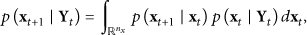
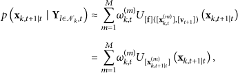
Then, the time update step at each node is carried out locally. Taking node k as an example, according to (32), the pdf of the states can be predicted by

$$\begin{array}{l}p\left({\mathbf{x}}_{k,t+\mathrm{1}\hspace{0.17em}|\hspace{0.17em}t}\hspace{0.17em}|\hspace{0.17em}{\mathbf{Y}}_{l\in {\mathcal{N}}_k,t}\right)\\ ={{\displaystyle \int }}_{{\mathbb{R}}^{n_x}}p\left({\mathbf{x}}_{k,t+\mathrm{1}}\hspace{0.17em}|\hspace{0.17em}{\mathbf{x}}_{k,t}\right)p\left({\mathbf{x}}_{k,t}\hspace{0.17em}|\hspace{0.17em}{\mathbf{Y}}_{l\in {\mathcal{N}}_k,t}\right)d{\mathbf{x}}_{k,t}\\ ={{\displaystyle \int }}_{{\mathbb{R}}^{n_x}}p\left({\mathbf{x}}_{k,t+\mathrm{1}}\hspace{0.17em}|\hspace{0.17em}{\mathbf{x}}_{k,t}\right){\displaystyle \sum }_{m=\mathrm{1}}^M{\omega }_{k,t}^{\left(m\right)}{U}_{\left[{\mathbf{x}}_{k,t}^{\left(m\right)}\right]}\left({\mathbf{x}}_{k,t}\right)d{\mathbf{x}}_{k,t}\\ ={\displaystyle \sum }_{m=\mathrm{1}}^M{\omega }_{k,t}^{\left(m\right)}{{\displaystyle \int }}_{\left[{\mathbf{x}}_{k,t}^{\left(m\right)}\right]}p\left({\mathbf{x}}_{k,t+\mathrm{1}}\hspace{0.17em}|\hspace{0.17em}{\mathbf{x}}_{k,t}\right)U_{\left[{\mathbf{x}}_{k,t}^{\left(m\right)}\right]}\left({\mathbf{x}}_{k,t}\right)d{\mathbf{x}}_{k,t}.\end{array}$$

(35)

Referring to [11], we can derive

$$\begin{array}{l}{{\displaystyle \int }}_{\left[{\mathbf{x}}_{k,t}^{\left(m\right)}\right]}p\left({\mathbf{x}}_{k,t+\mathrm{1}}\hspace{0.17em}|\hspace{0.17em}{\mathbf{x}}_{k,t}\right)U_{\left[{\mathbf{x}}_{k,t}^{\left(m\right)}\right]}\left({\mathbf{x}}_{k,t}\right)d{\mathbf{x}}_{k,t}\\ \approx U_{\left[\mathbf{f}\right]\left(\left[{\mathbf{x}}_{k,t}^{\left(m\right)}\right],\left[{\mathbf{v}}_{t+\mathrm{1}}\right]\right)}\left({\mathbf{x}}_{k,t+\mathrm{1}\hspace{0.17em}|\hspace{0.17em}t}\right).\end{array}$$

(36)

Based on (36), (35) can be rewritten as

$$\begin{array}{l}p\left({\mathbf{x}}_{k,t+\mathrm{1}\hspace{0.17em}|\hspace{0.17em}t}\hspace{0.17em}|\hspace{0.17em}{\mathbf{Y}}_{l\in {\mathcal{N}}_k,t}\right)\approx {\displaystyle \sum }_{m=\mathrm{1}}^M{\omega }_{k,t}^{\left(m\right)}{U}_{\left[\mathbf{f}\right]\left(\left[{\mathbf{x}}_{k,t}^{\left(m\right)}\right],\left[{\mathbf{v}}_{t+\mathrm{1}}\right]\right)}\left({\mathbf{x}}_{k,t+\mathrm{1}\hspace{0.17em}|\hspace{0.17em}t}\right)\\ ={\displaystyle \sum }_{m=\mathrm{1}}^M{\omega }_{k,t}^{\left(m\right)}{U}_{\left[{\mathbf{x}}_{k,t+\mathrm{1}\hspace{0.17em}|\hspace{0.17em}t}^{\left(m\right)}\right]}\left({\mathbf{x}}_{k,t+\mathrm{1}\hspace{0.17em}|\hspace{0.17em}t}\right),\end{array}$$

(37)

where the second equality holds according to (12). So far, we derive that the predicted pdf after time update in each node can still be represented by a set of weighted box particles, where the box particles change according to the transition function, while the weights keep invariant.

In the measurement update step, each node spreads its observations to its neighbors. When nodes receive information from their neighbors, the measurement update step can be implemented. Consequently, according to (31), the posterior pdf of the states can be computed by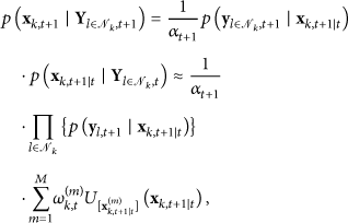

$$\begin{array}{l}p\left({\mathbf{x}}_{k,t+\mathrm{1}}\hspace{0.17em}|\hspace{0.17em}{\mathbf{Y}}_{l\in {\mathcal{N}}_k,t+\mathrm{1}}\right)=\frac{\mathrm{1}}{{\alpha }_{t+\mathrm{1}}}p\left({\mathbf{y}}_{l\in {\mathcal{N}}_k,t+\mathrm{1}}\hspace{0.17em}|\hspace{0.17em}{\mathbf{x}}_{k,t+\mathrm{1}\hspace{0.17em}|\hspace{0.17em}t}\right)\\ ·p\left({\mathbf{x}}_{k,t+\mathrm{1}\hspace{0.17em}|\hspace{0.17em}t}\hspace{0.17em}|\hspace{0.17em}{\mathbf{Y}}_{l\in {\mathcal{N}}_k,t}\right)\approx \frac{\mathrm{1}}{{\alpha }_{t+\mathrm{1}}}\\ ·{\displaystyle \prod }_{l\in {\mathcal{N}}_k}\left\{p\left({\mathbf{y}}_{l,t+\mathrm{1}}\hspace{0.17em}|\hspace{0.17em}{\mathbf{x}}_{k,t+\mathrm{1}\hspace{0.17em}|\hspace{0.17em}t}\right)\right\}\\ ·{\displaystyle \sum }_{m=\mathrm{1}}^M{\omega }_{k,t}^{\left(m\right)}{U}_{\left[{\mathbf{x}}_{k,t+\mathrm{1}\hspace{0.17em}|\hspace{0.17em}t}^{\left(m\right)}\right]}\left({\mathbf{x}}_{k,t+\mathrm{1}\hspace{0.17em}|\hspace{0.17em}t}\right),\end{array}$$

(38)

where ${\alpha }_{t+\mathrm{1}}={\int }_{{\mathbb{R}}^{n_x}}‍p({\mathbf{x}}_{k,t+\mathrm{1}\hspace{0.17em}|\hspace{0.17em}t}\hspace{0.17em}|\hspace{0.17em}{\mathbf{Y}}_{l\in {\mathcal{N}}_k,t})p({\mathbf{y}}_{l\in {\mathcal{N}}_k,t+\mathrm{1}}\hspace{0.17em}|\hspace{0.17em}{\mathbf{x}}_{k,t+\mathrm{1}\hspace{0.17em}|\hspace{0.17em}t})d{\mathbf{x}}_{k,t+\mathrm{1}\hspace{0.17em}|\hspace{0.17em}t}$ is a normalized factor.

Referring to Algorithm 2, the measurement update step consists of two main steps, that is, contraction and weight update. The former is used to contract a set of new box particles and the latter is used to calculate updated weights. Once a set of new weighted box particles is obtained, the estimation can be calculated naturally. We first focus on the contraction step. Since the measurements are intervals, the measurement likelihood function $p({\mathbf{y}}_{l,t+\mathrm{1}}\hspace{0.17em}|\hspace{0.17em}{\mathbf{x}}_{k,t+\mathrm{1}\hspace{0.17em}|\hspace{0.17em}t})$ is taken to be one component with uniform distribution, which is expressed as

$$\begin{array}{cc}& p\left({\mathbf{y}}_{l,t+\mathrm{1}}\hspace{0.17em}|\hspace{0.17em}{\mathbf{x}}_{k,t+\mathrm{1}\hspace{0.17em}|\hspace{0.17em}t}\right)=U_{\left[{\mathbf{y}}_{l,t+\mathrm{1}}\right]}\left({\mathbf{g}}_l\left({\mathbf{x}}_{k,t+\mathrm{1}\hspace{0.17em}|\hspace{0.17em}t}\right)\right).\end{array}$$

(39)

Consequently, (38) can be rewritten as

$$\begin{array}{l}p\left({\mathbf{x}}_{k,t+\mathrm{1}}\hspace{0.17em}|\hspace{0.17em}{\mathbf{Y}}_{l\in {\mathcal{N}}_k,t+\mathrm{1}}\right)=\frac{\mathrm{1}}{{\alpha }_{t+\mathrm{1}}}\\ ·{\displaystyle \prod }_{l\in {\mathcal{N}}_k}\left\{U_{\left[{\mathbf{y}}_{l,t+\mathrm{1}}\right]}\left({\mathbf{g}}_l\left({\mathbf{x}}_{k,t+\mathrm{1}\hspace{0.17em}|\hspace{0.17em}t}\right)\right)\right\}\\ ·{\displaystyle \sum }_{m=\mathrm{1}}^M{\omega }_{k,t}^{\left(m\right)}{U}_{\left[{\mathbf{x}}_{k,t+\mathrm{1}\hspace{0.17em}|\hspace{0.17em}t}^{\left(m\right)}\right]}\left({\mathbf{x}}_{k,t+\mathrm{1}\hspace{0.17em}|\hspace{0.17em}t}\right)=\frac{\mathrm{1}}{{\alpha }_{t+\mathrm{1}}}\\ ·{\displaystyle \sum }_{m=\mathrm{1}}^M\hspace{0.17em}{\displaystyle \prod }_{l\in {\mathcal{N}}_k}\left\{U_{\left[{\mathbf{y}}_{l,t+\mathrm{1}}\right]}\left({\mathbf{g}}_l\left({\mathbf{x}}_{k,t+\mathrm{1}\hspace{0.17em}|\hspace{0.17em}t}^{\left(m\right)}\right)\right)\right\}\\ ·{\omega }_{k,t}^{\left(m\right)}{U}_{\left[{\mathbf{x}}_{k,t+\mathrm{1}\hspace{0.17em}|\hspace{0.17em}t}^{\left(m\right)}\right]}\left({\mathbf{x}}_{k,t+\mathrm{1}\hspace{0.17em}|\hspace{0.17em}t}\right)=\frac{\mathrm{1}}{{\alpha }_{t+\mathrm{1}}}{\displaystyle \sum }_{m=\mathrm{1}}^M{\omega }_{k,t}^{\left(m\right)}\\ ·{\displaystyle \prod }_{l\in {\mathcal{N}}_k}\left\{U_{\left[{\mathbf{y}}_{l,t+\mathrm{1}}\right]}\left({\mathbf{g}}_l\left({\mathbf{x}}_{k,t+\mathrm{1}\hspace{0.17em}|\hspace{0.17em}t}^{\left(m\right)}\right)\right)\right\}{U}_{\left[{\mathbf{x}}_{k,t+\mathrm{1}\hspace{0.17em}|\hspace{0.17em}t}^{\left(m\right)}\right]}\left({\mathbf{x}}_{k,t+\mathrm{1}\hspace{0.17em}|\hspace{0.17em}t}\right).\end{array}$$

(40)

We use $U_{[{\mathbf{y}}_l]}$ to denote $U_{[{\mathbf{y}}_{l,t+\mathrm{1}}]}({\mathbf{g}}_l({\mathbf{x}}_{k,t+\mathrm{1}\hspace{0.17em}|\hspace{0.17em}t}^{(m)}))$ for short. Then, (40) can be rewritten as

$$\begin{array}{l}p\left({\text{X}}_{k,t+1}|{\text{Y}}_{l\in N_k,t+1}\right)=\frac{1}{{\alpha }_{t+1}}\sum _{m=1}^M{\omega }_{k,t}^{(m)}\prod _{l\in N_k}\left\{U_{[\text{y}l]}\right\}\hfill \\ \hspace{0.17em}\hspace{0.17em}\hspace{0.17em}\hspace{0.17em}\cdot U_{[{\text{X}}_{k,t+1|t}^{(m)}]}\left({\text{X}}_{k,t+1|t}\right)=\frac{1}{{\alpha }_{t+1}}\sum _{m=1}^M{\omega }_{k,t}^{(m)}\{U_{[\text{y}{l}_1]}\{U_{[\text{y}{l}_2]}\hfill \\ \hspace{0.17em}\hspace{0.17em}\hspace{0.17em}\dots \left\{U_{[\text{y}{l}_{n_k}]}{U}_{[{\text{X}}_{k,t+1|t}^{(m)}]}\left({\text{X}}_{k,t+1|t}\right)\right\}\}\},\hfill \end{array}$$

(41)

where $l_i\in {\mathcal{N}}_k$ ,   $i=\mathrm{1}\cdots n_k$ with $n_k$ being the degree of node k. The term $U_{[{\mathbf{y}}_{l_{n_k}}]}{U}_{[{\mathbf{x}}_{k,t+\mathrm{1}\hspace{0.17em}|\hspace{0.17em}t}^{(m)}]}({\mathbf{x}}_{k,t+\mathrm{1}\hspace{0.17em}|\hspace{0.17em}t})$ in (41) is a function with a support being the following set:

$$\begin{array}{l}{\text{x}}_{k,t+1}\hspace{0.17em}\in U_{[{\text{X}}_{k,t+1}^{(m)}]}\left({\text{x}}_{k,t+1}\right)=\{{\text{x}}_{k,t+1}\hfill \\ \hspace{0.17em}\hspace{0.17em}\hspace{0.17em}\hspace{0.17em}\in \left[{\text{x}}_{k,t+1|t}^{(m)}\right]|\exists {\text{w}}_{l_{n_k},t+1}\hfill \\ \hspace{0.17em}\hspace{0.17em}\hspace{0.17em}\hspace{0.17em}\in \left[{\text{w}}_{l_{n_k},t+1}\right]\hspace{0.17em}\text{such}\hspace{0.17em}\text{that}\hspace{0.17em}{\text{g}}_{l_{n_k}}\left({\text{x}}_{k,t+1}\right)+{\text{w}}_{l_{n_k},t+1}\hfill \\ \hspace{0.17em}\hspace{0.17em}\hspace{0.17em}\hspace{0.17em}\in \left[{\text{y}}_{l_{n_k},t+1}\right]\}.\hfill \end{array}$$

(42)

Note that the result of $U_{[{\mathbf{y}}_{l_{n_k}}]}{U}_{[{\mathbf{x}}_{k,t+\mathrm{1}\hspace{0.17em}|\hspace{0.17em}t}^{(m)}]}({\mathbf{x}}_{k,t+\mathrm{1}\hspace{0.17em}|\hspace{0.17em}t})$ is also a support, which has the similar expression as $U_{[{\mathbf{x}}^{(m)}]}(\mathbf{x})$ . Repeating this recursively, the result of $\{U_{[{\mathbf{y}}_{{\mathrm{l}}_{\mathrm{1}}}]}\{U_{[{\mathbf{y}}_{l_{\mathrm{2}}}]}\dots \{U_{[{\mathbf{y}}_{l_{n_k}}]}{U}_{[{\mathbf{x}}_{k,t+\mathrm{1}\hspace{0.17em}|\hspace{0.17em}t}^{(m)}]}({\mathbf{x}}_{k,t+\mathrm{1}\hspace{0.17em}|\hspace{0.17em}t})\}\}\}$ is also a support or a box particle. In other words, from (41), it can be seen that the predicted boxes $[{\mathbf{x}}_{k,t+\mathrm{1}\hspace{0.17em}|\hspace{0.17em}t}^{(m)}{]}_{m=\mathrm{1}}^M$ of node k have to be contracted with respect to the new available measurements in node k, including the measurements of its neighbors and itself. By using the contraction step, we obtain a set of new boxes $[{\tilde{\mathbf{x}}}_{k,t+\mathrm{1}}^{(m)}{]}_{m=\mathrm{1}}^M$ for the posterior pdf $p({\mathbf{x}}_{k,t+\mathrm{1}}\hspace{0.17em}|\hspace{0.17em}{\mathbf{Y}}_{l\in {\mathcal{N}}_k,t+\mathrm{1}})$ at time $t+\mathrm{1}$ .

After contraction, the corresponding weights can be calculated according to (16). Finally, the posterior pdf at time $t+\mathrm{1}$ can be expressed as

$$\begin{array}{cc}& p\left({\mathbf{x}}_{k,t+\mathrm{1}}\hspace{0.17em}|\hspace{0.17em}{\mathbf{Y}}_{l\in {\mathcal{N}}_k,t+\mathrm{1}}\right)={\displaystyle \sum }_{m=\mathrm{1}}^M{\bar{\omega }}_{k,t+\mathrm{1}}{U}_{\left[{\tilde{\mathbf{x}}}_{k,t+\mathrm{1}}^{\left(m\right)}\right]}\left({\tilde{\mathbf{x}}}_{k,t+\mathrm{1}}\right),\end{array}$$

(43)

which has the same form as $p({\mathbf{x}}_{k,t}\hspace{0.17em}|\hspace{0.17em}{\mathbf{Y}}_{l\in {\mathcal{N}}_k,t})$ at time t. That is to say, the posterior distribution $p({\mathbf{x}}_{k,t+\mathrm{1}}\hspace{0.17em}|\hspace{0.17em}{\mathbf{Y}}_{l\in {\mathcal{N}}_k,t+\mathrm{1}})$ can be estimated recursively following the framework of Bayesian inference, and thus the feasibility of the d-BPF algorithm is justified.

Remark 3.

It is also remarked that the d-BPF is superior to the noncooperation BPF (Nc-BPF). On the one hand, it can be seen from (42) that the contraction uses the measurements to remove the inconsistent part of each box particle. As a result, combined with measurements of neighbors, the box particles after contraction in each node would have less or at least no more inconsistent part than those without cooperation; that is, the uncertainty of box particle is decreased. On the other hand, according to (16), in the d-BPF algorithm, we can deduce that the box particles with large consistent part have larger normalized weights while those with small consistent part acquire smaller normalized weights, comparing with those in a noncooperation algorithm. As a conclusion, a better set of normalized weights of the box particles can be obtained than that without cooperation and thus the estimate outperforms the noncooperation one.

3.3. Selection of Combination Weight

The entities of combination matrix A represent the weights used to combine the estimates of the neighbors. Some popular choices in the context of graph theory, average consensus, and diffusion adaptive networks are summarized in Table 2, where $d_k$ denotes the degree of node k. In this paper, we employ the metropolis rule as it determines the weights only according to the degrees of the neighbors. According to [23], weights chosen by the metropolis rule can guarantee convergence provided that the graph is not bipartite.

Table 2

Several choices of combination matrix A. In all cases, $$a_{l,k}=\mathrm{0}$$ if $$l\notin {\mathcal{N}}_k$$ , and $$a_{k,k}$$ is chosen such that $${\sum }_{l=\mathrm{1}}^N{a}_{l,k}=\mathit{1}$$ for all k.

Name and reference	Rule $(l\in {\mathcal{N}}_k)$ , $l\ne k$
Uniform [21]	$$a_{l,k}=\mathrm{1}/d_k$$
Laplacian [22, 23]	$$a_{l,k}=\mathrm{1}/d_{\max }$$
Maximum [24]	$$a_{l,k}=\mathrm{1}/N$$
Metropolis [23]	$$a_{l,k}=\mathrm{1}/\max (d_k,d_l)$$

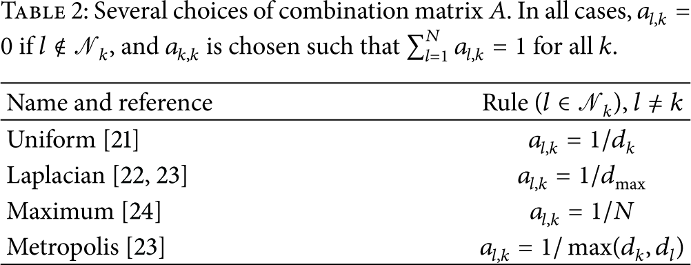
Moreover, considering that the sensors are usually adopted with mobility, a dynamic network topology is also considered. To model this, we assume that the links and nodes are random entities for simplicity. That is, at every time instant t, the undirected random link weight $a_{k,l}(t)=a_{l,k}(t)$ , which connects node k to node l, is set to either a nominal value $a_{k,l}=a_{l,k}$ with probability $p_{k,l}=p_{l,k}$ or zero with probability $q_{k,l}=\mathrm{1}-p_{k,l}$ ; that is, the combination matrix ${\mathbf{A}}_t$ is selected by

$$\begin{array}{cc}& {\left[{\mathbf{A}}_t\right]}_{k,l}=\left\{\begin{array}{cc}{a}_{k,l}\hfill & \text{with probability\hspace{0.17em}\hspace{0.17em}}{p}_{k,l},\hfill \\ \mathrm{0}\hfill & \text{with probability\hspace{0.17em}\hspace{0.17em}}{q}_{k,l}=\mathrm{1}-p_{k,l},\hfill \end{array}\right.\end{array}$$

(44)

where $a_{k,l}$ is selected according to the metropolis rule mentioned above.

Remark 4.

Note that when the sensor network is fully connected, the combination matrix selected by the Metroplis rule becomes $\mathbf{A}=\left(\mathrm{1}/N\right){\mathbf{I}}_N$ , where ${\mathbf{I}}_N$ is an identity $N\times N$ matrix. In this case, the estimate of each node is the same since every node collects the information of all the sensors. That is to say, each sensor can be considered as the fusion center in the centralized processing, and consequently the d-BPF reduces to the centralized BPF (c-BPF).

4. Simulation

In this section, we perform two examples of target tracking using the d-BPF algorithm proposed in Section 3. In these two examples, we consider the target tracking in a 2D plane. Assume there are $N=\mathrm{50}$ sensors randomly deployed in the area of 300 m × 500 m. There is one target in the area and its state information at time t is denoted by ${\mathbf{x}}_t=[x_t,{\dot{x}}_t,y_t,{\dot{y}}_t{]}^T$ , where $x_t$ and $y_t$ represent the position of the target and ${\dot{x}}_t$ and ${\dot{y}}_t$ denote the velocity of the target, respectively. In the following, we will discuss these two examples, respectively.

4.1. Example 1

In the first example, we consider a linear and Gaussian system that can be expressed as

$$\begin{array}{cc}& {\mathbf{x}}_{t+\mathrm{1}}=\mathbf{F}{\mathbf{x}}_t+{\mathbf{v}}_{t+\mathrm{1}}.\end{array}$$

(45)

The target is moving according to the nearly constant velocity model with a transition density function $p({\mathbf{x}}_{t+\mathrm{1}}\hspace{0.17em}|\hspace{0.17em}{\mathbf{x}}_t)=\mathcal{N}({\mathbf{x}}_{t+\mathrm{1}},\mathbf{F}{\mathbf{x}}_t,\mathbf{Q})$ :

$$\begin{array}{cc}& \mathbf{F}={\mathbf{I}}_{\mathrm{2}}\otimes \left(\begin{array}{cc}\mathrm{1}& T\\ \mathrm{0}& \mathrm{1}\end{array}\right),\\ \mathbf{Q}={\mathbf{I}}_{\mathrm{2}}\otimes \left(\begin{array}{cc}\frac{T^{\mathrm{3}}}{\mathrm{3}}& \frac{T^{\mathrm{2}}}{\mathrm{2}}\\ \frac{T^{\mathrm{2}}}{\mathrm{2}}& T\end{array}\right)·\vartheta ,\end{array}$$

(46)

where Q is the covariance matrix of the system noise, ${\mathbf{I}}_{\mathrm{2}}$ is $\mathrm{2}\times \mathrm{2}$ identity matrix, ⊗ is the Kronecker product, T denotes the sampling interval (here set to $\mathrm{1}$ second), and ϑ denotes the process noise intensity (here set to $\mathrm{0.005}$ ). Initially, at $t=\mathrm{0}$ , the target is located at position $(\mathrm{550,300})$  m and is moving with the velocity $(-\mathrm{5},-\mathrm{8.5})$  m/s. The target is tracked for $t=\mathrm{50}$  s.

A nonlinear and Gaussian measurement function g is also used. Each node uses the same measurement model expressed as

$$\begin{array}{cc}& {\mathbf{g}}_k\left({\mathbf{x}}_{t+\mathrm{1}}\right)=\left(\begin{array}{c}{r}_{t+\mathrm{1}}\\ {\dot{r}}_{t+\mathrm{1}}\\ {\theta }_{t+\mathrm{1}}\end{array}\right)=\left(\begin{array}{c}\sqrt{x_{t+\mathrm{1}}^{\mathrm{2}}+y_{t+\mathrm{1}}^{\mathrm{2}}}\\ \frac{x_{t+\mathrm{1}}{\dot{x}}_{t+\mathrm{1}}+y_{t+\mathrm{1}}{\dot{y}}_{t+\mathrm{1}}}{\sqrt{x_{t+\mathrm{1}}^{\mathrm{2}}+y_{t+\mathrm{1}}^{\mathrm{2}}}}\\ \arctan \left(\frac{y_{t+\mathrm{1}}}{x_{t+\mathrm{1}}}\right)\end{array}\right),\end{array}$$

(47)

where $r_{t+\mathrm{1}},{\dot{r}}_{t+\mathrm{1}},{\theta }_{t+\mathrm{1}}$ denote range, range rate, and azimuth, respectively. The measurement noise is ordinary additive zero-mean white Gaussian denoted by ${\mathbf{w}}_{k,t+\mathrm{1}}$ , with a covariance matrix Σ = diag $({\sigma }_r^{\mathrm{2}},{\sigma }_{\dot{r}}^{\mathrm{2}},{\sigma }_{\theta }^{\mathrm{2}})$ , where ${\sigma }_r=\mathrm{1}$  m, ${\sigma }_{\dot{r}}=\mathrm{0.01}$  m/s, and ${\sigma }_{\theta }=\mathrm{0.025}$  rad. The sensors provide interval measurements with interval length $\Delta =[\Delta r,\Delta \dot{r},\Delta \theta {]}^T$ , where $\Delta r=\mathrm{20}$  m, $\Delta \dot{r}=\mathrm{0.2}$  m/s, and $\Delta \theta =\mathrm{0.4}$  rad are the length of intervals in range, range rate, and azimuth, respectively. That is, the interval-based measurement of node k at time $t+\mathrm{1}$ lies within

$$\begin{array}{cc}& \left[{\mathbf{y}}_{k,t+\mathrm{1}}\right]=\left[{\mathbf{g}}_k\left({\mathbf{x}}_{t+\mathrm{1}}\right)+{\mathbf{w}}_{k,t+\mathrm{1}}+{\Delta }_{\mathrm{1}},{\mathbf{g}}_k\left({\mathbf{x}}_{t+\mathrm{1}}\right)+{\mathbf{w}}_{k,t+\mathrm{1}}+{\Delta }_{\mathrm{2}}\right],\end{array}$$

(48)

where ${\Delta }_{\mathrm{1}}=-(\mathrm{1}/\mathrm{2})\Delta$ and ${\Delta }_{\mathrm{2}}=(\mathrm{1}/\mathrm{2})\Delta$ denote the lower bound and the higher bound uncertainties, respectively.

In the following, both the simulations on static network topology and dynamic network topology are represented, respectively.

4.1.1. Case 1: Static Network Topology

Firstly, we consider a fixed network topology as shown in Figure 2. The positions of these sensors are perfectly known and each sensor has the knowledge of the positions of its neighbors. The experiment is implemented using MATLAB and the so-called toolbox INTLAB [27]. The results are averaged over 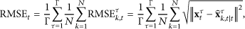$\mathrm{50}$ experiments. To evaluate the performance of the proposed d-BPF, the root-mean-square error (RMSE) is used, which is defined as

$$\begin{array}{cc}& {\mathrm{R}\mathrm{M}\mathrm{S}\mathrm{E}}_t=\frac{\mathrm{1}}{\Gamma }{\displaystyle \sum }_{\tau =\mathrm{1}}^{\Gamma }\frac{\mathrm{1}}{N}{\displaystyle \sum }_{k=\mathrm{1}}^N{\mathrm{R}\mathrm{M}\mathrm{S}\mathrm{E}}_{k,t}^{\tau }=\frac{\mathrm{1}}{\Gamma }{\displaystyle \sum }_{\tau =\mathrm{1}}^{\Gamma }\frac{\mathrm{1}}{N}{\displaystyle \sum }_{k=\mathrm{1}}^N\sqrt{{‖{\mathbf{x}}_t^{\tau }-{\widehat{\mathbf{x}}}_{k,t\hspace{0.17em}|\hspace{0.17em}t}^{\tau }‖}^{\mathrm{2}}},\end{array}$$

(49)

where Γ denotes the total number of the experiments and the term ${\widehat{\mathbf{x}}}_{k,t\hspace{0.17em}|\hspace{0.17em}t}^{\tau }$ represents the estimation of node k at time t in the τth experiment.

Figure 2

The sensor network with 50 nodes.

In this example, we use $\mathrm{32}$ box particles for the d-BPF algorithm. Figure 3 shows tracking trajectory of the d-BPF of node $\mathrm{1}$ for a single run based on measurements generated from (47). Circle marks represent the true target trajectory, while the “plus” represents the estimated trajectory. From Figure 3, it is observed that the d-BPF is able to track the trajectory of target accurately. Note that the results for different sensors are similar, and thus they are omitted here.

Figure 3

Tracking trajectory using the d-BPF with $\mathrm{32}$ box particles.

Figure 4 shows the averaged performance of the entire network over $\mathrm{50}$ Monte Carlo simulations. For performance comparison, the results of the Nc-BPF, the c-BPF, and distributed PF (d-PF) with $\mathrm{300}$ particles and $\mathrm{5000}$ particles are also presented. For clarity, the results are presented by taking the Napierian logarithm. It is observed that the d-BPF has significantly reduced the RMSE comparing to the Nc-BPF. Although it is a little inferior to the c-BPF from the viewpoint of RMSE, less communication cost is taken since the number of links is greatly smaller than that in the c-BPF.

Figure 4

Simulation results for Example 1. (a) Average position RMSE over the entire network as a function of time. (b) Average velocity RMSE over the entire network as a function of time.

The performance of the d-PF is largely dependent on the number of the particles. As shown in Figure 4, the d-BPF with only 32 box particles outperforms the d-PF with 300 particles. Although the accuracy of d-BPF is worse than the d-PF with 5000 particles, it takes much less computation time than the d-PF by using fewer box particles. It is also worth mentioning that, in order to make a comparison between d-BPF and d-PF algorithms, the noise we used in the simulation is Gaussian. It is a special case that we can use cumulative distribution function (cdf) to calculate weights so that the d-PF can deal with the interval measurements. This does not contradict with the aforementioned statement that the d-PF is in general unsuitable for the interval measurements, since the prior pdf of noise may be non-Gaussian or even unknown. However, the d-BPF can handle these cases very well. Therefore, it is where the d-BPF is expert.

4.1.2. Case 2: Dynamic Network Topology

In the second case, we simulate the d-BPF over a dynamic sensor network. In the simulation, the propagation model is also the constant velocity model defined in (45). The measurement model defined in (47) is used. We also use $\mathrm{32}$ box particles for d-BPF algorithm. Assume that all the link probabilities between two nodes are equivalent and denoted as $p_{kl}=p$ , and p keeps invariant in each simulation. Note that when p is close to $\mathrm{0}$ , the network almost reduces to a noncooperation one, that is, Nc-BPF. When $p=\mathrm{1}$ , the network is fully connected, and the result corresponds to the c-BPF.

Figures 5(a) and 5(b) show the average position RMSE and average velocity RMSE, respectively, using different link probabilities p over $\mathrm{50}$ Monte Carlo simulations, while Table 3 shows the corresponding average RMSE for $t\in [\mathrm{20,50}]$  s. From Figure 5, we can see that the performance of d-BPF over dynamic network depends on the network topology in each time slot, which is dependent on the value of the link probability p. With the increasing of p, the performance of the d-BPF is increased. Moreover, initially, when p is relatively small, for example, $p<\mathrm{0.2}$ , the average RMSE is reduced greatly compared to the Nc-BPF. After that, with the increasing of p, the performance of d-BPF improves slightly. When p is larger than about 0.6, further increasing the value of p, the performance of d-BPF does not improve much and converges to the c-BPF. It is noted that although the networks with larger link probabilities p show better estimation performance, their communication cost is also increased. Therefore, in practice, we should make a tradeoff between the estimation performance and the cost.

Table 3

Average position RMSE and velocity RMSE with different link probability p.

	Nc-BPF, $p=\mathrm{0}$	d-BPF, $p=\mathrm{0.02}$	d-BPF, $p=\mathrm{0.05}$	d-BPF, $p=\mathrm{0.1}$	d-BPF, $p=\mathrm{0.2}$	d-BPF, $p=\mathrm{0.6}$	c-BPF, $p=\mathrm{1}$
Position RMSE [m]	0.744	0.104	0.075	0.051	0.037	0.031	0.025
Velocity RMSE [m/s]	0.516	0.078	0.060	0.047	0.039	0.030	0.024

Figure 5

Simulation results for Case 2. (a) Average position RMSE over the entire network with different link probabilities p as a function of time. (b) Average velocity RMSE over the entire network with different link probabilities p as a function of time.

4.2. Example 2

In the second example, we consider the target tracking of a variable velocity model, expressed as

$$\begin{array}{cc}& {\mathbf{x}}_{t+\mathrm{1}}=\mathbf{F}{\mathbf{x}}_t+\mathbf{G}\mathbf{u}+{\mathbf{v}}_{t+\mathrm{1}}.\end{array}$$

(50)

So the target is moving with a transition density function $p({\mathbf{x}}_{t+\mathrm{1}}\hspace{0.17em}|\hspace{0.17em}{\mathbf{x}}_t)=\mathcal{N}({\mathbf{x}}_{t+\mathrm{1}},\mathbf{F}{\mathbf{x}}_t+\mathbf{G}\mathbf{u},\mathbf{Q})$ :

$$\begin{array}{cc}& \mathbf{G}={\left(\begin{array}{cccc}\mathrm{5}& \mathrm{1}& \mathrm{0}& \mathrm{0}\\ \mathrm{0}& \mathrm{0}& \mathrm{3}& \mathrm{2}\end{array}\right)}^T,\\ \mathbf{u}={\left(\begin{array}{cc}-\mathrm{0.1}& \mathrm{0.1}\end{array}\right)}^T,\end{array}$$

(51)

where F and Q are defined in (46). The measurement function g is selected the same as (47).

In the simulation, the same network as given in Figure 2 is used. The initialization and other parameters are set the same as those in Example 1. We also use $\mathrm{32}$ box particles for the d-BPF algorithm in this example.

Figure 6 shows the tracking trajectory of the d-BPF of node $\mathrm{1}$ for a single run. From Figure 6, it is observed that the d-BPF is also successful in tracking the trajectory of the target even if the velocity of target is time-varying. Figure 7 shows the averaged performance of the entire network over $\mathrm{50}$ Monte Carlo simulations. The results of the Nc-BPF, the c-BPF, and distributed PF (d-PF) are also presented. Note that the results are also presented by taking the Napierian logarithm. Similar to Example 1, it is observed that the d-BPF still significantly reduces the RMSE comparing with the Nc-BPF in this case.

Figure 6

Tracking trajectory using the d-BPF with $\mathrm{32}$ box particles.

Figure 7

Simulation results for Example 2. (a) Average position RMSE over the entire network as a function of time. (b) Average velocity RMSE over the entire network as a function of time.

5. Conclusion

In this paper, based on the traditional box particle filtering and distributed processing, we have proposed a distributed box particle filter for target tracking, namely, d-BPF, to handle the cases where the measurements are intervals-based vectors. The feasibility of the proposed d-BPF algorithm is justified. The simulations for tracking both constant and variable velocity models are carried out. From the simulation results, we find that the tracking performance of our proposed d-BPF is significantly superior to that of the Nc-BPF. Moreover, from the simulation results with a dynamic network topology, we find that the tracking performance is improved with the increasing of the link probability. It is close to the c-BPF when the link probability is much larger, while the communication cost is increased simultaneously. Therefore, in practice, we should make a balance between the tracking performance and its cost.