UAV Recharging Opportunities and Policies for Sensor Networks

Abstract

Recharging sensor networks using Unmanned Aerial Vehicles (UAVs) provides a possible method for increasing network lifetime. In this paper, we evaluate that approach, determining how much of a benefit it provides and under what conditions. We base our simulations and field experiments on data collected from charging with our UAV-based wireless power transfer system, which has similar transfer ranges and efficiencies as other such systems. We determine that a UAV can increase the network lifetime up to 290% compared to no recharging, that the UAV should recharge 30% of the sensor node battery capacity at one time for the maximum benefit, and that the UAV should recharge the lowest powered node until the network reaches a size of approximately 306 nodes at which point it should recharge the sink. We also examine how the sensor network can aid this through sink selection. The policy varies as network size increases, with a static approach working well until 200 nodes, and then either a perimeter or heuristic approach works best. These results inform future use of UAVs in recharging and working with sensor networks.

1. Introduction

Sensor networks deployed outdoors often rely on batteries for power. Long-term deployments typically require large batteries, solar cells for recharging, or periodic maintenance to replace batteries. If the network is placed in a location where traditional recharging is not effective, such as under a bridge or in a field where crop growth will obscure sun and wind, relying only on the battery capacity will limit the network lifetime significantly. To help with such scenarios, we have developed a method that allows an Unmanned Aerial Vehicle (UAV) to find [1] and wirelessly recharge sensor nodes [2], limited only by where the UAV can fly.

With our method, we want to determine how much UAV-based wireless charging actually increases the network lifetime. Does the increase in lifetime validate the addition of the recharging circuitry to the sensor nodes? If the increase is reasonable, we then want to explore under what conditions this succeeds. We focus on how much and which node the UAV should recharge. We also examine which node should act as the sink for the network data and how changing the sink can help maximize network lifetime given recharging.

To the best of our knowledge, research has not explored the benefit of UAV recharging from the sensor network perspective nor how to best utilize UAV recharging. However, significant research in the sensor network community has explored more energy efficient and cost effective hardware communication modules [3], improvement in software communication protocols [4, 5], and different data routing strategies [6–9]. An important subset has explored sink mobilization strategies [10–15].

We utilize this prior research to develop methods for the sensor network to maximize any lifetime benefits it will receive from the UAV recharging. We specifically focus on sink mobility and selected five different algorithms [16–20] from four different categories of sink mobility (static, random, controlled, and dynamic). These algorithms provide a reasonable cross section of the literature to analyze how these methods can increase network lifetime when combined with UAV recharging. Section 2.1.3 further describes these related works as we will use them within our system.

In our prior work, we modified an Ascending Technologies Hummingbird UAV to wirelessly recharge sensor nodes in a network [1, 2]. Through inductive charging, the UAV can fly out to a remote area and recharge nodes, giving a small infusion of power into the network. The UAV is able to transfer over 5 W in flight and other prototypes can transfer up to 15 W and is shown with a receiving sensor node in Figure 1. The UAV can recharge our sensor network platform, which is a custom platform consisting of a LPC2368 processor, XBee Series 1 Pro radio, and single-cell Lithium Polymer (LiPo) battery charging as shown in the bottom left of Figure 1. We charge the LiPo battery at up to 2A, depending on power available, using a LTC4001 single-cell LiPo charger.

Figure 1

UAV recharging a single node.

For this paper, we do not use the actual UAV-based wireless power transfer system as the power transfer performance has high variance that is dependent on the alignment of the coils and other factors. To ensure a fair comparison between the algorithms, we instead use the average experimentally determined power transfer rates as input to our algorithms through simulated recharging.

We begin with simulations to explore these questions in a platform-agnostic approach, introduced with preliminary explorations in [21]. The simulations allow us to determine that UAV recharging can increase the network lifetime by nearly a factor of three. We then address the other questions, determining a set of policies based on network size. These policies define which node to recharge (the sink or the lowest powered node), how much the UAV needs to recharge that node, and which node to choose as sink next. Interestingly, as network size grows, it becomes more effective to keep the sink static with the UAV recharging it by 30% at each interval. Once the network reaches 200 nodes, however, the sink should move using a heuristic-based approach.

With these results, we determine the extensions needed to implement the policies on our sensor network platform and verify the results with manual (non-UAV) recharging. The implementation consists of nine nodes and confirms the simulation results for the sink mobility algorithms plus recharging. At nine nodes, the best policy is to recharge the lowest powered node and to use a static sink approach for choosing the next sink. This work will enable better coordination between sensor networks and UAVs where the UAV can both extend the network lifetime through recharging and reduce long-range communication through data muling.

2. Materials and Methods

In this section, we describe the simulation environment used to analyze and validate our different approaches. Having introduced the environment, we discuss our different algorithms and how we use our simulations to test our algorithms. Finally, we describe our implementation on our sensor network platform as well as our experiment setup on that platform.

2.1. Simulation Environment

To explore the policies and evaluate how much recharging will help the system, we develop a simulation environment. This section outlines the assumptions in creating the simulation, the simulation structure, and the simulation operation.

2.1.1. Network Assumptions

In our model, we assume that all sensor nodes are homogeneous, with each having the capability of being the sink. We constrain our network topology to square or rectangular grids with nodes equally distributed and geographically localized with no network holes. Additionally, we assume that every node will collect the same amount of information; thus any drain in the network's energy due to sensing is the same for every node. Since our work examines the relative change in battery levels, we only focus on those operations that affect the nodes unequally, such as communication, and ignore those that affect nodes equally, such as sensing.

To generalize our results, we abstract the power and time measurements in our simulation away from hardware specifics. The battery and time measurements are not defined by real-world units, such as watt hours or seconds, respectively, but instead as an abstract definition of units. Since we are comparing relative changes for our different scenarios instead of absolute changes, this abstraction supports the comparison and ensures it holds for a range of systems.

In designing the routing system, we aim for a simple and effective scheme. Previous papers found that a multihop routing schema is the most energy efficient in transmitting data across large distances [22]. Our simulation uses Euclidean shortest distance to determine the direct neighbor that was closest to the sink. All nodes must be able to communicate bidirectionally with any of its neighbors and there is no packet loss in sending messages. No packet loss is not generally valid with wireless transmissions; however, our experiments focus on the issues of sink mobility and limited recharging where packet loss is a constant factor of the existing sent messages.

2.1.2. The Simulation

To test the objectives and theories proposed in this body of work, we created a wireless sensor network simulation in MATLAB [23]. We explored using existing sensor network simulations; however, they were either too specific to individual network platforms or more complex than needed to address our objectives.

The simulation high level block diagram can be seen in Figure 2. The first two blocks, sinkSimIter and sinkSimFunc, are the top level structures that configure the simulation parameters such as the grid topology sizes, battery unit levels, and the UAV recharge amounts.

Figure 2

Simulation flow chart.

The block sinkSim configures the physical topology of the grid and the communication connectivity between the nodes. This configuration occurs via three preprocessing modules: getBatteryCapacity, createNodeTopology, and generateConnectivity. Once the network is set up, sinkSim iterates through time units (generically defined to suit whatever the platform uses) and, at each time unit, computes four different functions: (1) sink selection for the next iteration, (2) the new routing for the new sink, (3) each node's new power level based on communication drain and any recharging, and (4) the logging of variables of interest such as battery levels. In analyzing the logged results, we define the network lifetime to be the time at which the first node in the network is completely drained of battery.

2.1.3. Sink Selection Algorithms

Periodically changing the sensor node which is the sink (the node that collects all the data from the network) is an effective way to balance energy usage in a sensor network since the sink and nodes surrounding it use more energy as they relay messages from other nodes. Research into energy conservation by specific positioning of the sink can be classified in four ways: static sink positioning, random sink movement, controlled sink movement, and dynamic sink movement. Our research looked into these four different classification categories to find the best way to select the sink in order to optimize the impact the UAV has on the network. This section discusses existing algorithms from each category and how we adapt each to our system.

(i) Static Sink Positioning. The static sink algorithm fixes the sink at a stationary location throughout the lifetime of the sensor network. Early sensor networks used this method of sink positioning and significant research explored determining the optimal position in the network [19]. The research conducted by Luo and Hubaux mathematically found that the optimal placement of a static sink was in the center of the network [18]. Our implementation of the static sink places the sink in the center.

(ii) Random Sink Movement. The work of Chatzigiannakis proved that a mobile sink moving randomly around the network increases the network lifetime compared to the static sink approach [17]. For this sink classification, we use a random function to choose the placement of the sink. The sink stays at a node for one time interval and then it uses the random function to choose the next node to become the sink.

(iii) Controlled Sink Movement. The third sink classification that this paper explores is controlled sink movement. As opposed to random sink positioning, this movement is consciously controlled and planned before the network begins operating. We examined two different approaches: a method called Circles and a Linear Programming approach.

Circles. In one algorithm proposed by Luo and Hubaux [18], moving the sink along the outermost perimeter of the network dramatically increased the network lifetime versus a static sink. Using multihop routing, this peripheral pattern of moving the sink balanced the energy load equally across the network, thus improving the lifetime. While this paper assumes a Poisson circular distribution of nodes [18], we confirmed that the approach holds for our grid topologies.

Linear Programming. Another controlled sink movement that we explore is a Linear Programming optimization, specifically an approach by Wang et al. [20]. Based on this work, we create our linear equation, denoting it to be the time that the sink stays at any one particular node. Equation (1) outlines the approach. In this equation, t represents the amount of time that node is the sink during the lifetime of the network.

We find the maximum solution to this equation by prolonging the sink's sojourn time at each node. In doing so, we maximize the network lifetime because the longer the sink stays at every node, the longer the network lifetime is.

Max network lifetime is as follows:

\begin{matrix} \sum_{\forall k \in N} t_{k} \end{matrix}

(1)

subject to

\begin{matrix} \sum_{\forall k \in N} c_{i}^{k} t_{k} \leq e_{0}, \end{matrix}

(2)

\begin{matrix} t_{k} \geq 0, \end{matrix}

(3)

where N is the set of all nodes in the grid. k represents the current sink. i represents a general node in the grid.

t_{k}

represents the sojourn time spent at each sink.

c_{i}^{k}

represents the cost of one node sending and receiving data in one time interval when the sink is at position k.

Equation (2) is our constraint that represents the cost of sending and receiving packets of information for each node when the sink is at position k, but not draining the battery more than its initial energy. This constraint represents our power limitation in the network and ensures that no battery can be drained below its capacity. Our last constraint (3) ensures that the result does not give us a negative value for a sink sojourn time. Once this optimization is completed, the algorithm creates a sink movement based on the results.

Wang et al. state that applying the Linear Programming optimization results could be implemented regardless of the order in which the sink follows the optimization [20]. The paper discusses two implementations: exact sink movement and periodic sink movement. In exact sink movement, each node remains sink for its full sojourn time before the sink transitions to the next node. For periodic sink movement, the node is sink for one time unit and then transitions to the next node. After the sink visits all nodes once, it returns to the starting node and repeats the cycle. As each node reaches its full sojourn time, it is removed from the rotation. We analyze both approaches and determine that when we have the ability to recharge, periodic sink movement provides the longest lifetime, which is what we use in our implementation of this algorithm.

Wang et al. did not consider limited recharging while implementing the optimization, which is necessary for implementation. With a linear optimization, we can only account for the energy drain as direct results of the sink's position and not directly optimize for the recharging of the UAV. Therefore, within the linear optimization, we instead adjust the cost of sending and receiving messages to reflect the variable recharge placement as an even distribution of power across all the nodes.

2.1.4. Dynamic Sink Movement

The previous sink algorithms utilize initial known variables to determine the sink selection process. This last sink algorithm category differs in that it uses the dynamically changing network energy levels to determine which node should be the next sink.

Basagni et al. found that multihop networks suffer from the so-called neighborhood problem [16]. Nodes surrounding the sink, called “neighbor” nodes, become inundated with all packets being sent to the sink. This inundation drains these nodes faster than the others farther away from the sink. Using this information, the paper creates a heuristic called Greedy Maximum Residual Energy (GMRE). This algorithm moves the sink to the section of nodes with the highest energy levels in an effort to drain the nodes energy more evenly around the network. At each iteration the algorithm calculates the highest energy grouping in the network and moves the sink to that location, knowing that the nodes around it will become more drained than the others. We utilize the same approach although we include the recharging of the node in our energy calculations.

2.2. Simulation Test Setup

In this section, we describe our experiment setup in order to determine the answers to the following questions: (i)

How much does using a UAV to recharge a node extend the network lifetime of a sensor network?

(ii)

Which node should the UAV recharge at every time unit?

(iii)

Which sink selection algorithm in combination with node recharging extends network lifetime?

We run our simulations on seven grid topologies: 8 by 8, 8 by 13, 8 by 18, 11 by 18, 14 by 18, 17 by 18, and 20 by 18. These grids were chosen because the total number of nodes in these grid sizes were near 50, 100, 150, 200, 250, 300, and 350, respectively.

2.2.1. Experiment 1: Recharging Effectiveness

We first explore the effectiveness of recharging in extending network lifetime. We run two tests over the set of topologies: one with no recharging and one with recharging. For recharging, every time unit during the simulation, the UAV recharges the sink node by 25% of the initial energy of the node.

2.2.2. Experiment 2: UAV Recharge Amount

Since the choice of 25% is somewhat arbitrary, we explore how much the UAV needs to recharge to become a viable option. The amount the UAV can recharge a node within a time unit is directly proportional to how much battery capacity the UAV needs (as well as the ability to carry that capacity). If we determine the percentage of charging needed, we can better design the UAV and sensor network platform. We use the same seven grid topologies. Over those topologies, we vary the recharge amount the sink receives from 0% to 55% of the node's initial energy.

2.2.3. Experiment 3: Node Recharging Selection

The next key objective is to find out how the UAV should recharge the network. We assume that the sink is the best node to recharge due to its large amount of communication and since, if the sink dies, the entire network becomes inoperable. However, the sink may not be the node closest to dying. Instead, we define the “lowest powered node” as the node that has the least amount of energy left in its battery at any given time unit. We set up our next experiment to see if recharging the lowest powered node improves the network lifetime compared to recharging the sink node. This experiment involves using the same seven grid topologies where one simulation recharges the sink every time unit and the other recharges the lowest powered node. We use the best recharge percentage as determined in Experiment 2.

2.2.4. Experiment 4: Sink Selection

The next key objective is to determine which sink algorithm best optimizes the limited recharging capability of the UAV. For our experiments, we implement our sink algorithms discussed in Section 2.1.3, adjusting for our network constraints and grid topologies. We then compare the results to determine which algorithm works best in conjunction with the UAV recharging. For our test setup, we run the simulations on the same seven grid topologies, use our results from Experiment 2 to determine the best recharge amount, and use our results from Experiment 3 for selecting the sink versus the lowest powered node.

2.3. Sensor Network Environment

In this work, we use the SEAM sensor network platform that we developed in prior work [24]. The SEAM platform is modular, allowing easy additions of the custom wireless power receiving systems. The SEAMos software [25] already supports the core hardware and has libraries for the UART, logging, SD card, and an event scheduler. The experiment uses three libraries (xbee, sink, and node power) in order to control different aspects of the sink selection and sensor node hardware.

The xbee library controls the transmission and reception of information over the XBee radio. It develops a packet structure for the messages that are sent between the nodes. Each message contains the transmitting node ID, the destination node ID, the type of message being sent, the node from which the message originated, the power level of the origin node, the current sink iteration, and a message terminator. When a node receives a message, a function from this library interprets the message and performs one of four actions: (1) schedule a new sink selection process if that node is the next sink, (2) schedule a send-to-sink process if the system has selected a new sink that is not the current node, (3) forward the message, or (4) ignore the message. The system logs all received and transmitted messages as part of the experiment.

The xbee library also deals with the issues of synchronizing and back-off procedures. Synchronizing occurs upon start with the sink sending a time interval message to all other nodes. For the back-off procedures, each node schedules its processes after the “new sink” message is sent or received by a node. All messages to send in a process are delayed by 0.02 intervals multiplied by its ID to ensure distinct transmission windows.

The sink library consists of the actual experiment functions. It stores the node ID number, ID of the sink, number of rows and columns in the network grid, and the sink and recharge algorithms to use. When it is time for a node to send its message to the sink, a function determines to which node it must send its message in order to reach the sink. If the current node is the sink and it is time to select a new sink, the sink selection function runs the current sink selection algorithm as well as the recharge algorithm. Sink selection requires changes compared to the simulation. The simulation assumes all nodes know the new sink without additional communication. However, the platform requires actual communication of this information. To achieve this, the sink uses the multihop routing protocol to transmit a “new sink” message to the nodes. With this additional message, the sink's power level decrements by one additional power unit and all other nodes’ levels decrement by two additional power units compared to the simulation.

Finally, the node power library tracks the pseudo power level of each node during the experiment. All nodes start at a maximum level and, as they send and receive messages, the power level decreases. If the node will be recharged in a given time interval, it adds a set amount of energy to its power level with a ceiling of the maximum starting level. Along with tracking its own power, each node tracks the power of the other nodes. This allows the node, when it becomes the sink, to choose the next sink during the Greedy sink algorithm experiment. It also allows the nodes to determine, in a decentralized manner, who is the lowest powered during the lowest powered node recharging.

2.4. Sensor Network Test Setup

The experiments use nine nodes arranged in a 3 by 3 grid. Each node is about one foot away from its neighbors. Figure 3 shows a condensed example of the sensor network, with each node labeled and in the same position as during the experiments. As with the simulations, each node knows its neighbors in advance.

Figure 3

Experimental setup of sensor network.

To ensure a fair comparison (without the variances in true charging rates), we do not use the UAV to recharge; each node “recharges” by updating its known power level by the recharge value. The simulation identifies a recharge value of 30% of the starting node power level as the best level. However, with the node density used in the experiment, this is far too high to ensure that the network dies within a reasonable time frame. Instead, we use a recharge value of 0.5% of the initial power level, which are 100 and 2000, respectively. Messages require 1 power unit to send, allowing the values to remain integers in the implementation.

At the start of each experiment, each node loads configuration data from an SD card that stores the node ID, the ID of the initial sink node, the size and configuration of the network, the sink and recharging algorithms to use, and the predetermined sink path when using the Linear Programming sink algorithm. The nodes then wait in standby until they receive the message from the sink to start each experiment. As each experiment runs, each node logs every message it transmits or receives, even if the message received is for a different node. When the node's pseudo power level reaches zero, that node transmits a message to all other nodes and the experiment stops.

We perform two experiments on the platform, duplicating the experiments in the simulations to help translate those results into platform-based scenarios. The first experiment validates the results from Experiments 1 and 3 in the simulation. The sensor network first runs with no recharging and the static sink selection algorithm. Upon the death of the first node, the test stops and we collect the data from the sensor nodes. We repeat this process with recharging the sink and static sink as well as recharging the lowest powered node and static sink. We select a recharge amount of 0.5% of the initial power level for this experiment.

The second experiment tests the five sink selection algorithms. The objective of this experiment is to verify the results of Experiment 4 in the simulations. Each test uses the same network grid topology and uses the lowest powered node recharge algorithm with a 0.5% recharge amount at each sink interval. For each sink algorithm, the network runs until the death of the first node. After that, we collect the data and restart the network.

3. Results and Discussion

In this section, we outline the results from our simulation and sensor network experiments that we described in Sections 2.2 and 2.4. For each experiment, we analyze and discuss the results immediately after presenting them.

3.1. Simulation Results

Given our network setup and constraints, we ran the simulation to gather data to help us determine the answers to our three key objectives: (1) how much benefit to receive from recharging with the UAV, (2) which node to recharge, and (3) which sink selection algorithm to use.

3.1.1. Experiment 1: Recharging Effectiveness

Our first experiment explores the effectiveness of recharging in extending network lifetime. Table 1 reflects the impact of recharging versus no recharging. The results are displayed as the overall network lifetime, which is the time unit when the first node failed.

Table 1

Recharging performance for different node configurations.

Grid topologies	Total number of nodes	Network lifetime
Grid topologies	Total number of nodes	No recharging	Recharging
8 by 8	64	17	66
8 by 13	104	11	33
8 by 18	144	8	20
11 by 18	198	7	16
14 by 18	252	5	15
17 by 18	306	5	14
20 by 18	360	4	8

These results show that the there is a positive impact on network lifetime. This impact ranges from a 100% increase in lifetime to a 290% increase.

The results also indicate that as the number of nodes increases, the impact that the UAV has on the network lifetime decreases. When the number of nodes increases, the amount of communication and, therefore, energy used increases; however, the UAV's recharge amount does not change. This results in a decrease in the ratio of recharge to energy drain of the network; thus recharging impacts the network less as the network gets larger.

3.1.2. Experiment 2: UAV Recharge Amount

Our second experiment explores the amount that the UAV recharges. The results can be seen in Figure 4.

Figure 4

Multiple grid topologies with varying recharge amounts: recharging the sink.

When the UAV recharges below 30 percent of a node's initial energy, the network lifetime suffers. At and above 30 percent, the network lifetime does not change and stays constant. Since there is no positive impact on the network lifetime if the UAV charges more than 30 percent, but a negative cost to the UAV in terms of battery carrying capacity, there is no need for the UAV to recharge more than 30%, making it the best recharge amount.

In Table 2, you can see the network lifetime as the time until the first node failed. Again, it is important to note that as the network grows, the impact of the UAV decreases because the ratio of energy the UAV can provide decreases. Most topologies see the same results.

Table 2

Static sink with 30% recharging.

Grid topologies	Total number of nodes	Network lifetime
8 by 8	64	66
8 by 13	104	33
8 by 18	144	20
11 by 18	198	16
14 by 18	252	15
17 by 18	306	14
20 by 18	360	12

3.1.3. Experiment 3: Node Recharging Selection

The next key objective is to determine how the UAV should recharge the network. Based on our results from Experiment 2, we use a recharge percentage of 30%. The results of this test are shown in Table 3. The simulation ran for a total of 200 time units; any result that has a network lifetime of 200 never saw a node die.

Table 3

Recharging the sink versus recharging the lowest powered node.

Grid topologies	Total number of nodes	Sink recharged	Lowest powered node recharged
8 by 8	64	66	200
8 by 13	104	33	200
8 by 18	144	20	42
11 by 18	198	16	28
14 by 18	252	15	19
17 by 18	306	14	17
18 by 18	324	14	13
19 by 18	342	14	11
20 by 18	360	12	10
22 by 18	396	9	9
20 by 20	400	9	9

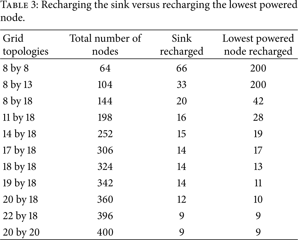
At grid sizes between 306 nodes and 324 nodes, the most effective recharging schema switches from the lowest powered node to the sink. We graphed the impact of recharging the sink versus recharging the lowest powered node versus the number of nodes in the network, as seen in Figure 5. The results show that the impact of recharging the network drops off exponentially as a function of the number of nodes in the network. These results also show that the lowest powered node drops off faster than recharging the sink and, around 306 nodes, recharging the sink becomes better than recharging the lowest powered node.

Figure 5

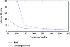
Decreasing impact of recharging as the number of nodes in the network increase.

This result was not unexpected. As the number of nodes increases, the amount of packets the sink has to forward to the UAV increases to a value exponentially larger than the number of packets the neighboring nodes send. This results in the sink becoming the node that requires the most energy. At these times in the network, the sink is not the lowest powered node. However, one time unit later, passing along those packets without any recharging of the sink will cause the sink to lose power completely and the network to die. Recharging the sink in this situation, then, extends the network lifetime more than recharging the lowest powered node. For the rest of our experiments, any topology with 307 or more nodes will recharge the sink and any topology smaller will recharge the lowest powered node.

3.1.4. Experiment 2 (Again): Revisiting Recharge Amount

Experiment 2 explored the amount that the UAV should recharge when recharging the sink. Now that we have modified our recharging policy, we revisit the question posed in Experiment 2 and determine the percentage that the UAV should recharge as a ratio of the initial node's energy. Figure 6 shows that the UAV's recharge amount depends on the number of nodes in the network. As the network size increases, the amount the UAV should recharge increases.

Figure 6

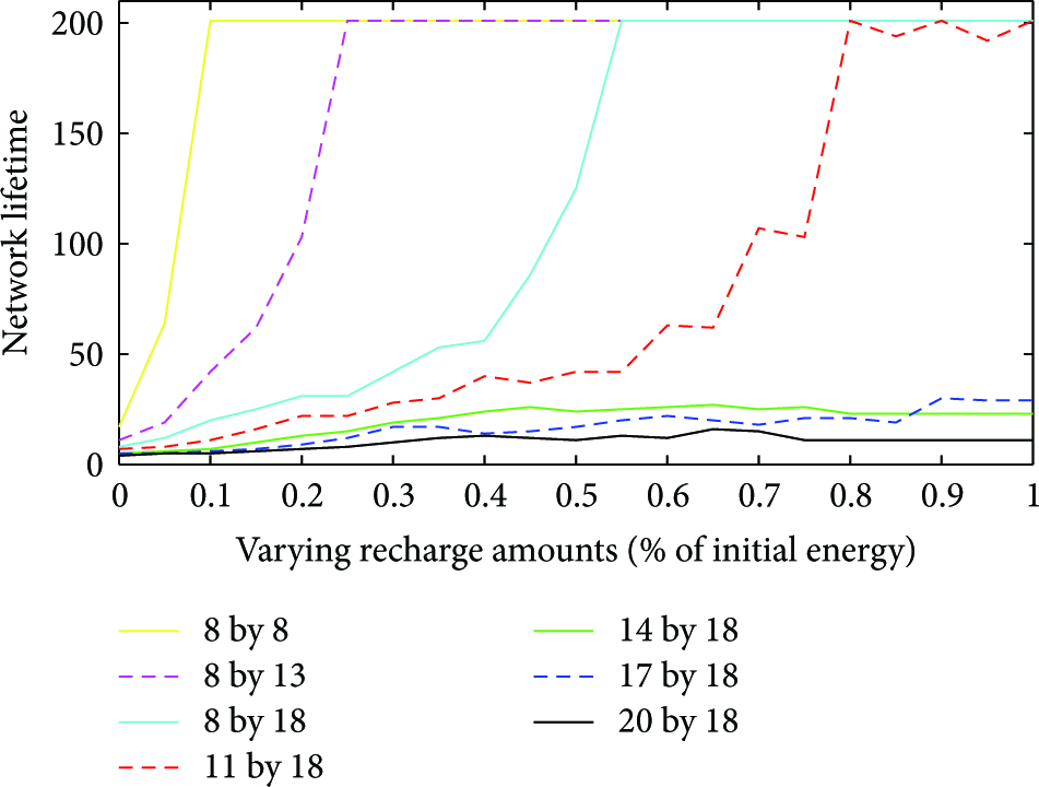
Multiple grid topologies with varying recharge amounts: recharging lowest powered node.

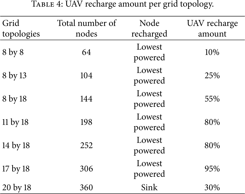
Table 4 describes the recharge amount at which the UAV has the largest impact for each grid topology along with the policy defined in Experiment 3. These results are shown as a percentage of the initial node's energy. Based on the results in the table, for those networks following a lowest powered policy, the UAV recharge amount is a function of the number of nodes in the network. However, when changing to a sink policy, as shown in the 20 by 18 grid size, we revert back to the 30% seen in the first Experiment 2. Recharging the sink for larger grid sizes, therefore, not only reduces computational complexity compared to determining the lowest powered node, but also reduces the amount of battery capacity that the UAV must carry.

Table 4

UAV recharge amount per grid topology.

Grid topologies	Total number of nodes	Node recharged	UAV recharge amount
8 by 8	64	Lowest powered	10%
8 by 13	104	Lowest powered	25%
8 by 18	144	Lowest powered	55%
11 by 18	198	Lowest powered	80%
14 by 18	252	Lowest powered	80%
17 by 18	306	Lowest powered	95%
20 by 18	360	Sink	30%

3.1.5. Experiment 4: Sink Selection

The next key objective is to determine which sink algorithm best optimizes the limited recharging capability of the UAV. For our experiments, we implement our sink algorithms discussed in Section 2.1.3, adjusting for our network constraints and grid topologies. We then compare the results to determine which algorithm works best in conjunction with the UAV recharging. For our test setup, we ran the simulations on the same seven grid topologies from before and use our results from Table 4 for policy selection.

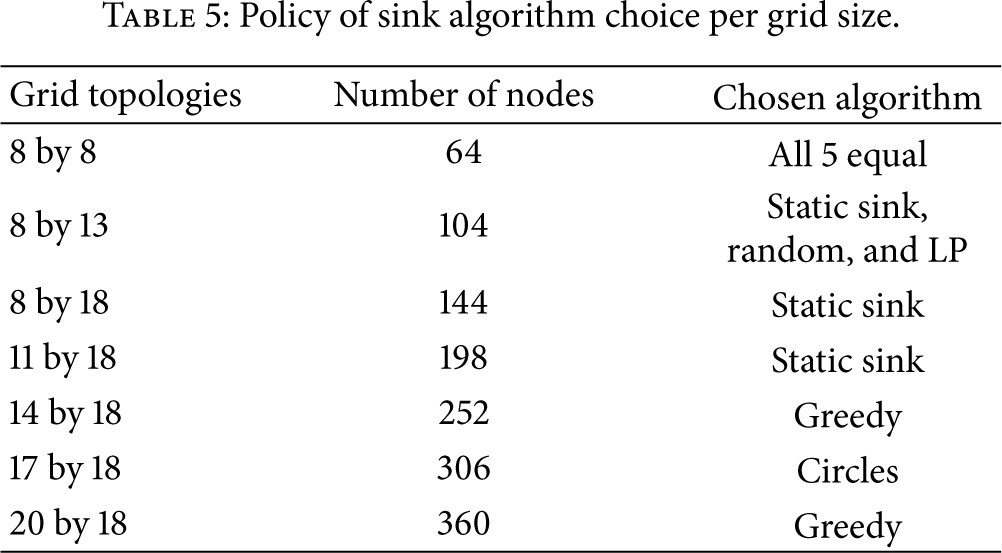
Figure 7 shows the results of this experiment while Table 5 describes our sink algorithm policy for a given grid size, based on these results. The first grid size, 8 by 8, never fails during the simulation due to recharging sufficiently balancing all nodes within the 200 time units.

Table 5

Policy of sink algorithm choice per grid size.

Grid topologies	Number of nodes	Chosen algorithm
8 by 8	64	All 5 equal
8 by 13	104	Static sink, random, and LP
8 by 18	144	Static sink
11 by 18	198	Static sink
14 by 18	252	Greedy
17 by 18	306	Circles
20 by 18	360	Greedy

Figure 7

All five sink positioning algorithms compared.

The 8 by 18 and 11 by 18 grid sizes have the longest network lifetimes when using the static sink. This is surprising because all papers on sink positioning algorithms say that the static sink performs poorly. However, with our added dimension of recharging, the reason the static sink outperforms all other algorithms is the same reason that it performs the worst without recharging. These grid sizes recharge the lowest powered node. They experience the neighborhood problem where the nodes around the sink die the fastest, but the UAV manages to recharge these nodes fast enough to ensure the network continues to operate. The other sink algorithms move the sink around, which increases the number of nodes needing recharging beyond the UAV's ability to support those nodes.

At grid sizes larger than 200 nodes, the UAV can no longer recharge enough energy to compensate for the energy drain in the neighbors. Thus, the best performing sink positioning algorithms for the larger three grid sizes are the Greedy and Circles algorithms. To choose an appropriate sink algorithm, we could follow Table 5 or consider other factors such as time/space complexity or ease of implementation.

3.2. Sensor Network Results

In this section, we describe the results of the two experiments described in Section 2.4. Overall we find that the sensor network implementation matches the simulation results, with the static sink performing the best, although Greedy approach performs somewhat better due to the overall number of packets sent during the simulation versus the experiment.

3.2.1. Recharging Effectiveness and Selection

Figure 8 shows the results of no recharging, sink recharging, and lowest powered node recharging. Overall the simulation shows significantly longer network life for each algorithm, which is caused by the additional messages sent by the sensor network implementation as we described in Section 2.3. The relative lifetime between these different approaches, however, is the same for simulation and implementation.

Figure 8

Comparison of three recharge algorithms in simulation and experiments.

3.2.2. Sink Selection

We next confirmed the sink selection results. Figure 9 describes these results. Most algorithms performed comparable to the simulation; however, Greedy performs better in implementation than simulation.

Figure 9

Comparison of five sink algorithms in simulation and experiments.

Figures 10 and 11 demonstrate why Greedy performs better in the experiment. As seen in Figure 10, for the simulation, Node 4 was the sink for the majority of the simulation experiment with Nodes 3 and 9 being the sink for the second and third largest amount of time, respectively. In Figure 11, for the sensor platform, Node 4 was still the sink for the majority of the experiment, but Node 5 was the sink for the second largest amount of time and no other node was sink for a significant portion of time. This is significantly more often than in the simulation, at about one-third of the experiment. Since Node 5 is situated in the center of the 3 by 3 network grid, all nodes are neighbors of Node 5 and no message forwarding needs to occur with any of the nodes. This lack of forwarding results in a decrease in the number of packets sent or received during the time that Node 5 is the sink compared to any other node as sink. Less messages signify an overall decrease in energy drain during the experiment, allowing the network to live for a longer time relative to the other sink algorithms.

Figure 10

Times as sink and times recharged during simulation of Greedy algorithm.

Figure 11

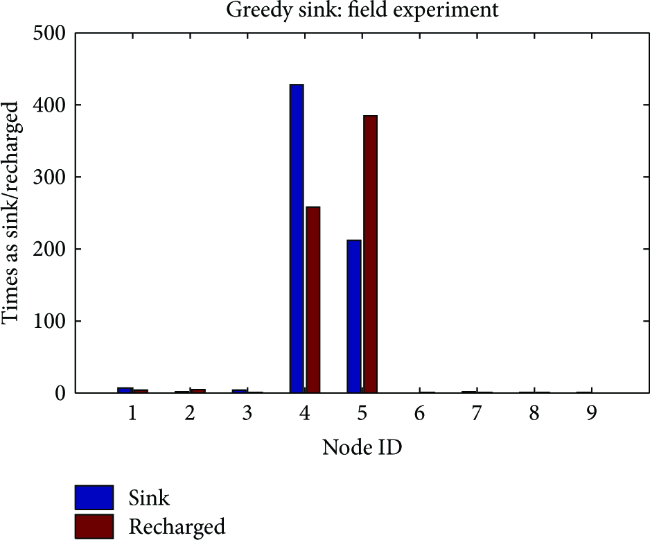
Times as sink and times recharged during experiment of Greedy algorithm.

4. Conclusion

In this work we explore the utility of using UAVs with wireless power transfer systems to recharge wireless sensor networks. We present simulations and sensor network experiments that determine that a UAV can improve the lifetime of a sensor network by as much as 290%. This works best by having the UAV recharge the system by 30% of the battery capacity of a node, having the UAV recharge the lowest powered node until the network size exceeds 306 nodes, and having the sensor network use a static sink until the network size exceeds 200 nodes where it should switch to Greedy or Circles approaches for sink selection. We verify the simulations through field experiments with nine nodes and find that, even with the slight algorithm modifications needed for field experiments, the results match. The only exception is the Greedy algorithm which performed slightly better in the field experiments due to the different number of packets sent and received by the sensor nodes.

The simulations and sensor network experiments in this work were performed with energy and charging data from our UAV-based wireless power transfer system developed in our prior work. The algorithms and findings, however, are generalizable to other UAV systems that charge sensor networks and inform the future deployments of UAV and sensor network systems.

Moving forward, we plan to evaluate the algorithms in more extensive field deployments, investigate the development of mathematical bounds on the sink selection, and also aim to incorporate data muling into the policies. Adding the UAV recharging into the system will require expanding our communication protocol between the UAV and sensor network to tell the UAV which node to recharge; upon installation of the nodes, we will record the GPS coordinates of each node, which will allow the UAV to find a specific node.

Footnotes

Conflict of Interests

The authors have no conflict of interests that impact the validity of this research or its results.

Acknowledgments

The authors are grateful for NSF CNS (CSR-1217400 and CSR-1217428) and NSF RI (IIS-1116221), which partially supported this work.

References

Mittleider

Griffin

Detweiler

Experimental analaysis of a uav-based wireless power transfer localization system

Proceedings of the International Symposium on Experimental Robotics (ISER ′14)

June 2014

Marrakech, Morocco

Griffin

Detweiler

Resonant wireless power transfer to ground sensors from a UAV

Proceedings of the IEEE International Conference on Robotics and Automation (ICRA ′12)

2012

2660 2665

10.1109/icra.2012.6225205

2-s2.0-84864479907

Zhao

Guibas

L. J.

Wireless Sensor Networks: An Information Processing Approach 2004

Boston, Mass, USA

Morgan Kaufmann

Kim

Shin

Cha

Y-MAC: an energy-efficient multi-channel MAC protocol for dense wireless sensor networks

Proceedings of the International Conference on Information Processing in Sensor Networks

April 2008

St. Louis, Mo, USA

53 63

10.1109/ipsn.2008.27

2-s2.0-51249088899

Heidemann

Estrin

An energy-efficient MAC protocol for wireless sensor networks

Proceedings of the 21st Annual Joint Conference of the IEEE Computer and Communications Societies

June 2002

1567 1576

10.1109/infcom.2002.1019408

2-s2.0-0036343658

Akkaya

Younis

Bangad

Sink repositioning for enhanced performance in wireless sensor networks

Computer Networks 2005 49 4 512 534

10.1016/j.comnet.2005.01.014

2-s2.0-24344473784

Baruah

Urgaonkar

Krishnamachari

Learning-enforced time domain routing to mobile sinks in wireless sensor fields

Proceedings of the 29th Annual IEEE International Conference on Local Computer Networks (LCN ′04)

November 2004

525 532

10.1109/lcn.2004.71

2-s2.0-20544460077

Garcia-Luna-Aceves

J. J.

Spohn

Source-tree routing in wireless networks

Proceedings of the 7th International Conference on Network Protocols (ICNP ′99)

November 1999

IEEE

273 282

10.1109/ICNP.1999.801950

2-s2.0-0033330414

Kim

H. S.

Abdelzaher

T. F.

Kwon

W. H.

Minimum-energy asynchronous dissemination to mobile sinks in wireless sensor networks

Proceedings of the 1st International Conference on Embedded Networked Sensor Systems (SenSys ′03)

November 2003

193 204

2-s2.0-18844401338

10.

Basagni

Carosi

Melachrinoudis

Petrioli

Wang

Z. M.

Protocols and model for sink mobility in wireless sensor networks

ACM SIGMOBILE Mobile Computing and Communications Review 2006 10 4 28 30

11.

Chen

MEMOSEN: multi-radio enabled mobile wireless sensor network

Proceedings of the 20th International Conference on Advanced Information Networking and Applications

April 2006

291 295

10.1109/aina.2006.213

2-s2.0-33751073973

12.

Hou

Y. T.

Shi

Sherali

H. D.

Optimal base station selection for anycast routing in wireless sensor networks

IEEE Transactions on Vehicular Technology 2006 55 3 813 821

10.1109/tvt.2006.873822

2-s2.0-33744551994

13.

Kim

Lee

Rim

3DE: selective cluster head selection scheme for energy efficiency in wireless sensor networks

Proceedings of the 2nd International Conference on PErvasive Technologies Related to Assistive Environments (PETRA' 09)

June 2009

33:1 33:7

10.1145/1579114.1579147

2-s2.0-70450231829

14.

Lee

Wicke

Kusy

Gnawali

Guibas

Data stashing: energy-efficient information delivery to mobile sinks through trajectory prediction

Proceedings of the 9th ACM/IEEE International Conference on Information Processing in Sensor Networks (IPSN '10)

April 2010

Stockholm, Sweden

291 302

10.1145/1791212.1791247

2-s2.0-77954500917

15.

Marta

Cardei

Improved sensor network lifetime with multiple mobile sinks

Pervasive and Mobile Computing 2009 5 5 542 555

10.1016/j.pmcj.2009.01.001

2-s2.0-70349771047

16.

Basagni

Carosi

Melachrinoudis

Petrioli

Wang

Z. M.

Controlled sink mobility for prolonging wireless sensor networks lifetime

Wireless Networks 2008 14 6 831 858

10.1007/s11276-007-0017-x

2-s2.0-54149084958

17.

Chatzigiannakis

Kinalis

Nikoletseas

Efficient data propagation strategies in wireless sensor networks using a single mobile sink

Computer Communications 2008 31 5 896 914

10.1016/j.comcom.2007.12.011

2-s2.0-40249089977

18.

Luo

Hubaux

J.-P.

Joint mobility and routing for lifetime elongation in wireless sensor networks

Proceedings of the IEEE 24th Annual Joint Conference of the IEEE Computer and Communications Societies

March 2005

1735 1746

2-s2.0-25844459686

19.

Safwat

Hassanein

Mouftah

Power-aware virtual base stations for wireless mobile ad hoc communications

Computer Networks 2003 41 3 331 346

10.1016/s1389-1286(02)00419-x

2-s2.0-0037458438

20.

Wang

Z. M.

Basagni

Melachrinoudis

Petrioli

Exploiting sink mobility for maximizing sensor networks lifetime

Proceedings of the 38th Annual Hawaii International Conference on System Sciences (HICSS ′05)

January 2005

287

2-s2.0-27544435369

21.

Johnson

Basha

Detweiler

Charge selection algorithms for maximizing sensor network life with UAV-based limited wireless recharging

Proceedings of the 8th International Conference on Intelligent Sensors, Sensor Networks and Information Processing (ISSNIP ′13)

April 2013

159 164

10.1109/issnip.2013.6529782

2-s2.0-84881118835

22.

Yaacoub

Abu-Dayya

Matin

D. M.

Multihop routing for energy efficiency in wireless sensor networks

Wireless Sensor Networks—Technology and Protocols 2012

Berlin, Germany

Springer

165 188

23.

The MathWorks MATLAB Release 2010

Natick, Mass, USA

The MathWorks

24.

Basha

Detweiler

Doniec

Vasilescu

Rus

Using a multi-functional sensor network platform for large-scale applications to ground, air, and water tasks

Proceedings of the 6th Workshop on Hot Topics in Embedded Networked Sensors (HotEmNets '10)

June 2010

ACM

10.1145/1978642.1978662

2-s2.0-79959345189

25.

SEAMos Repository: Seam operating system, https://code.google.com/p/seamos/