NDSL: Node Density-Based Subregional Localization in Large Scale Anisotropy Wireless Sensor Networks

Abstract

Localization is emerging as a fundamental component in wireless sensor network and is widely used in the fields of environmental monitoring, national defense and military, transportation, and so on. Current positioning system, however, can only locate an object's position in isotropy wireless sensor network with high accuracy but cannot locate it accurately in anisotropy wireless sensor network. Besides, past proposals only mentioned anisotropy to show that connectivity of network is different in each direction. However, how to quantify the degree of anisotropy is not clearly pointed out. This paper introduces NDSL (node density-based subregional localization), a positioning system that is used in anisotropy wireless sensor network. The network is divided into many subregions where the nodes density is relatively uniform and then corrects the single-hop distance for each beacon node to locate unknown nodes. We also use nodes distribution and signals distribution to build a model to evaluate the degree of anisotropy for anisotropy network. Through the analysis of the degree of anisotropy for different topologies, the results show that the model is consistent with the facts. Results from actual deployments and simulation experiments show that the accuracy of NDSL algorithm obviously improves compared with DV-Hop algorithm.

1. Introduction

Network is always anisotropic because of random deployment of nodes, interferences of wireless signals, breakdown of nodes, conflict of communication, and so on. Nodes localization in anisotropy network is always a challenge. Current positioning systems, however, can only locate an object's position in isotropy wireless sensor network with high accuracy but cannot locate it accurately in anisotropy network. Many applications, however, would benefit from knowing the objects' accurate positions in anisotropy network. For example, for conservation of earthen ruins, the monitoring nodes are deployed differently in different areas; thus the monitoring network is an anisotropy network and the positions of damaged ruins need to be obtained as soon as possible to get immediate protection [1, 2].

Nodes localization in anisotropy network has recently received much attention [3–8]. DV-Hop algorithm [9] is widely used in large scale anisotropy network for nodes localization because of its simple implementation and low requirements for hardware. However, DV-Hop algorithm suffers from low accuracy and high dependence on topologies. Some researchers [10–13] try to augment DV-Hop algorithm in single-hop distance, hop counts, and position calculation. However, underlying those improving methods is an assumption that the nodes distribution in network is even, which is unlikely in most practical nodes' setups. Anisotropy network occurs when the nodes need to be deployed differently according to practical situations (such as in conservation of earthen ruins). That anisotropy is inevitable in practice and is exacerbated in a network that is full of strong protection areas and weak protection areas. Indeed, anisotropy is the natural mode of operation for nodes localization.

This paper introduces NDSL (node density-based subregional localization), a positioning system that works in anisotropy wireless sensor network and we also build a model to evaluate the degree of anisotropy for anisotropy wireless sensor network. In line with common practice in locating objects, NDSL employs beacon nodes, whose positions are known a priori.

Unlike past approaches, which only mentioned anisotropy to show that connectivity of network is different in each direction, however, the degree of anisotropy is not clearly pointed out [3, 14]. In this paper, we build a model to evaluate the degree of anisotropy for anisotropy network. The model is built according to nodes distribution and signals distribution. For nodes localization in anisotropy network, past proposals always used DV-Hop algorithm in the whole network. Unlike DV-Hop algorithm, for NDSL algorithm, the network is divided into many subregions, where in each subregion the nodes density is relatively uniform, as shown in Figure 1. Then the single-hop distance for each subregion will be corrected and the unknown node is located with corrected single-hop distance to get better accuracy.

Figure 1

Regional division in anisotropy network. Nodes density in each subregion is relatively uniform. The communication between beacon node in subregion A and beacon node in subregion C may go through subregion B.

To illustrate NDSL's approach, Figure 1 shows a simple example with three subregions, where in each subregion the nodes density is relatively uniform. As Figure 1 shows, the nodes density in the whole network is nonuniform, although in each subregion the nodes density is uniform; thus the whole network in Figure 1 is anisotropic. In isotropy network, mean single-hop distance can be seen as the single-hop distance of beacon nodes in the whole network. However, in anisotropy network, the single-hop distance of each beacon node is very different because of nonuniform nodes distribution and signals distribution. For example, in Figure 1, the single-hop distances in areas A, B, and C are different. When the distance between beacon node and unknown node is calculated as mean single-hop distance times hop counts, the calculated position of unknown node will not be the actual position, and it varies widely. So the single-hop distance needs to be recalculated in anisotropy network. The localization error will be decreased by recalculated single-hop distance of each beacon node for each subregion.

So how can we automatically divide a large scale anisotropy network and calculate single-hop distance of each beacon node for each subregion? To do so, we need to divide the network according to nodes distribution. In contrast to the illustrative example, however, real-world deployment has many circumstances, such as environmental disturbance, and using nodes density to divide the network is not enough. Further, because signals broadcast irregularly in different environments, sometimes the far node is the neighbor of beacon nodes. In designing a technique that divides the network in a relatively accurate way, the network is divided according to nodes density and RSSI sequence of neighbors. First, the number of neighbor nodes is corrected using RSSI sequence of neighbors and more accurate number of neighbor nodes can be obtained through the choice of nodes' RSSI. Then the comparison of the number of neighbor nodes between node i and node j is done to make sure whether they are in the same subregion. After the comparison, the network will be divided into many subregions automatically and accurately, and the nodes density in each subregion is relatively uniform. We present details of NDSL algorithm in Section 4 and in Section 5 demonstrate that the localization error of NDSL algorithm decreases obviously, compared to DV-Hop algorithm.

The contributions of this paper are as follows:

• (i)

This paper proposes a model to evaluate the degree of anisotropy for anisotropy network, and the model provides the reference for the evaluation of anisotropy network.

(ii)

The network is divided according to RSSI sequence of neighbors and the number of neighbors to improve the accuracy of regional division.

(iii)

This paper proposes NDSL algorithm, a regional division algorithm according to nodes density to locate unknown nodes with better accuracy compared to DV-Hop algorithm in large scale anisotropy network. To our knowledge, NDSL is the first work to use regional division to locate nodes in large anisotropy network.

The rest of this paper is organized as follows: Section 2 will introduce related work, and the model for evaluation will be presented in Section 3; this is followed by subregional division in Section 4. Section 5 will introduce the nodes localization algorithm NDSL, and test-based results will be showed in Section 6. Section 7 will show the simulation results; then conclusion will be introduced in Section 8.

2. Related Work

The existing researches on localization can be classified into two main categories: range-based localization and range-free localization. Range-free approaches, such as centroid [15], MDS-MAP [16], and DV-Hop [17], mainly rely on connectivity measurements, that is, from beacon nodes to unknown nodes, such as hop counts. Since the connectivity measurements are easily affected by nodes density and network conditions, range-free approaches typically provide imprecise estimation of nodes' positions.

Range-based approaches [18–24] measure the Euclidean distances among the nodes with certain ranging techniques and locate the nodes using geometric methods, such as TOA [25], TDOA [26], and AOA [27, 28]. All those approaches require extra hardware support.

Underlying above localization methods is an assumption that the network topology is isotropic: the properties of connectivity measurements are identical in all directions. In anisotropy network, the localization error is very big using the localization methods that are mentioned above. Researchers propose a series of solutions. Li and Liu [14] proposed a localization algorithm REP that is based on labeled path for hollow network, and the algorithm can estimate the Euclidean distance between pending nodes and beacon nodes more accurately in anisotropy network. However, REP algorithm is used in the network where the nodes density is very high. Wang et al. [29] proposed a localization algorithm LAEP that exploited expected hop counts and also analyzed the expected hop counts in the anisotropy network and then proposed a model to effectively increase the localization accuracy. However, the model is complicated. Unlike the methods mentioned above, Lim and Hou [30] proposed a localization algorithm that considers the nodes density and signal transmission model in actual deployment. However, the algorithm is better in the network where the nodes density is uniform.

3. Build the Model for Evaluating the Degree of Anisotropy for Anisotropy Network

3.1. Build the Model according to the Number of Neighbor Nodes

In networks, the nodes density is usually computed as the following equation:

$$\begin{array}{cc}& \rho =\frac{N}{S_{qu}},\end{array}$$

(1)

where ρ represents the nodes density, while N and $S_{qu}$ represent separately the nodes' number in the whole network and the area of the network. As shown in Figure 2, the nodes' number and the area of the four regions are all the same while the topologies of the nodes in four regions are different. According to (1), the nodes densities in four regions should be equal; however, the nodes densities are unequal in fact and the degree of uniformity of four regions is $a>d>b>c$ . As shown in Figure 2(c), the nodes density in the central area of the region is uniform while in the whole region it is nonuniform. So (1) cannot describe the nodes density of the network effectively. Nagpal [31, 32] has proposed amorphous localization algorithm, and it pointed out that when the communication range is fixed, the single-hop distance can be expressed as a function of the number of neighbors. Based on that, we propose a method that uses the number of neighbors to divide the region; that is variance grid method.

Figure 2

Different topologies with the same number of nodes. The numbers of nodes in (a), (b), (c), and (d) are all 25, the lengths of a side for four regions are all 20 m, and the areas of four regions are all 400 m², while the topology of four regional networks is different.

Before showing specific steps of variance grid method, first, a simple description of how to compute population variance and sample variance is given. Assume that there are N nodes in the network, and the neighbors' number of each node is expressed by $Y_{\mathrm{1}},Y_{\mathrm{2}},\dots ,Y_N$ . Then, the nodes distribution in the network can be expressed by variance, and the variance can be computed as follows:

$$\begin{array}{cc}& s^{\mathrm{2}}=\frac{\mathrm{1}}{N-\mathrm{1}}{\displaystyle \sum }_{n=\mathrm{1}}^N{\left(Y_i-\bar{Y}\right)}^{\mathrm{2}},\end{array}$$

(2)

where $\bar{Y}=\left(\mathrm{1}/N\right){\sum }_{i=\mathrm{1}}^N{Y}_i=Y/N$ and $Y={\sum }_{i=\mathrm{1}}^N{Y}_i$ .

The neighbors' number of M sample nodes is expressed by $y_{\mathrm{1}},y_{\mathrm{2}},\dots ,y_M$ , where $y_i$ is an element of $Y_{\mathrm{1}},Y_{\mathrm{2}},\dots ,Y_N$ . So sample variance can be computed as follows:

$$\begin{array}{cc}& s^{\prime \mathrm{2}}=\frac{\mathrm{1}}{n-\mathrm{1}}{\displaystyle \sum }_{i=\mathrm{1}}^n{\left(y_i-\bar{y}\right)}^{\mathrm{2}},\end{array}$$

(3)

where y and $\bar{y}$ represent separately the total number of samples' neighbor and the average number of samples' neighbor. The sample variance can be used to estimate population variance, and the estimation of population variance is computed as $\widehat{s^{\prime \mathrm{2}}}=s^{\mathrm{2}}$ .

Then a detailed description of variance gird method is given and the specific steps are as follows.

(i) Random Sampling. The random samples are chosen by draw method, and the N nodes can be seen as labels with number 1~N. M random numbers will be chosen from those labels and the group of the chosen labels' nodes can make up the group of samples. So the distribution of samples can be used to estimate the distribution of nodes in the whole network and also can be used to estimate the degree of nonuniformity of the whole network. The estimation lays a foundation for the next step regional division. Considering computational overhead and accuracy of estimation, the value of M is set $M=\mathrm{10}\%N$ .

(ii) Regional Division for the First Time. The whole network can be divided into t regions at first step by computing the neighbors' number of M nodes, and an example of division is shown in Figure 3; that is,    $S=\{S_{\mathrm{1}},S_{\mathrm{2}},\dots ,S_t\},\hspace{0.17em}\hspace{0.17em}{S}_i\bigcap S_j=\varnothing ,\hspace{0.17em}\hspace{0.17em}i\ne j.$

Figure 3

Method of regional division. (a) is bisection method, and (b) is trisection method.

Meanwhile, in order to be convenient to do division and computation, the value of t is set $t=i^{\mathrm{2}}$ ,   $i=1,2,3$ . The value of t is obtained according to empirical data, as shown in Table 1. As for region $S_i$ , the times of division can be expressed by variable ω.

Table 1

Division standard.

Type	Range of variance	Division method
1	0~2	Bisection
2	2~3	Trisection
3	3~5	Quartered
4	>5	Five

(iii) The Evaluation of Division and Iterative Division. On the basis of the division, evaluation threshold is set to evaluate the neighbors' number in the region to make sure the nodes density in the same subregion is uniform.

Assume that $S_i=\{Y_i,Y_{i+\mathrm{1}},\dots ,Y_{i+m}\}$ , if for $Y_i,Y_i-Y_j<\delta$ , when $Y_i\ne Y_j$ , the distribution of nodes in the region can be seen as uniform distribution. Otherwise, the region needs to be further divided by using bisection method and the subregions can be expressed as $S_i=\{S_{i\mathrm{1}},S_{i\mathrm{2}},S_{i\mathrm{3}},S_{i\mathrm{4}}\}$ , and it will iterate all the time until the nodes distribution in each subregion is relatively uniform. During the iteration, the value of divisions' times ω should also be updated when the region is further divided.

(iv) The Evaluation of Regional Distribution. After the above steps, the nodes density can be seen as relatively uniform in each subregion and (1) can be used to compute the nodes density in each subregion. It can be rewritten as $p_i=N_i/S_i$ , where $S_i$ and $N_i$ represent separately the area of the subregion and the number of nodes in the subregion.

(v) The Evaluation of the Degree of Anisotropy. The evaluation begins with the subregion where the time of division ω is the maximum, and the nodes variance $S_{\omega }$ for each parallel subregion (the divisions' times are equal) is calculated using (3). Then $S_{\omega }$ and $S_{\omega -\mathrm{1}}$ will be merged step by step to obtain a new $S_{\omega -\mathrm{1}}^{\prime }$ using (4). Finally variance $S_{\mathrm{1}}^{\prime }$ of the whole network will be obtained and $S_{\mathrm{1}}^{\prime }$ is as a result of the model. Set $D_{\mathrm{n}\mathrm{o}\mathrm{d}\mathrm{e}}$ as the value of the degree of anisotropy of the whole network. Consider

$$\begin{array}{cc}& S_{\omega -\mathrm{1}}^{\prime }=\alpha +{\displaystyle \sum }_{i=\mathrm{1}}^q\left(\beta \times S_{\omega }\right),\\ \alpha =\frac{p}{p+\mathrm{2}q},\\ \beta =\frac{\mathrm{2}}{p+\mathrm{2}q},\end{array}$$

(4)

where p represents the number of regions in which the divisions' times are ω; q represents the number of regions in which the divisions' times are $\omega -\mathrm{1}$ ; α and β represent separately the proportion of those two divisions. Comparing with $\omega -\mathrm{1}$ division, the ω division represents that the nodes' distribution of the subregion is much more nonuniform before division; thus the proportion of ω distribution is much higher.

3.2. Verify the Validity of the Model

To demonstrate the validity of the model, two types of simulation experiments have been done. One is that the nodes distribution in the whole network is uniform while there exist hollows in the network, and the number, sizes, and positions of hollows are not the same. Another is that there exist no hollows in the whole network while the nodes distribution of the whole network is nonuniform.

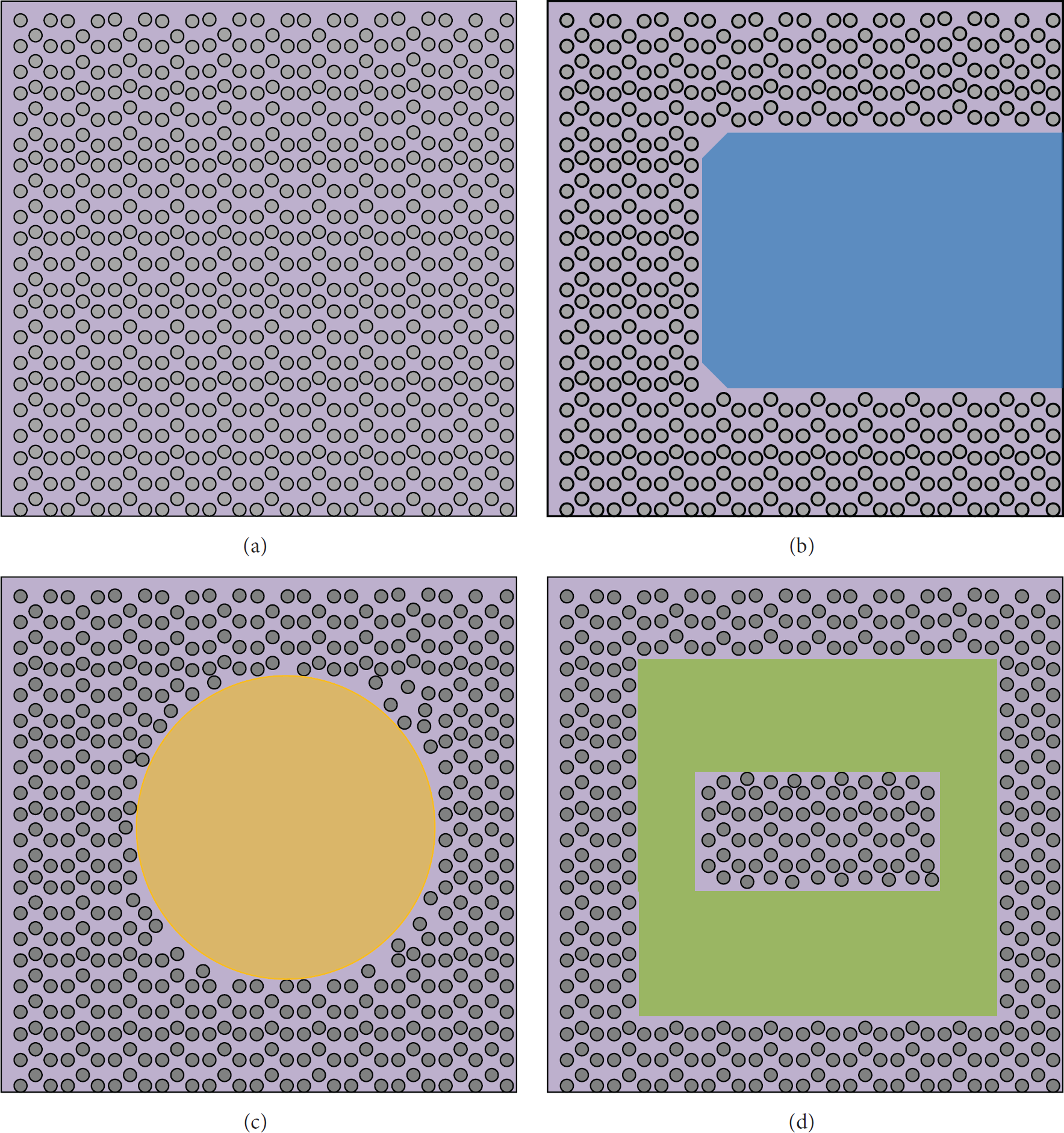
For the first type, according to whether there exist hollows and the shape of the hollows, the network can be simply classified into four simple shapes, as shown in Figure 4. The values of the degree of anisotropy of different topology networks are obtained through experiments and the results are as Table 2 shows.

Table 2

The results of the degree of anisotropy for different topology.

Topology	The value of the degree of anisotropy $D_{\text{node}}$
Uniform	0
C	138.24
O	54.20
8	41.05

Figure 4

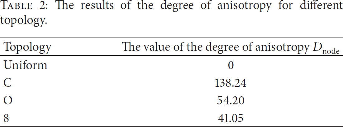
Different topologies with hollows in the network. The lengths of a side for four regions are all 500 m, and there are 600 nodes in the region. (a) is even distribution; (b) is “C” topology; (c) is “O” topology; and (d) is “8” topology.

We can see from Table 2 that the value of the degree of anisotropy in “C” topology of network is the greatest and is much more greater than the value of the remaining three topologies. The second is “O” topology and the third is “8” topology. The value of the degree of anisotropy is 0 when the nodes in the whole network are distributed uniformly. Comparing with “C” topology, the “O” topology is symmetrical and the symmetry is up and down, while the size of hollow in “8” topology is relatively smaller and the symmetry is much more stronger, which is left and right and up and down. We analyzed the results of the model and it turned out to be consistent with the facts; thus the model is feasible.

As for the second type, according to the difference among nodes density in each subregion, the network can be simply classified into four examples, as shown in Figure 5, and the nodes density is gradually greater from left to right and up to down.

Figure 5

Different topologies with different nodes density in each subregion (the density is gradually greater from left to right, up to down). The lengths of a side for four regions are all 500 m, and there are 600 nodes in the region. And the nodes density in (a) is 6.5 : 3.5, in (b) is 8 : 2, in (c) is 1 : 2 : 4 : 3, and in (d) is 0.5 : 1.5 : 2 : 6.

The experiment results of the degree of anisotropy for four topology networks are as Table 3 shows. We can see from Table 3 that when the network is divided into four subregions, where the nodes density in four subregions is 0.5 : 1.5 : 2 : 6, the degree of anisotropy is the biggest. The second is the two subregions where the nodes density is 8 : 2. The third is four subregions where the nodes density is 1 : 2 : 4 : 3, and the least is the two subregions where the nodes density is 6.5 : 3.5. The results are consistent with the facts through analysis; thus the model is feasible.

Table 3

The results of the degree of anisotropy of different topology.

Topology	The value of the degree of anisotropy $D_{\text{node}}$
6.5 : 3.5	37.82
8 : 2	119.53
1 : 2 : 4 : 3	61.10
0.5 : 1.5 : 2 : 6	213.85

Comparing the network where the nodes distribution is uniform and there exist hollows with the network where the nodes distribution is nonuniform and there exist no hollows, we know that the degree of anisotropy for the network where nodes density is not the same in each subregion is much more bigger than that for the network where nodes density is uniform in the whole network. That is because, for the network where there exist hollows, the difference of nodes density is only local while, for the network that the nodes density is different in each subregion, the difference of nodes density is global.

4. Subregional Division

In anisotropy network, nodes density in the whole network is different. So in order to obtain a node's accurate position, the network needs to be divided into many subregions where the nodes density is relatively uniform. In this section, we introduce a method to divide the network automatically, and the division is done according to the number of neighbors and RSSI sequence of neighbors.

4.1. Subregional Division according to the Number of Neighbor Nodes

In this section, actual deployments and simulation experiments are done to do subregional division according to the number of neighbors. The actual deployment is shown in Figure 6 and the simulation topology is shown in Figure 7. In actual deployment, the size of the network was 24 × 24 m², there were 16 Micaz nodes deployed totally, and the network was divided into four subregions according to the nodes density. The sending power of nodes is set −10 dBm, the communication range is about 12 m, and each node broadcasts a packet every 5 seconds. If a node can receive the packet from another node, the two nodes can be thought as neighbors, and the number of neighbor nodes for each node in each subregion is recorded.

Figure 6

The deployment in actual environment.

Figure 7

The simulation topology of the network.

As shown in Figure 8, the numbers of neighbors in areas 1, 2, 3, and 4 are different. Ideally, the number of neighbors in area 1 where nodes density is the most intensive is between 10 and 13, while in area 2 it is between 6 and 8, in area 3 it is between 4 and 6, and in area 4 it is about 12. We can see from Figure 8 that the numbers of neighbors are different in different areas. Therefore, using the number of neighbors to divide the network is feasible.

Figure 8

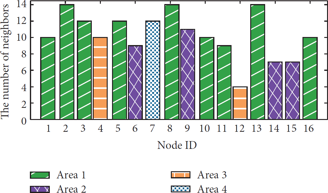
The number of neighbors in different areas.

However, in actual deployment, the number of deployed nodes is limited. In some areas, the number of nodes is too few and it cannot reflect the number of neighbors effectively. Based on that, the experiments need to be done in simulation topology, and Table 4 shows the parameters of simulation topology.

Table 4

The parameters of simulation environment.

Parameters setting	Descriptions
Size	500 × 500 (m2)
Node count	200, randomly distributed
Communication range	100 m

As shown in Table 4, in simulation experiments, the size of the area was 500 × 500 m²; there were 200 nodes randomly distributed in the area and the communication range of nodes was 100 m. The experiments are run 50 times and the number of neighbors for each node is recorded and its mean value is calculated. Here, the effect of beacon nodes is not considered, and the results are shown in Figure 9.

Figure 9

The number of neighbors in the whole network.

We can see from Figure 9 that when the communication range is fixed and the nodes in the network are uniformly distributed, the number of neighbors follows Gaussian distributions and it fluctuates in a small range. Therefore, the number of neighbors can reflect the nodes density in the network effectively, and it can be used to divide the network.

The results of actual deployments and simulation experiments show that when the size of the network and the nodes' positions are fixed, the number of neighbors of each node can reflect the topology of the network effectively; thus it can be used to divide the network.

4.2. Subregional Division according to the RSSI Sequence of Neighbors

However, using the number of neighbors to divide the network is not enough. As shown in Figure 9, how to process the abnormal data is still a problem. Besides, using the number of neighbors can reconstruct the network logically. However, the logical topology is different from the physical topology.

As shown in Figure 6, there is only node $v_{\mathrm{7}}$ deployed in area 4. If the communication range of the node is 12 m, the neighbors of $v_{\mathrm{7}}$ node are $v_{\mathrm{3}}$ , $v_{\mathrm{4}}$ , $v_{\mathrm{10}}$ , $v_{\mathrm{12}}$ , $v_{\mathrm{13}}$ , and $v_{\mathrm{16}}$ in ideal condition, and the distances between $v_{\mathrm{7}}$ node and them are separately 9.5 m, 6 m, 12 m, 12 m, 9.5 m, and 9 m. However, in actual cases, the neighbors' number of $v_{\mathrm{7}}$ node is 12 according to the collected information. Therefore, only using the number of neighbors cannot divide the network effectively.

Based on that, a better way needs to be considered to divide the network effectively. RSSI value is another information that can be obtained. Although RSSI is easily affected by environmental distance and it cannot reflect the precise distance between nodes, from the view of coarseness, RSSI can reflect whether a node is near to or far away from another node. Therefore, RSSI information can be used to correct the number of neighbors; then the corrected number of neighbors is used to divide the network.

RSSI values of neighbors have a certain stable range for each node. When the RSSI value between two nodes is below the certain range, they can be seen far away from each other, and the node can be seen as a noise point and it can be removed from the neighbors and the neighbors' number reduces by 1.

4.3. Subregional Division according to the Number of Neighbors and RSSI Sequence of Neighbors

Before introducing the steps, some descriptions of nouns will be given.

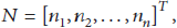
When given the number of nodes n, the neighbors' number of all the nodes can be expressed by vector N:

$$\begin{array}{cc}& N={\left[n_{\mathrm{1}},n_{\mathrm{2}},\dots ,n_n\right]}^T,\end{array}$$

(5)

where $n_i$ represents the neighbors' number of node i. As for the RSSI sequence of neighbors of node i, it can be expressed by vector $R_i$ :

$$\begin{array}{cc}& R_i={\left[r_{i\mathrm{1}},r_{i\mathrm{2}},\dots ,r_{im}\right]}^T,\end{array}$$

(6)

where $r_{ij}$ is the RSSI value between node i and node j. The RSSI values of neighbors of all nodes in the whole network can be expressed by matrix R:

$$\begin{array}{cc}& R=\left[R_{\mathrm{1}},R_{\mathrm{2}},\dots ,R_n\right],\end{array}$$

(7)

where the ith row of the matrix represents the RSSI sequence of neighbors of node i.

Then the specific steps will be given and they are as follows.

• (1)

Correct the number of neighbors according to RSSI sequence of neighbors.

  

Firstly, RSSI values of neighbors are used to correct the number of neighbors, and the node where RSSI value is more than or less than a certain range will be removed from the neighbors. That can be done according to the following equation:

$$\begin{array}{cc}& g_i=\frac{r_{ij}-E\left(R_i\right)}{E\left(R_i\right)},\hspace{1em}{r}_{ij}=\left\{\begin{array}{cc}\mathrm{1},\hfill & g_i⩽t_n,\hfill \\ \mathrm{0},\hfill & g_i>t_n,\hfill \end{array}\right.\end{array}$$

(8)

where $E(R_i)=\left(\mathrm{1}/n_i\right){\sum }_{j=\mathrm{1}}^{n_i}‍r_{ij}$ , $t_n$ is the threshold value of neighbors' number, and $E(R_i)$ is the mean value of all neighbors' RSSI values of node i. If $r_{ij}=\mathrm{0}$ , the node j will be removed from the neighbors of node i, and the number of neighbors of node i is minus 1.

(2)

Divide the network using the corrected number of neighbors.

  

Based on that, vector N of the whole network needs to be updated and an updated vector is expressed by $N^{\prime }$ :

$$\begin{array}{cc}& N^{\prime }={\left[n_{\mathrm{1}}^{\prime },n_{\mathrm{2}}^{\prime },\dots ,n_n^{\prime }\right]}^T.\end{array}$$

(9)

The numbers of neighbors of node i and node j are computed as the following equation:

$$\begin{array}{cc}& \begin{array}{cc}\left|n_i^{\prime }-n_j^{\prime }\right|⩽t_r,& \forall v_i,v_j\in G,\\ \mathrm{o}\mathrm{t}\mathrm{h}\mathrm{e}\mathrm{r}\mathrm{w}\mathrm{i}\mathrm{s}\mathrm{e},& \forall v_i,v_j\notin G,\end{array}\end{array}$$

(10)

where $t_r$ represents the threshold value of the difference of neighbors' number. If the difference of corrected neighbors' number is less than the threshold value, the density of the two nodes can be seen as similar, and they belong to the same density area. Otherwise, they do not belong to the same density area.

5. Node Density-Based Subregional Localization Algorithm

There have been many methods proposed to solve the nodes localization problem in anisotropy network, led by REP algorithm [14] proposed by Li and Liu, LAEP algorithm [29] proposed by Wang et al., and PDM algorithm proposed by Lim and Hou [30]. However, the proposed algorithms are feasible theoretically and they are hard to apply to real environment. Besides, they are feasible in small scale anisotropy network, such as in a room or in a small building; there will exist some challenges when they are applied to large scale anisotropy network.

We propose a node density-based subregional localization algorithm. The algorithm is divided into four steps, as shown in Figure 10, and they are boundary detection, regional division, distance measurement, and nodes localization.

Figure 10

The overview of NDSL algorithm.

5.1. Boundary Detection

The neighbors' number of boundary node is usually small and when it is used to divide the network, there will exist error. So before regional division, the boundary nodes need to be preprocessed.

There are two kinds of algorithms for boundary detection: one is based on geometrical topology and another is based on statistical thoughts. Wang et al. [33] proposed an algorithm to detect the boundary nodes by constructing a tree of shortest path of the network, and there is no requirements for the network topology itself in the algorithm. Thus it can be used in this paper to detect the boundary nodes in anisotropy network. After the boundary detection of the network, the nodes of the network will be divided into two parts: they are boundary nodes and nonboundary nodes, which are represented separately as $V_{\mathrm{e}\mathrm{d}\mathrm{g}\mathrm{e}}=\{v_e^{\mathrm{1}},v_e^{\mathrm{2}},\dots ,v_e^m\}$ and $V_{\mathrm{n}\mathrm{o}\mathrm{r}\mathrm{m}}=\{v_r^{\mathrm{1}},v_r^{\mathrm{2}},\dots ,v_r^{n-m}\}$ .

5.2. Regional Division

Regional division is the most important step in NDSL algorithm, and, in this paper, the network is divided according to the number of neighbors, which is in the range of single-hop distance and the RSSI sequence of neighbors. The details are already introduced above (Section 4.3). After regional division, the network is divided into many subregions where the nodes density is relatively uniform. Comparing with other algorithms, NDSL algorithm solves the nodes localization problem in large scale anisotropy network and the main steps for regional division are as follows.

(i) Topology Discovery. The network needs to be initialized for NDSL algorithm, and the topology discovery is achieved by broadcast data; then the number of neighbors and RSSI sequence of neighbors for each node will be obtained.

(ii) Regional Division for Nonboundary Nodes. After initialization, the network will be divided. Considering the difference of neighbors' number between boundary nodes and nonboundary nodes, the regional division is only done for nonboundary nodes $V_{\mathrm{n}\mathrm{o}\mathrm{r}\mathrm{m}}$ . First, beacon nodes send data packets of regional division to their neighbor nodes, and when the neighbor nodes receive the data packets, they will decide whether they are in the same subregion according to the number of neighbors and the RSSI sequence of neighbors. If the node meets the requirements of regional division, it will send data packets to its neighbor nodes to decide whether its neighbor nodes meet the requirements. If the node does not meet the requirement of regional division, the node will be as the center node to redo the above steps. That is an iterative process until the nodes' density in each subregion is relatively uniform.

(iii) Regional Division for Boundary Nodes. On the basis of the regional division above, a special division will be done for the boundary nodes. For boundary nodes, there will be many nonboundary neighbor nodes, and, among those nonboundary neighbor nodes, there will exist a nonboundary neighbor node where the number of neighbors is the most. Then the boundary node will be thought to belong to the subregion in which that nonboundary neighbor node is in.

5.3. Distance Calculation

In this paper, an improvement is done for DV-Hop algorithm; however, different from DV-Hop algorithm, NDSL algorithm locates the nodes using regional division and computes different single-hop distance for different subregions; thus the localization accuracy improves.

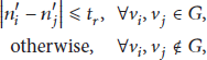
Assume that the single-hop distance for subregion 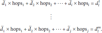$A_i$ is ${\tilde{d}}_i$ ; there are m links among beacon nodes in the network; the actual distance for each link is $d_l^m$ ; then we will count which subregion beacon nodes passed and also count the hop counts $\mathrm{h}\mathrm{o}\mathrm{p}{\mathrm{s}}_i$ in each subregion. The single-hop distance for each subregion is optimized by the following equation:

$$\begin{array}{cc}& {\tilde{d}}_{\mathrm{1}}\times \mathrm{h}\mathrm{o}\mathrm{p}{\mathrm{s}}_{\mathrm{1}}+{\tilde{d}}_{\mathrm{2}}\times \mathrm{h}\mathrm{o}\mathrm{p}{\mathrm{s}}_{\mathrm{2}}+\cdots +{\tilde{d}}_i\times \mathrm{h}\mathrm{o}\mathrm{p}{\mathrm{s}}_i=d_l^{\mathrm{1}}\\ ⋮\\ {\tilde{d}}_{\mathrm{1}}\times \mathrm{h}\mathrm{o}\mathrm{p}{\mathrm{s}}_{\mathrm{1}}+{\tilde{d}}_{\mathrm{2}}\times \mathrm{h}\mathrm{o}\mathrm{p}{\mathrm{s}}_{\mathrm{2}}+\cdots +{\tilde{d}}_j\times \mathrm{h}\mathrm{o}\mathrm{p}{\mathrm{s}}_j=d_l^m.\end{array}$$

(11)

For those regions which the links of beacon nodes do not cover, the single-hop distance of the region can be seen as the single-hop distance of the nearest beacon node.

5.4. Nodes Localization

When the single-hop distance of each subregion is obtained, the distance $\mathrm{d}\mathrm{i}\mathrm{s}{\mathrm{t}}_i$ between unknown node and beacon node i is estimated according to the following equation:

$$\begin{array}{cc}& \mathrm{d}\mathrm{i}\mathrm{s}{\mathrm{t}}_i={\displaystyle \sum }_{t=\mathrm{1}}^k\left({\tilde{d}}_t\times \mathrm{h}\mathrm{o}\mathrm{p}{\mathrm{s}}_t\right).\end{array}$$

(12)

When three or more than three distances from beacon nodes are obtained, the least square method [9] is used to estimate the position of unknown node.

6. Test-Based Results

In this part, we will experiment in actual deployments to evaluate NDSL algorithm, and the deployments are separately linear network and rectangle 2D network, and Figure 11 is the scenario of actual deployment.

Figure 11

The true deployment in our campus.

6.1. Linear Network

The evaluation starts from a linear network, which is the most simple network topology.

(1) Experiment Setup. As shown in Figure 12, there were 16 Micaz nodes deployed for linear network. The network was divided into three sections, and the distance between nodes in area 1 was 0.8 m, in area 2 it was 1.6 m, and in area 3 it was 2.4 m. Each Micaz node was left 80 cm above the ground in order to reduce the absorption of the signals. Each node broadcasted a packet every 30 s and the sending power was set −10 dBm.

Figure 12

Experiment setup of linear network.

(2) Localization Performance. As shown in Table 5, in linear network, the maximum distance between nodes is 56.5 m, and the max hops in the network are 4 hops when the single-hop distance is 13 m. Table 5 shows that the average numbers of neighbor nodes in area 1, area 2, and area 3 are separately 7.4, 9, and 4.8. Figure 13 shows the number of neighbors before and after selection; we can see from Figure 13 that after selection, the distribution of the neighbors' number is more regular, and node 1 and node 10 remove many neighbor nodes that do not meet the requirements of regional division.

Table 5

Statistics of the linear network.

Scale	Hops max	Single hop	Neighborhood
			1	2	3
≈56.5 m	4	≈13 m	7.4	9	4.8

Figure 13

Comparison of neighbors' number between raw and after selection in linear network.

In this paper, we define localization error as follows:

$$\begin{array}{cc}& \mathrm{E}\mathrm{r}\mathrm{r}\mathrm{o}{\mathrm{r}}_p=\frac{\sqrt{{\left(x_e-x_t\right)}^{\mathrm{2}}-{\left(y_e-y_t\right)}^{\mathrm{2}}}}{R},\end{array}$$

(13)

where $\left\{x_e,y_e\right\}$ , $\left\{x_t,y_t\right\}$ represent separately the node's estimate position and the node's actual position while R represents the communication range of nodes.

Figure 14 shows the localization error of linear network when using DV-Hop algorithm and NDSL algorithm separately. We can see from Figure 14 that NDSL algorithm is superior to DV-Hop algorithm in linear network, and for those nodes, where the localization error of DV-Hop is very big, such as nodes 4, 8, and 10, NDSL algorithm can improve its accuracy effectively.

Figure 14

Comparison of localization accuracy between DV-Hop algorithm and NDSL algorithm in linear network.

6.2. Rectangle 2D Network

(1) Experiment Setup. The experiment setup is almost the same as linear network, and the difference is that there were 35 Micaz nodes deployed in the network, as shown in Figure 15.

Figure 15

Experiment setup of rectangle 2D network.

(2) Localization Performance. As shown in Table 6, in rectangle 2D network, there are 60 pairs of nodes in single hop, 54 pairs of nodes in two hops, and 10 pairs of nodes in three hops. Figure 16 shows the number of neighbors before and after selection; we can see from Figure 16 that, after selection, the distribution of the neighbors' number is more regular.

Table 6

Statistics of the rectangle 2D network.

Statistics	1 hop	2 hops	3 hops
Number	60	54	10
Min distance	4.2	6.2642	25.0567
Median distance	10.751	19.4854	29.3372
Max distance	15.7124	32.4222	37.819

Figure 16

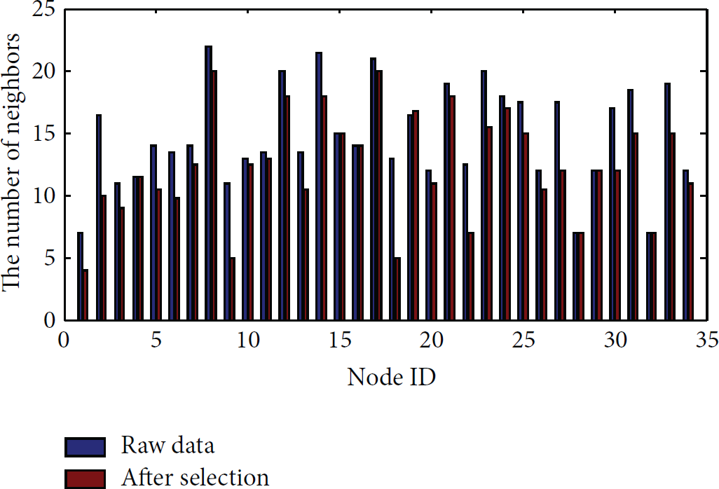
Comparison of neighbors' number between raw and after selection in rectangle network.

Figure 17 shows the localization error of rectangle 2D network when using DV-Hop algorithm and NDSL algorithm separately. In order to eliminate the effect of beacon nodes on localization results, we choose 30 nodes randomly to do localization, and the error is ranked from big to small. We can see from Figure 17 that NDSL algorithm is superior to DV-Hop algorithm in rectangle 2D network.

Figure 17

Comparison of localization accuracy between DV-Hop algorithm and NDSL algorithm in rectangle network.

Test-bed experiments show that NDSL provides better accuracy than DV-Hop algorithm in anisotropy network.

Through analysis of max error, mean error, and min error, as shown in Figure 18, and combining with the degree of anisotropy of the two types of network, we know that

• (1)

NDSL improves accuracy obviously in two types of networks compared with DV-Hop algorithm;

(2)

from the view of max error, mean error, and min error, the accuracy of NDSL algorithm improves more obviously in rectangle 2D network than linear network;

(3)

comparing with small error, NDSL algorithm decreases big error obviously.

Figure 18

Comparison of localization error between linear network and rectangle 2D network.

7. Simulation Experiment

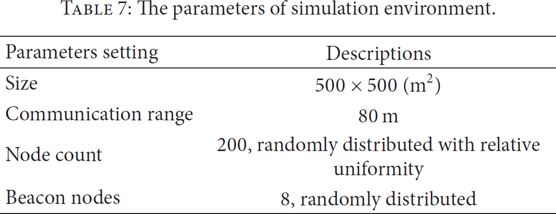
In simulation experiments, two types of networks are done and they are separately rectangle network where no hollows exist and C network where a hollow exists, as shown in Figure 19. Table 7 shows the parameters of simulation network, and all the experiments are run 30 times and then the mean value is calculated. When the size of area and the topology of the network are determined, the change of communication range will influence the number of neighbors and the number of beacon nodes will also influence the accuracy of localization.

Table 7

The parameters of simulation environment.

Parameters setting	Descriptions
Size	500 × 500 (m2)
Communication range	80 m
Node count	200, randomly distributed with relative uniformity
Beacon nodes	8, randomly distributed

Figure 19

Two types of simulation network.

7.1. The Changes of Communication Range

We know that when the distribution of the network is fixed, the change of communication range will directly influence the number of neighbors. The bigger the communication range, the more the nodes that can be covered, and the hop counts of the network decrease. That will lead to the decrease of measurement error.

As shown in Figure 20(a), when the communication range changes from 80 m to 125 m, NDSL algorithm works better than DV-Hop algorithm. The results show the following.

• (1)

When the communication range is the same, NDSL algorithm performs better compared with DV-Hop algorithm. In rectangle network, the localization accuracy improves 9% most, while in C network, the localization accuracy improves 25% most.

(2)

With the increase of communication range, the localization accuracy of two methods all increases. However, the increasement of NDSL algorithm is higher than DV-Hop algorithm.

Figure 20

Comparison between DV-Hop algorithm and NDSL algorithm.

7.2. The Changes of Beacon Nodes

When the number of beacon nodes in the network becomes greater, the more localization information can be obtained from beacon nodes, and the localization accuracy will be improved accordingly. In simulation experiments, the experiments are run when the number of beacon nodes changes from 3 to 14. As shown in Figure 20(b), when the number of beacon nodes increases, NDSL algorithm works better than DV-Hop algorithm. The results show the following.

• (1)

When the number of beacon nodes is the same, NDSL algorithm performs better compared with DV-Hop algorithm. In rectangle network, the localization accuracy improves 10% most, while in C network, the localization accuracy improves 40% most.

(2)

With the increase of the number of beacon nodes, the localization accuracy of two methods all increases. However, the increasement of NDSL algorithm is higher than DV-Hop algorithm.

(3)

With the increase of the number of beacon nodes, the localization error decreases. When the number of beacon nodes is 9, the increasement of accuracy will not be obvious with the increase of the number of beacon nodes, especially in rectangle network.

7.3. Error

The error comes from many aspects, such as the measurement error of nodes, the position error of beacon nodes, and the calculation error of localization results. The reasons that caused error are various, for example, disturbance of environment on signal, the difference of nodes itself, and network topology. In anisotropy network, most of the error comes from ranging error; thus the performance of NDSL algorithm also needs to be considered from the view of ranging error.

Figure 21 shows the ranging error and localization error in simulation rectangle network when using DV-Hop algorithm and NDSL algorithm and we can see from Figure 21 that NDSL algorithm is superior to DV-Hop algorithm no matter in ranging error or localization error. The results show the following.

• (1)

In ranging error, NDSL algorithm works better than DV-Hop algorithm in big error, as shown in Figure 21(a); NDSL algorithm improves the ranging error most from 20 m to 60 m. That is because when a node is near to another node, the hop counts between the two nodes are small; thus the cumulative error that is caused by the single-hop distance of DV-Hop algorithm is not obvious. When a node is far away from another node, the cumulative error is significantly larger.

(2)

In localization error, NDSL algorithm works better than DV-Hop algorithm. In simulation network, for NDSL algorithm, 80% of the localization error is within 40 m while, for DV-Hop algorithm, the percent is just 65%.

Figure 21

Comparison of ranging error and localization error between DV-Hop algorithm and NDSL algorithm.

8. Conclusion

We presented NDSL, a node density-based subregional localization method in large scale anisotropy network. Different from DV-Hop algorithm, NDSL algorithm divided the network into many subregions according to the number of neighbors and RSSI sequence of neighbors. Then NDSL algorithm corrected single-hop algorithm of each subregion to improve accuracy. Besides, we also proposed a model to evaluate the degree of anisotropy of anisotropy network. Experiment results demonstrated that the model was feasible. Through actual deployment and simulation experiments, the results showed that NDSL algorithm can improve the localization accuracy effectively compared with DV-Hop algorithm.