Decomposition Based Localization for Anisotropic Sensor Networks

Abstract

Range-free localization algorithms have caused widespread attention due to their low cost and low power consumption. However, such schemes heavily depend on the assumption that the hop count distance between two nodes correlates well with their Euclidean distance, which will be satisfied only in isotropic networks. When the network is anisotropic, holes or obstacles will lead to the estimated distance between nodes deviating from their Euclidean distance, causing a serious decline in localization accuracy. This paper develops HCD-DV-Hop for node localization in anisotropic sensor networks. HCD-DV-Hop consists of two steps. Firstly, an anisotropic network is decomposed into several different isotropic subnetworks, by using the proposed Hop Count Based Decomposition (HCD) scheme. Secondly, DV-Hop algorithm is carried out in each subnetwork for node localization. HCD first uses concave/convex node recognition algorithm and cleansing criterion to obtain the optimal concave and convex nodes based on boundary recognition, followed by segmentation of the network's boundary. Finally, the neighboring boundary nodes of the optimal concave nodes flood the network with decomposition messages; thus, an anisotropic network is decomposed. Extensive simulations demonstrated that, compared with range-free DV-Hop algorithm, HCD-DV-Hop can effectively reduce localization error in anisotropic networks without increasing the complexity of the algorithm.

1. Introduction

Node localization is one of the most fundamental technologies in wireless sensor networks (WSNs). For most applications of WSNs [1–3], only when nodes know their locations can they tell the system “what is happening in what position.” For instance, in a fire monitoring system, a sensor node detects that a fire breaks out. The system is able to notify people where the fire is only when it knows the node's location. This allows fireman to reach the correct location and take effective measures immediately in order to prevent the spread of the fire. In addition, accurate localization is the foundation of many other WSNs technologies, such as position-aware data processing [4–6] and geographic routing [7, 8].

Among existing localization algorithms, range-free schemes [9–12] have been widely used due to their low cost and low power consumption. However, these schemes assume that the hop count distance between two nodes correlates well with their Euclidean distance, which will be satisfied only in isotropic networks [9, 13] (the definition of isotropic and anisotropic networks can be found in [14]). In practical applications, such as large-scale heritage protection [15] and military reconnaissance [16], sensor nodes are often randomly deployed in complex environments, which makes their network topologies highly irregular, with the possibility of holes or obstacles. Such network is called anisotropic network.

For example, Figure 1 shows an application of WSNs. In this scenario, sensors are distributed in the region to be monitored, and Figure 2 shows the corresponding node deployment. It is obvious in Figure 2 that the hop count distances between some pairs of nodes heavily deviate from their Euclidean distances (Take A and B in Figure 2, e.g., the black solid line represents the hop count distance between A and B, and the orange dotted line represents the Euclidean distance between them). Using the deviated shortest path distance instead of Euclidean distance to take part in localization will cause a serious decline in localization accuracy.

Figure 1

Application example of WSNs.

Figure 2

Node deployment.

(1) Related Work. In order to improve the node localization accuracy in anisotropic networks, scholars have put forward many schemes in recent years, which can be divided into three categories.

The first scheme is mainly dedicated to amending the estimated distance between nodes. Li and Liu [17] proposed REP (Rendered Path) for localization in anisotropic sensor networks. REP assumes that the boundary nodes around obstacles have been obtained by a boundary recognition algorithm. The shortest path between nodes is divided into many different subsections according to the location of the obstacles. The angle between two subsections is calculated by constructing a unit circle in the intersection point of the shortest path and network holes; then, the Euclidean distance can be obtained by using the cosine law. REP is able to amend the estimated distance that is affected by obstacles. The main drawback is that REP suffers heavy computation and communication overhead, requiring high density and computation power of nodes. PDM (Proximity-Distance Map) [18] first uses a matrix to record the estimated distance and the Euclidean distance between anchor nodes. Then, it calculates the linear transformation matrix between the estimated distance and the Euclidean distance using the least square method. By using the linear transformation matrix, the estimated distance can be transformed into an amended distance, which is used to participate in localization. The disadvantage is that PDM requires the uniform deployment of anchor nodes, which is difficult in real applications.

The second solution aims at reducing the localization error by avoiding serious bent path participating in localization. Reference [19] proposed an improvement scheme for DV-Hop. It uses the cubic polynomial interpolation to obtain paths that are not heavily bent. By using these “good” paths in the calculations, the performance of DV-Hop in an anisotropic network can be improved. Reference [20] estimates the shortest paths affected by obstacles or network boundaries between unknown nodes and anchor nodes. By grading the estimating result, [20] chooses the anchor nodes corresponding to those less affected paths to participate in calculation, thus reducing the localization error. Reference [21] chooses some suitable anchor nodes in the networks and calculates the locations of unknown nodes through iterative multilateration. The localization error is controlled by avoiding the use of serious bent paths. Since iterative multilateration is employed, there is cumulative effect in localization error. Reference [22] proposed an improved multihop localization algorithm which is called i-multihop. It can automatically identify and eliminate severely miscalculated distances. In the localization process, these “bad” distances will not be used in calculation. Thus, the localization error can be controlled.

The third method achieves localization of unknown nodes by means of building landmark network. Reference [23] first locates a landmark network, which is composed of nodes that are uniformly sampled from the original network. The density of the landmark network is preset by the system. Each nonlandmark node uses trilateration to calculate its own location according to the distances to its closest three landmarks. References [24, 25] first select some landmark nodes using particular rules. Then, they calculate the Voronoi diagram and its dual Delaunay diagram according to the landmark nodes. The location of an unknown node is computed in each subdiagram. Finally, the original network can be restored through all the Delaunay diagrams. The difference between [24] and [25] is the method of selecting landmarks. Since both of the algorithms require Delaunay division for anisotropic networks, they are much more complicated to implement, which limits the application of the algorithms.

As can be seen from the above analysis, the similarity among the methods in [17–22] is that they all use various mechanisms to avoid or amend serious bent paths, which does not fundamentally solve the impact of anisotropic networks characteristics on localization. Although the schemes in [24, 25] proposed new ideas, their implementation processes are complex, which is not suitable for large-scale sensor networks.

(2) The HCD-DV-Hop Scheme. In this paper, a new method for localization is proposed based on decomposition. Our scheme is composed of two steps. First, it decomposes an anisotropic network into several isotropic subnetworks by using the proposed Hop Count Based Decomposition (HCD) algorithm. Second, it uses the typical range-free DV-Hop algorithm to achieve node localization in each subnetwork. For simplicity, we call the proposed method HCD-DV-Hop algorithm. The contributions of this paper are summarized as follows:

• (i)

We analyze the reason why range-free DV-Hop algorithm is suitable for localization in isotropic networks but causes serious localization error in anisotropic networks. Then, we give an improved solution.

(ii)

We introduce a distributed localization algorithm for anisotropic networks, which is called HCD-DV-Hop algorithm. HCD-DV-Hop first decomposes an anisotropic network into several different isotropic networks, so that the influence of holes or obstacles on the shortest communication path between far-away nodes is avoided. Since there is no longer serious bent path in each isotropic subnetwork, DV-Hop can be carried out for node localization in such subnetwork.

(iii)

A Hop Count Based Decomposition (HCD) algorithm for anisotropic networks is proposed. HCD includes four steps: boundary recognition, concave/convex node recognition and cleansing, boundary segmentation, and region decomposition. All of these steps are distributed and only require connectivity information.

(iv)

Simulation results demonstrate the superior performance of HCD-DV-Hop under different ratios of anchor node and communication radius in anisotropic networks.

The rest of this paper is organized as follows. In Section 2, we present the motivation of our scheme. Section 3 is an overview of HCD-DV-Hop. Section 4 is devoted to a description of the proposed HCD algorithm for anisotropic networks. The performance of HCD-DV-Hop is evaluated in Section 5. Finally, Section 6 concludes this paper.

2. Motivation

2.1. DV-Hop Algorithm

DV-Hop [9, 26] is one of the most widely used range-free schemes and it consists of three steps.

Step 1 (obtain the minimum hop count).

Each anchor node broadcasts its location information and hop count value with a packet $(x_i,y_i,h_i)$ , where $(x_i,y_i)$ is the coordinate of anchor node i and $h_i$ is the minimum hop count from the anchor node i. By this means, all nodes (including anchor and unknown nodes) can obtain locations of anchor nodes and minimum hop count to each anchor.

Step 2 (calculate the estimated distance).

Once an anchor node gets distances to other anchors, it estimates an average size for one hop, that is, $C_i$ , which is then deployed as a correction to the entire network:

$$\begin{array}{cc}& C_i=\frac{{\sum }_{j\ne i}\sqrt{{\left(x_i-x_j\right)}^{\mathrm{2}}+{\left(y_i-y_j\right)}^{\mathrm{2}}}}{{\sum }_{j\ne i}{h}_i},\end{array}$$

(1)

where $(x_i,y_i)$ and $(x_j,y_j)$ are the coordinates of anchor node i and anchor node j and $h_i$ is the minimum hop count between anchor nodes i and j. Each unknown node receives the correction from its nearest anchor node and multiplies it by the minimum hop count, so that the estimated distance to each anchor node is obtained.

Step 3 (each unknown node estimates its location by using the maximum likelihood estimation).

Let the coordinate of unknown node M be $(x,y)$ , and the distance between anchor node i and unknown node M is $d_i$ . Assuming there are n anchor nodes in the network, (2) can be obtained:

$$\begin{array}{cc}& {\left(x-x_{\mathrm{1}}\right)}^{\mathrm{2}}+{\left(y-y_{\mathrm{1}}\right)}^{\mathrm{2}}=d_{\mathrm{1}}^{\mathrm{2}},\\ {\left(x-x_{\mathrm{2}}\right)}^{\mathrm{2}}+{\left(y-y_{\mathrm{2}}\right)}^{\mathrm{2}}=d_{\mathrm{2}}^{\mathrm{2}},\\ ⋮\\ {\left(x-x_n\right)}^{\mathrm{2}}+{\left(y-y_n\right)}^{\mathrm{2}}=d_n^{\mathrm{2}}.\end{array}$$

(2)

By using the maximum likelihood estimation, we get the location of unknown node M by

$$\begin{array}{cc}& X={\left(A^{\prime }A\right)}^{-\mathrm{1}}{A}^{\prime }B,\end{array}$$

(3)

where

$$\begin{array}{cc}& A=\left[\begin{array}{cc}\mathrm{2}\left(x_{\mathrm{1}}-x_n\right)& \mathrm{2}\left(y_{\mathrm{1}}-y_n\right)\\ \mathrm{2}\left(x_{\mathrm{2}}-x_n\right)& \mathrm{2}\left(y_{\mathrm{2}}-y_n\right)\\ ⋮& ⋮\\ \mathrm{2}\left(x_{n-\mathrm{1}}-x_n\right)& \mathrm{2}\left(y_{n-\mathrm{1}}-y_n\right)\end{array}\right],\\ B=\left[\begin{array}{c}{x}_{\mathrm{1}}^{\mathrm{2}}+y_{\mathrm{1}}^{\mathrm{2}}-x_n^{\mathrm{2}}-y_n^{\mathrm{2}}+d_n^{\mathrm{2}}-d_{\mathrm{1}}^{\mathrm{2}}\\ x_{\mathrm{2}}^{\mathrm{2}}+y_{\mathrm{2}}^{\mathrm{2}}-x_n^{\mathrm{2}}-y_n^{\mathrm{2}}+d_n^{\mathrm{2}}-d_{\mathrm{2}}^{\mathrm{2}}\\ ⋮\\ x_{n-\mathrm{1}}^{\mathrm{2}}+y_{n-\mathrm{1}}^{\mathrm{2}}-x_n^{\mathrm{2}}-y_n^{\mathrm{2}}+d_n^{\mathrm{2}}-d_{n-\mathrm{1}}^{\mathrm{2}}\end{array}\right],\\ X=\left[\begin{array}{c}x\\ y\end{array}\right].\end{array}$$

(4)

2.2. The Limitation of DV-Hop in Anisotropic Networks

As can be seen from DV-Hop, the estimated location accuracy of an unknown node depends on the accuracy of its estimated distances to the anchor nodes. That is, if the estimated distance between two nodes is closer to their Euclidean distance, the localization result will be more accurate. If the estimated distance heavily deviates from the Euclidean distance, the localization accuracy will be seriously declined.

In Figure 3, we use $‖AG‖$ and $‖MN‖$ to, respectively, represent the Euclidean distance between nodes A and G and M and N (the dotted line in Figures 3(a) and 3(b)). $\left|AG\right|$ and $\left|MN\right|$ are the estimated distances between A and G and M and N, respectively. In DV-Hop, the estimated distance between nodes i and j is calculated by $h_{ij}\times HS$ , where $h_{ij}$ is the minimum hop count between i and j (the hop count represented by the solid line in Figure 3). $HS$ is the average size for one hop. The estimated distance between A and G in Figure 3(a) is

$$\begin{array}{cc}& \left|AG\right|=h_{AG}\times HS\approx ‖AB‖+‖BC‖+‖CD‖+‖DE‖+‖EF‖+‖FG‖.\end{array}$$

(5)

Figure 3

The shortest communication path between nodes in different networks.

The estimated distance between M and N in Figure 3(b) is

$$\begin{array}{cc}& \left|MN\right|=h_{MN}\times HS\approx ‖MH‖+‖HI‖+‖IJ‖+‖JK‖+\cdots +‖KL‖+‖LP‖+‖PQ‖+‖QN‖,\end{array}$$

(6)

where $‖·‖$ represents the Euclidean distance between two nodes. From Figure 3(a), we have

$$\begin{array}{cc}& ‖AB‖+‖BC‖+‖CD‖+‖DE‖+‖EF‖+‖FG‖\approx ‖AG‖.\end{array}$$

(7)

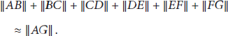
Then,

$$\begin{array}{cc}& \left|AG\right|\approx ‖AG‖.\end{array}$$

(8)

That is to say, the estimated distance between A and G is approximately equal to their Euclidean distance. Therefore, in such isotropic networks, when the estimated distance takes the place of the Euclidean distance in localization, it will not cause serious error. That is why DV-Hop is suitable for localization in isotropic networks.

However, in an anisotropic network like Figure 3(b), it is obvious that

$$\begin{array}{cc}& ‖MH‖+‖HI‖+‖IJ‖+‖JK‖+‖KL‖+‖LP‖+\cdots +‖PQ‖+‖QN‖\gg ‖MN‖.\end{array}$$

(9)

Taking formula (6) into consideration, then we have

$$\begin{array}{cc}& \left|MN\right|\gg ‖MN‖.\end{array}$$

(10)

Formula (10) means that the estimated distance between M and N is much larger than their Euclidean distance. When we use the estimated distance to replace the Euclidean distance to participate in localization, it will cause serious localization error.

From the above analysis, we observe that the shortest communication path between nodes is crucial to localization result. Only when the shortest estimated distance between nodes is approximately equal to their Euclidean distance can the estimated location of node obtained by localization algorithm be approximate to its real location. In an anisotropic network, because of the barrier and irregularity of the network topology, the shortest estimated distance between far-away nodes will heavily deviate from the Euclidean distance, which will cause serious localization error.

A straightforward way is decomposing an anisotropic network into many different isotropic subnetworks and then carrying out DV-Hop for node localization in each subnetwork. Since there is no longer serious bent path between nodes in each subnetwork, the estimated distance can be approximately equal to the Euclidean distance. Therefore, in theory, this scheme can reduce localization error to a certain extent in anisotropic networks.

3. HCD-DV-Hop Overview

In this paper, we assume that the network is fully connected. Our proposed decomposition based localization scheme, that is, HCD-DV-Hop, mainly consists of the following two steps, as is shown in Figure 4.

• (i)

The anisotropic network is decomposed into several different isotropic subnetworks by using the Hop Count Based Decomposition (HCD) algorithm. HCD goes through four steps: boundary recognition, concave/convex node recognition and cleansing, boundary segmentation, and region decomposition, which will be shown in Section 4.

(ii)

For each isotropic subnetwork, the typical range-free DV-Hop algorithm will be carried out for node localization.

Figure 4

HCD-DV-Hop overview.

4. Hop Count Based Decomposition (HCD) Algorithm for Anisotropic Networks

In large-scale wireless sensor networks, there may be thousands of sensor nodes, which makes it almost impossible to decompose the network by artificial means. So this paper will design an algorithm to achieve decomposition by using connectivity information of the network. The proposed Hop Count Based Decomposition (HCD) algorithm consists of four steps.

Step 1 (boundary recognition).

This step aims at recognizing the boundary nodes in the network.

Step 2 (concave/convex node recognition and cleansing).

Based on boundary recognition, the concave/convex node recognition algorithm and cleansing criterion is proposed to obtain the optimal concave and convex nodes.

Step 3 (boundary segmentation).

The optimal concave and convex nodes are used to flood the boundary nodes to segment the boundary into different branches.

Step 4 (region decomposition).

The neighboring boundary nodes of optimal concave nodes flood the network to decompose an anisotropic network into different subnetworks.

4.1. Boundary Recognition

The existing boundary recognition algorithms can be divided into two categories: statistical methods [27] and geometrical methods [28]. After years of researches and developments, scholars have proposed many boundary recognition algorithms with good performance, such as [29–31]. Since this paper mainly focuses on region decomposition and node localization, we directly use [31] in our simulations for boundary recognition.

4.2. Concave/Convex Node Recognition and Cleansing

4.2.1. Definition of Concave/Convex Node Based on Cyclotomy

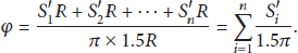
The cyclotomy [32] refers to increasing the number of sides of the regular polygon inside a circle to estimate the circumference by summing them (see Figure 5), based on which the concavity and convexity function of O point is given as

$$\begin{array}{cc}& \phi =\frac{\varphi }{{\mathrm{180}}^{\circ }}\approx \frac{n\times d}{\pi \times R},\end{array}$$

(11)

where d represents side length of the polygon, R is the radius of the circle, and n is the number of sides corresponding to ϕ. It means in (11) that the summation of n sides approximately equals the arc length of ϕ. When the vertexes of the polygon in Figure 5 are regarded as sensor nodes in the network, d can be considered as the maximum communication distance and n is the hop count between nodes.

Figure 5

Schematic diagram of the cyclotomy.

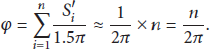
In practical application, since the sensor network is discrete, there may be deviations in the calculation results due to the boundary noise. Considering this factor, the definitions of the concave nodes and the convex nodes based on the boundaries of $\varphi =\mathrm{157}.{\mathrm{5}}^{\circ }$ and $\varphi =\mathrm{202}.{\mathrm{5}}^{\circ }$ are given by

$$\begin{array}{cc}& \mathrm{0}<\phi \le \frac{\mathrm{7}}{\mathrm{8}},\hspace{1em}O\hspace{0.17em}\hspace{0.17em}\text{is\hspace{0.17em}\hspace{0.17em}a\hspace{0.17em}\hspace{0.17em}convex\hspace{0.17em}\hspace{0.17em}node},\\ \frac{\mathrm{7}}{\mathrm{8}}<\phi <\frac{\mathrm{9}}{\mathrm{8}},\hspace{1em}O\hspace{0.17em}\hspace{0.17em}\text{is\hspace{0.17em}\hspace{0.17em}a\hspace{0.17em}\hspace{0.17em}nonconcave/convex\hspace{0.17em}\hspace{0.17em}node},\\ \frac{\mathrm{9}}{\mathrm{8}}\le \phi <\mathrm{2},\hspace{1em}O\hspace{0.17em}\hspace{0.17em}\text{is\hspace{0.17em}\hspace{0.17em}a\hspace{0.17em}\hspace{0.17em}concave\hspace{0.17em}\hspace{0.17em}node}.\end{array}$$

(12)

Therefore, the concavity/convexity of point O can be determined by calculating the value of φ.

4.2.2. Concave/Convex Node Recognition Algorithm Based on Minimum Hop Count

Given an anisotropic network (see C-shape network in Figure 6 for an example), the boundary nodes can be recognized through [31]. Define ω as the set of boundary nodes (the black nodes in Figure 6). For an arbitrary node $P_i\in \omega$ , we define $\partial N_k(P_i)$ as k-hop neighborhood of $P_i$ , which means the set of nodes exactly k hops away from $P_i$ . Intuitively, $\partial N_k(P_i)$ can be considered as a (or a part of) circle centered at $P_i$ (see $P_i$ in Figure 6). Given two nodes $p_{i\mathrm{1}},p_{i2}\in \partial N_k(P_i)$ , define δ as the set of nodes that are on the shortest path from $p_{i\mathrm{1}}$ to $p_{i\mathrm{2}}$ (including $p_{i\mathrm{1}}$ and $p_{i\mathrm{2}}$ ) through the nodes in $\partial N_k(P_i)$ . Then, we define the minimum hop count between $p_{i\mathrm{1}}$ and $p_{i\mathrm{2}}$ , denoted by n, as δ minus one.

Figure 6

Boundary nodes are filled with black. (a) For $P_i$ (filled with red), the nodes in $\partial N_{\mathrm{3}}(P_i)$ are filled with green. $p_{i\mathrm{1}}$ and $p_{i\mathrm{2}}$ are both boundary nodes and $\mathrm{3}$ -hop nodes of $P_i$ . Intuitively, $\delta =\mathrm{16}$ . The minimum hop count from $p_{i\mathrm{1}}$ to $p_{i\mathrm{2}}$ is $n=\mathrm{16}-\mathrm{1}=\mathrm{15}$ , as is indicated by the arrows. (b) For $P_j$ (filled with red), the nodes in $\partial N_{\mathrm{2}}(P_j)$ are filled with green. $p_{j\mathrm{1}}$ and $p_{j\mathrm{2}}$ are both boundary nodes and $\mathrm{2}$ -hop nodes of $P_j$ . The auxiliary nodes ( $p_{j\mathrm{4}}$ and $p_{j\mathrm{5}}$ ) to make $\partial N_{\mathrm{2}}(P_j)$ a connected component are filled with orange, $\lambda =\mathrm{1}$ . The minimum hop count from $p_{j\mathrm{1}}$ to $p_{j\mathrm{2}}$ is $n=(\mathrm{11}-\mathrm{1})-\mathrm{1}=\mathrm{9}$ , as is indicated by the arrows.

For each boundary node $P_i$ , as shown in Figure 6, it first floods the network for k hops to obtain its k-hop neighborhood $\partial N_k(P_i)$ . Two nodes $p_{i\mathrm{1}}$ and $p_{i\mathrm{2}}$ belonging to both $\partial N_k(P_i)$ and boundary nodes identify themselves. Note that $p_{i\mathrm{1}}$ and $p_{i\mathrm{2}}$ are on different sides of $P_i$ . It is possible that there may be several boundary nodes belonging to $\partial N_k(P_i)$ at each side of $P_i$ , and these boundary nodes naturally form a connected component. For this case, we randomly choose one boundary node at each side of $P_i$ . $p_{i\mathrm{1}}$ and $p_{i\mathrm{2}}$ then flood $\partial N_k(P_i)$ to obtain the minimum hop count between them.

Because of the discreteness of the network, $\partial N_k(P_j)$ might be disconnected, as $P_j$ in Figure 6 for an example. For this case, we use the following method to solve the problem. $p_{j\mathrm{1}}$ , $p_{j\mathrm{2}}$ , $p_{j\mathrm{3}}$ , $p_{j\mathrm{6}}$ , and the nodes filled with green belong to $\partial N_{\mathrm{2}}(P_j)$ , and $p_{j\mathrm{4}}$ and $p_{j\mathrm{5}}$ belong to $\partial N_{\mathrm{1}}(P_j)$ . Since node $p_{j\mathrm{3}}$ cannot send the message received from $p_{j\mathrm{1}}$ to $p_{j\mathrm{6}}$ directly, $p_{j\mathrm{3}}$ then sends this message to its neighbor $p_{j\mathrm{4}}$ , called auxiliary node, which is $k-\mathrm{1}$ hops from $P_j$ . As $p_{j\mathrm{4}}$ has no neighbor belonging to $\partial N_{\mathrm{2}}(P_j)$ , it sends the message to $p_{j\mathrm{5}}$ . $p_{j\mathrm{5}}$ then sends the message to $p_{j\mathrm{6}}$ , which belongs to $\partial N_{\mathrm{2}}(P_j)$ . With the help of auxiliary nodes, $\partial N_2(P_j)$ is considered connected. Thus, the minimum hop count from $p_{j\mathrm{1}}$ to $p_{j\mathrm{2}}$ is obtained. Obviously, the message from $p_{j\mathrm{2}}$ to $p_{j\mathrm{1}}$ can travel in the same way. The minimum hop count is estimated by ( $n-\lambda$ ), where λ is the difference between k and the hop count ( $k-\mathrm{1}$ in Figure 6) of the closest auxiliary node to the boundary node $P_j$ . Another case that needs to be considered is when $k-\mathrm{1}$ hop auxiliary nodes cannot make $\partial N_k(P_j)$ connected, it will turn to $k+\mathrm{1}$ hop auxiliary nodes for help. The process is the same as the case of $k-\mathrm{1}$ . The worst case, which is almost impossible as the network is fully connected, is that neither $k-\mathrm{1}$ hop nor $k+\mathrm{1}$ hop auxiliary nodes can make $\partial N_k(P_j)$ connected. For this case, we discard the concavity/convexity recognition of $P_j$ .

Next, we give the detail derivation process of concave/convex node recognition criterion. Take $k=\mathrm{2}$ for example. For an arbitrary boundary node $P_i$ , with the above definitions of $\partial N_k(P_i)$ , k-hop neighboring boundary nodes $p_{i\mathrm{1}}$ and $p_{i\mathrm{2}}$ for $P_i$ (i.e., $p_{i\mathrm{1}},p_{i\mathrm{2}}\in \omega$ and $p_{i\mathrm{1}},p_{i\mathrm{2}}\in \partial N_{\mathrm{2}}(P_i)$ ), and the minimum hop count (denoted by n) from $p_{i\mathrm{1}}$ to $p_{i\mathrm{2}}$ , we assume each hop count distance is $S_i$ , $i=\mathrm{1,2},\dots ,n$ . According to (11), the concavity and convexity function of $P_i$ can be described by

$$\begin{array}{cc}& \phi =\frac{S_{\mathrm{1}}+S_{\mathrm{2}}+\cdots +S_n}{\pi \times R^{\prime }}.\end{array}$$

(13)

Taking account of the deployment efficiency of sensor nodes, it is reasonable to assume that $S_i$ is uniformly distributed in $[R/\mathrm{2},R]$ , where R is the maximum communication distance. Let $S_i=S_i^{\prime }·R$ ; then, $S_i^{\prime }$ is uniformly distributed in $[\mathrm{1}/\mathrm{2,1}]$ . As shown in Figure 6, it can be seen that $R<R^{\prime }\le \mathrm{2}R$ . Because of the randomness distribution of the nodes, we take $R^{\prime }=\mathrm{1.5}R$ . Similarly, we take $R^{\prime }=\mathrm{2.5}R$ when $k=\mathrm{3}$ , $R^{\prime }=\mathrm{3.5}R$ when $k=\mathrm{4}$ , and $R^{\prime }=\mathrm{4.5}R$ when $k=\mathrm{5}$ . Then, (13) can be rewritten as

$$\begin{array}{cc}& \phi =\frac{S_1^{\prime }R+S_2^{\prime }R+\cdots +S_n^{\prime }R}{\pi \times \mathrm{1.5}R}={\displaystyle \sum }_{i=\mathrm{1}}^n\frac{S_i^{\prime }}{\mathrm{1.5}\pi }.\end{array}$$

(14)

Note that each $S_i^{\prime }/\mathrm{1.5}\pi$ is a small random variable which is uniformly distributed in $[\mathrm{1}/\mathrm{3}\pi ,\mathrm{1}/\mathrm{1.5}\pi ]$ . According to the central limit theorem, when n is large enough, the distribution of φ is close to normal distribution. As $E[S_i^{\prime }/\mathrm{1.5}\pi ]=\mathrm{1}/\mathrm{2}\pi$ and $D[S_i^{\prime }/\mathrm{1.5}\pi ]=\mathrm{1}/\mathrm{108}{\pi }^{\mathrm{2}}$ , we have $\mu =E[\phi ]=n/\mathrm{2}\pi$ and ${\sigma }^{\mathrm{2}}=D[\phi ]=n/\mathrm{108}{\pi }^{\mathrm{2}}$ . Then,

$$\begin{array}{cc}& \phi ={\displaystyle \sum }_{i=\mathrm{1}}^n\frac{S_i^{\prime }}{\mathrm{1.5}\pi }\approx \frac{\mathrm{1}}{\mathrm{2}\pi }\times n=\frac{n}{\mathrm{2}\pi }.\end{array}$$

(15)

Let $n_{\mathrm{1}}$ , $n_{\mathrm{2}}$ , and $n_{\mathrm{3}}$ be the minimum hop count between $p_{i\mathrm{1}}$ and $p_{i\mathrm{2}}$ when $P_i$ , respectively, is a convex node, a nonconcave/convex node, and a concave node. Then, ${\phi }_{\mathrm{1}}=n_{\mathrm{1}}/\mathrm{2}\pi$ , ${\phi }_{\mathrm{2}}=n_{\mathrm{2}}/\mathrm{2}\pi$ , and ${\phi }_{\mathrm{3}}=n_{\mathrm{3}}/\mathrm{2}\pi$ . According to (12),

$$\begin{array}{cc}& \mathrm{0}<\frac{n_{\mathrm{1}}}{\mathrm{2}\pi }\le \frac{\mathrm{7}}{\mathrm{8}},\\ \frac{\mathrm{7}}{\mathrm{8}}<\frac{n_{\mathrm{2}}}{\mathrm{2}\pi }<\frac{\mathrm{9}}{\mathrm{8}},\\ \frac{\mathrm{9}}{\mathrm{8}}\le \frac{n_{\mathrm{3}}}{\mathrm{2}\pi }<\mathrm{2}.\end{array}$$

(16)

Thus, $n_{\mathrm{1}}\le \mathrm{5.5}$ , $\mathrm{5.5}<n_{\mathrm{2}}<\mathrm{7.1}$ , and $\mathrm{7.1}\le n_{\mathrm{3}}<\mathrm{12.6}$ . Since n is a positive integer, we have $\mathrm{1}\le n_{\mathrm{1}}\le \mathrm{5}$ , $n_{\mathrm{2}}=\mathrm{6,7}$ , and $\mathrm{8}\le n_{\mathrm{3}}\le \mathrm{12}$ . Calculating the different values of n through the above processes, we can get the initial concave/convex node recognition criterion in different values of k based on the minimum hop count, as is shown in Table 1.

Table 1

Initial concave/convex node recognition criterion in different values of k.

k	Convex node	Nonconcave/convex node	Concave node
2	$$n\le 5$$	$$6\le n\le 7$$	$$n\ge 8$$
3	$$n\le 9$$	$$\mathrm{10}\le n\le \mathrm{11}$$	$$n\ge \mathrm{12}$$
4	$$n\le \mathrm{12}$$	$$\mathrm{13}\le n\le \mathrm{16}$$	$$n\ge \mathrm{17}$$
5	$$n\le \mathrm{16}$$	$$\mathrm{17}\le n\le \mathrm{21}$$	$$n\ge \mathrm{22}$$

In order to make the results more accurate, the values of $n_{\mathrm{1}}$ , $n_{\mathrm{2}}$ , and $n_{\mathrm{3}}$ will be corrected using the following method. We also take $k=\mathrm{2}$ , for example, and choose $n_{\mathrm{1}}=\mathrm{3}$ , $n_{\mathrm{2}}=\mathrm{7}$ , and $n_{\mathrm{3}}=\mathrm{10}$ during the calculation.

As shown in Figure 7, α and β, respectively, are the intersection points of ${\phi }_{\mathrm{1}}$ and ${\phi }_{\mathrm{2}}$ and ${\phi }_{\mathrm{2}}$ and ${\phi }_{\mathrm{3}}$ . The probability theory shows that when α and β are taken as optimal threshold, the misclassification probability can be minimized.

Figure 7

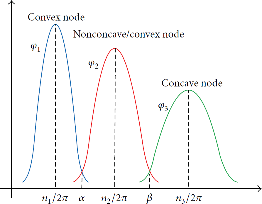
Distribution curve when k is 2.

The normal probability density function is

$$\begin{array}{cc}& f\left(x\right)=\frac{\mathrm{1}}{\sqrt{\mathrm{2}\pi }\sigma }\exp \left(-\frac{{\left(x-\mu \right)}^{\mathrm{2}}}{\mathrm{2}{\sigma }^{\mathrm{2}}}\right),\end{array}$$

(17)

where ${\mu }_{\mathrm{1}}=n_{\mathrm{1}}/\mathrm{2}\pi$ , ${\sigma }_{\mathrm{1}}^{\mathrm{2}}=n_{\mathrm{1}}/\mathrm{108}{\pi }^{\mathrm{2}}$ , ${\mu }_{\mathrm{2}}=n_{\mathrm{2}}/\mathrm{2}\pi$ , and ${\sigma }_{\mathrm{2}}^{\mathrm{2}}=n_{\mathrm{2}}/\mathrm{108}{\pi }^{\mathrm{2}}$ . Then,

$$\begin{array}{cc}& \frac{\mathrm{1}}{\sqrt{\mathrm{2}\pi }{\sigma }_{\mathrm{1}}}\exp \left(-\frac{{\left(\alpha -{\mu }_{\mathrm{1}}\right)}^{\mathrm{2}}}{\mathrm{2}{\sigma }_{\mathrm{1}}^{\mathrm{2}}}\right)=\frac{\mathrm{1}}{\sqrt{\mathrm{2}\pi }{\sigma }_{\mathrm{2}}}\exp \left(-\frac{{\left(\alpha -{\mu }_{\mathrm{2}}\right)}^{\mathrm{2}}}{\mathrm{2}{\sigma }_{\mathrm{2}}^{\mathrm{2}}}\right).\end{array}$$

(18)

Thus,

$$\begin{array}{cc}& \alpha \approx \mathrm{0.729}.\end{array}$$

(19)

The corresponding minimum hop count of α is $n_{\mathrm{1}}^{\ast }=\alpha ·\mathrm{2}\pi \approx \mathrm{4.6}$ . The value of β can be calculated in the same way. Thus, $\beta \approx \mathrm{1.332}$ , and its corresponding minimum hop count is $n_{\mathrm{2}}^{\ast }=\beta ·\mathrm{2}\pi \approx \mathrm{8.4}$ . Since the hop count value is a positive integer, it is easy to know that, in the case of $k=\mathrm{2}$ , when the minimum hop count $n\le \mathrm{4}$ , $P_i$ is identified as a convex node, when $\mathrm{5}\le n\le \mathrm{8}$ , $P_i$ is a nonconcave/convex node, and when $n\ge \mathrm{9}$ , $P_i$ is a concave node.

Let k, respectively, be 3, 4, and 5, and calculate the corresponding values of α and β. Then, the corrected value of the minimum hop count n is determined and the concavity or convexity of $P_i$ can be identified, as is shown in Table 2.

Table 2

Final concave/convex node recognition criterion in different values of k.

k	Convex node	Nonconcave/convex node	Concave node
2	$$n\le 4$$	$$5\le n\le 8$$	$$n\ge 9$$
3	$$n\le 7$$	$$8\le n\le \mathrm{13}$$	$$n\ge \mathrm{14}$$
4	$$n\le 9$$	$$\mathrm{10}\le n\le \mathrm{18}$$	$$n\ge \mathrm{19}$$
5	$$n\le \mathrm{12}$$	$$\mathrm{13}\le n\le \mathrm{23}$$	$$n\ge \mathrm{24}$$

Assume that there are M boundary nodes in the network, represented by $P_i$ , $i=\mathrm{1,2},\dots ,M$ . For an arbitrary node $P_i\in \omega$ , it can use its k-hop neighboring boundary nodes $p_{i\mathrm{1}}$ and $p_{i\mathrm{2}}$ to identify the concavity or convexity of itself, where $k\in \{\mathrm{2,3},\mathrm{4,5}\}$ . According to the above-mentioned mathematical analysis and criterion, we give the concave/convex node recognition algorithm based on the minimum hop count as follows, which includes four steps.

Step 1.

For each boundary node $P_i$ , $P_i$ obtains its k-hop neighboring boundary nodes $p_{i\mathrm{1}}$ and $p_{i\mathrm{2}}$ ; that is, $p_{i\mathrm{1}},p_{i\mathrm{2}}\in \omega$ and $p_{i\mathrm{1}},p_{i\mathrm{2}}\in \partial N_{\mathrm{2}}(P_i)$ , where $k\in \{\mathrm{2,3},\mathrm{4,5}\}$ , and its value is preset by the system.

Step 2.

If there are $p_{i\mathrm{1}}$ and $p_{i\mathrm{2}}$ that meet the condition in Step 1, then turn to Step 3. Otherwise, $P_i$ gives up the concavity/convexity identification of itself.

Step 3.

$P_i$ derives the minimum hop count n between $p_{i\mathrm{1}}$ and $p_{i\mathrm{2}}$ .

Step 4.

$P_i$ identifies its concavity or convexity by using the criterion in Table 2.

4.2.3. Concave/Convex Node Cleansing

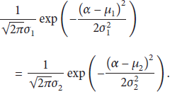
After concave/convex node recognition algorithm, the concavity or convexity of each boundary node has been identified. Since the sensor network is discrete, it is possible that a nonconcave node which is in the nonconcave region is identified as a concave node by mistake. These mistaken concave nodes often appear in an isolate way. In contrast, there always are several concave nodes in a concave area; that is, real concave nodes always gather together (seen in Figures 8(c), 9(c), and 10(c), e.g.; the black nodes are ordinary nodes, and the red nodes are boundary nodes. The nodes with peach circles are concave nodes, and those with cyan circles are convex nodes. Other red nodes without any circles are nonconcave/convex nodes). Therefore, the isolate concave node can be directly eliminated from the recognition result (to simplify our algorithm, we define isolate concave node as the concave node which has no concave node within its two hops; similarly, isolate convex node is the convex node which has no convex node within its two hops), as well as the isolate convex node.

Figure 8

Region decomposition of L-shape network. 763 nodes are uniformly distributed, and average degree of the network is 9.13. (a) Original map. (b) Boundary recognition result. The red nodes are boundary nodes. (c) Concave/convex node recognition result, $k=\mathrm{3}$ . The nodes with peach circles are concave nodes, and nodes with cyan circles are convex nodes. (d) Optimal concave/convex nodes. Optimal concave nodes are marked with peach, and optimal convex nodes are marked with cyan. (e) Boundary segmentation result. Different color and markers represent different boundary branches. (f) Region decomposition result. The same color nodes belong to one subregion.

Figure 9

Region decomposition of C-shape network. 1295 nodes are uniformly distributed, and average degree of the network is 9.04. (a) Original map. (b) Boundary recognition result. The red nodes are boundary nodes. (c) Concave/convex node recognition result, $k=\mathrm{3}$ . The nodes with peach circles are concave nodes, and the nodes with cyan circles are convex nodes. (d) Optimal concave/convex nodes. Optimal concave nodes are marked with peach, and optimal convex nodes are marked with cyan. (e) Boundary segmentation result. Different color and markers represent different boundary branches. (f) Region decomposition result. The same color nodes belong to one subregion.

Figure 10

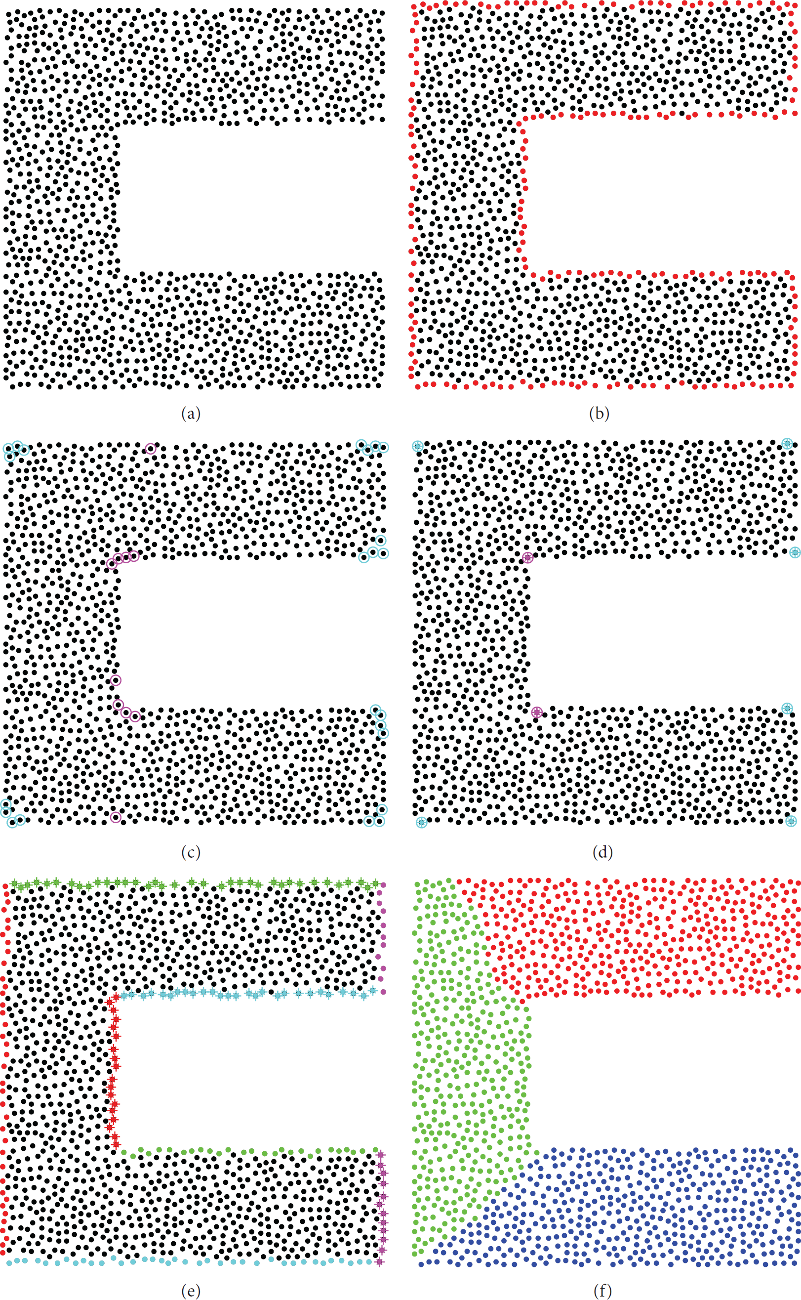
Region decomposition of single-window-shape network. 1505 nodes are uniformly distributed, and average degree of the network is 9.01. (a) Original map. (b) Boundary recognition result. The red nodes are boundary nodes. (c) Concave/convex node recognition result, $k=\mathrm{3}$ . The nodes with peach circles are concave nodes, and the nodes with cyan circles are convex nodes. (d) Optimal concave/convex nodes. Optimal concave nodes are marked with peach, and optimal convex nodes are marked with cyan. (e) Boundary segmentation result. Different color and markers represent different boundary branches. (f) Region decomposition result. The same color nodes belong to one subregion.

For the concave nodes that gather together in one concave area, since larger concavity of the concave node will lead to larger deviation between hop count distance and the Euclidean distance, we choose the concave node with the maximum concavity as the optimal concave node in this area. In our algorithm, the node with maximum concavity corresponds to the node which is with the biggest minimum hop count between its two k-hop neighboring boundary nodes. It is possible that in some concave area there may be more than one concave node with the same biggest minimum hop count. For this case, we randomly choose one of them as the optimal concave node. The above process is called cleansing process.

Similarly, we use the cleansing criterion to cleanse the convex node in the network. The difference is that the convex node with the smallest minimum hop count should be taken as the optimal convex node. If there is more than one convex nodes with the same smallest minimum hop count in a convex area, we randomly choose one of them as the optimal convex node.

Through the cleansing criterion, the optimal concave/convex node is obtained. For example, the cleansing results of Figures 8(c), 9(c), and 10(c), respectively, are Figures 8(d), 9(d), and 10(d), where the optimal concave nodes are marked with peach and the optimal convex nodes are marked with cyan.

4.3. Boundary Segmentation

Assume that the boundary of the network is fully connected. For simplicity, the optimal concave and convex nodes are called the optimal nodes in this section. In order to segment the boundary, we use the optimal nodes to flood Boundary Segmentation PacKeT (BS-PKT) among the boundary nodes. Each BS-PKT concludes the ID number of the node which generates the BS-PKT. When a boundary node A receives a BS-PKT, A deals the current BS-PKT with the following ways:

• (1)

If A is not a boundary node, A discards BS-PKT.

(2)

If A is a boundary node but not an optimal node, A records the ID number in BS-PKT and sends BD-PKT to its neighbor nodes.

(3)

If A is both a boundary node and an optimal node, but A has not recorded any ID number of other optimal nodes, then A records the ID number in BS-PKT and does not send BS-PKT anymore.

(4)

If A is both a boundary node and an optimal node, and A has recorded an ID number of another optimal node, A discards the BS-PKT.

After flooding, each boundary node will record two different ID numbers of the optimal nodes. Assume the ID numbers, respectively, are I and J. Let ${\mathrm{B}\mathrm{o}\mathrm{u}\mathrm{n}\mathrm{d}}_{\mathrm{I}\mathrm{D}}=[I,J]$ . Only when two boundary nodes have the same I and J is their ${\mathrm{B}\mathrm{o}\mathrm{u}\mathrm{n}\mathrm{d}}_{\mathrm{I}\mathrm{D}}$ defined to be equal. In such situation, the boundary nodes which have the same ${\mathrm{B}\mathrm{o}\mathrm{u}\mathrm{n}\mathrm{d}}_{\mathrm{I}\mathrm{D}}$ belong to the same boundary branch, and ${\mathrm{B}\mathrm{o}\mathrm{u}\mathrm{n}\mathrm{d}}_{\mathrm{I}\mathrm{D}}$ is the boundary number of this branch. Thus, the boundary of the network is segmented (e.g., Figures 8(e), 9(e), and 10(e) are the boundary segmentation results of the networks, where different color and markers represent different boundary branches).

4.4. Region Decomposition

For a fully connected anisotropic network, define U as the set of the optimal concave nodes. For an arbitrary optimal concave node $q_i\in U$ , its two k-hop neighboring boundary nodes have been obtained in the concave/convex node recognition process. For simplicity, the k-hop neighboring boundary nodes are also called neighboring boundary nodes.

To decompose the network, all neighboring boundary nodes of the optimal concave nodes flood Region Decomposition PacKeT (RD-PKT) in the network. Each RD-PKT concludes the ID number of the node which generates this RD-PKT and the boundary number ${\mathrm{B}\mathrm{o}\mathrm{u}\mathrm{n}\mathrm{d}}_{\mathrm{I}\mathrm{D}}$ recorded by the node. The format of RD-PKT is (ID, ${\mathrm{B}\mathrm{o}\mathrm{u}\mathrm{n}\mathrm{d}}_{\mathrm{I}\mathrm{D}}$ ). When an arbitrary node B receives a RD-PKT for the first time, B records (ID, ${\mathrm{B}\mathrm{o}\mathrm{u}\mathrm{n}\mathrm{d}}_{\mathrm{I}\mathrm{D}}$ ) in RD-PKT and sends RD-PKT to its neighbor nodes; if B receives a RD-PKT not for the first time, B discards it directly. This policy ensures that most nodes will receive only one RD-PKT from the closest neighboring boundary node.

By this means, each node in the network will record only one RD-PKT, in which the ID and ${\mathrm{B}\mathrm{o}\mathrm{u}\mathrm{n}\mathrm{d}}_{\mathrm{I}\mathrm{D}}$ number of the corresponding neighboring boundary node are included. The nodes which have the same ID number belong to one subregion; then, the original region decomposition result is obtained. To avoid the network from decomposing to too many subregions, the nodes with the same ${\mathrm{B}\mathrm{o}\mathrm{u}\mathrm{n}\mathrm{d}}_{\mathrm{I}\mathrm{D}}$ can be merged to one subregion. Finally, an anisotropic network is decomposed into many different subnetworks. See Figures 8(f), 9(f), and 10(f), for example; different colors represent different subnetworks. It is obvious that there is no longer serious bent path between far-away nodes in each subnetwork. Thus, each subnetwork can be considered as an isotropic network.

In summary, after boundary recognition, concave/convex node recognition and cleansing, boundary segmentation, and region decomposition, an anisotropic network finally is decomposed into several different isotropic subnetworks. During the process of HCD, we only need to use the connectivity information of the network, without any additional hardware on sensor nodes. As a range-free localization algorithm, the complexity of communication cost of DV-Hop is $O(N·m)$ . Here, N and m are the numbers of sensor nodes and anchor nodes, respectively. For HCD (Hop Count Based Decomposition) scheme, the complexity of communication cost is $O(N)$ . Since our proposed HCD-DV-Hop scheme is composed of HCD and DV-Hop, the complexity of communication cost of HCD-DV-Hop is the same as DV-Hop.

5. Performance Evaluation

To evaluate the proposed algorithm, we simulate on three typical anisotropic network topologies: L-shape, C-shape, and single-window-shape network topologies. In simulations, nodes are uniformly distributed. All nodes have the same communication range. Two nodes are connected if and only if the Euclidean distance between them is smaller than a given communication radius R.

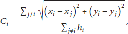
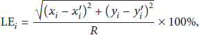
We compare our algorithm with DV-Hop. For comparison, two metrics are used in this section: LE (localization error) and ALE (average localization error). The LE of an unknown node i is calculated by

$$\begin{array}{cc}& {\text{LE}}_i=\frac{\sqrt{{\left(x_i-x_i^{\prime }\right)}^{\mathrm{2}}+{\left(y_i-y_i^{\prime }\right)}^{\mathrm{2}}}}{R}\times \mathrm{100}\%,\end{array}$$

(20)

where $(x_i,y_i)$ is the real location of node i and $(x_i^{\prime },y_i^{\prime })$ is the estimated location which is obtained by the localization algorithm. ALE is the average localization error of all unknown nodes in the network, it can be computed by

$$\begin{array}{cc}& \text{ALE}=\frac{\mathrm{1}}{N}{\displaystyle \sum }_{i=\mathrm{1}}^N{\text{LE}}_i,\end{array}$$

(21)

where N is the number of unknown nodes. It is obvious that the smaller the LE and ALE, the better the localization algorithm.

5.1. Region Decomposition

Given three typical anisotropic networks, L-shape network, C-shape network, and single-window-shape network, as shown in Figures 8(a), 9(a), and 10(a), respectively, nodes are uniformly distributed in each network. The communication radius is 40 m. First we use HCD (Hop Count Based Decomposition algorithm) to decompose the networks. Simulation results are shown in Figures 8–10.

5.2. Performance Evaluation of Algorithms under Certain Communication Radius and Ratio of Anchor Node

Here the communication radius is 40 m and the ratio of anchor node is 10%. Anchors are randomly distributed in the networks.

For each anisotropic network, after decomposing, DV-Hop is carried out in each subnetwork. Thus, the LE (localization error) of each unknown node is obtained through HCD-DV-Hop algorithm, as shown in Figures 11(a), 11(c), and 11(e). The LE obtained by DV-Hop is shown in Figures 11(b), 11(d), and 11(f), respectively. Table 3 gives the corresponding ALE (average localization error) of each network by HCD-DV-Hop and DV-Hop.

Table 3

ALE of each network by HCD-DV-Hop and DV-Hop algorithm.

Network topology	HCD-DV-Hop	DV-Hop
L-shape	57.8%	172.4%
C-shape	65.8%	595.3%
Single-window-shape	65.7%	161.3%

Figure 11

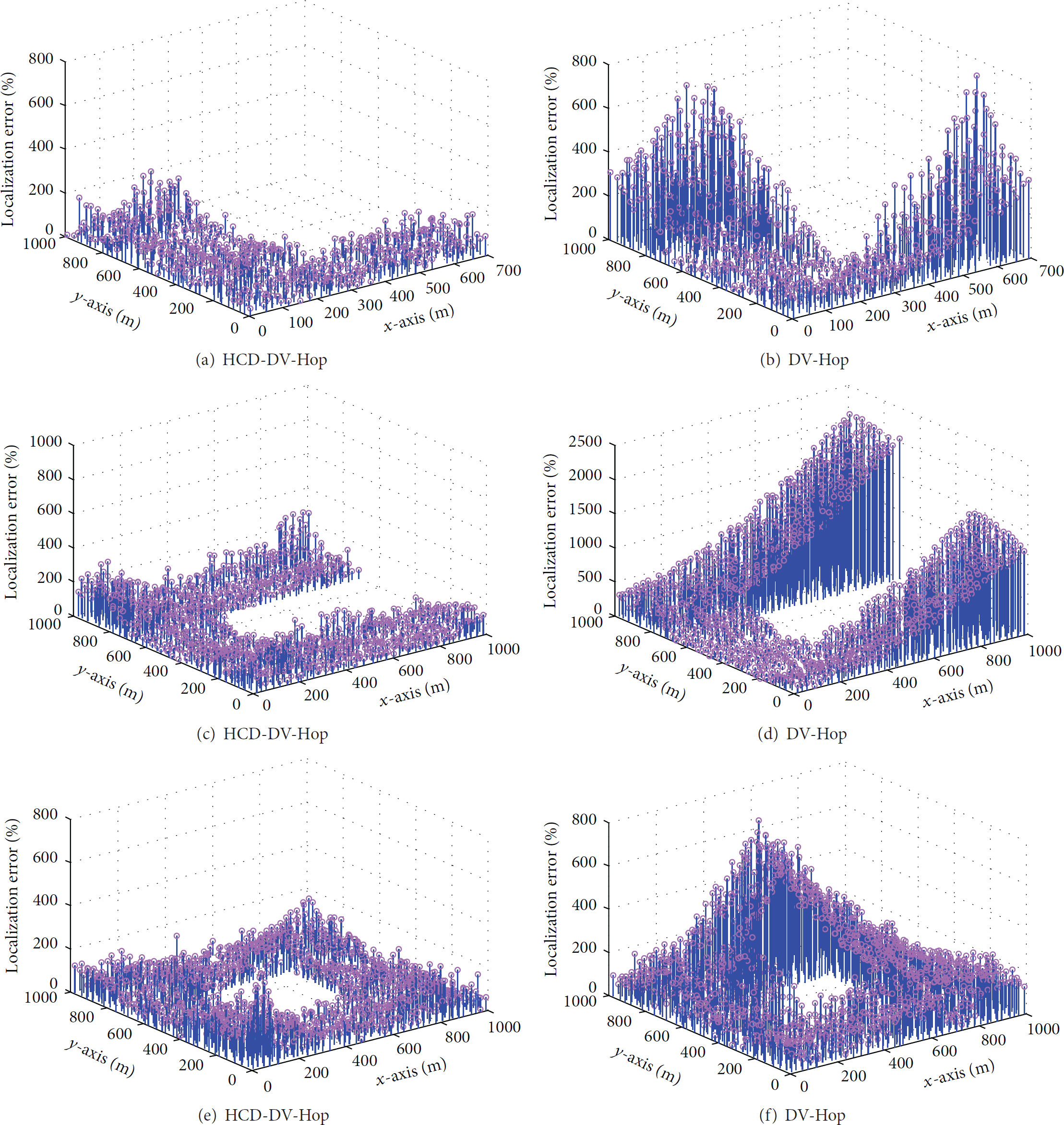
LE (localization error) of each network by different algorithms. (a) LE of L-shape network by HCD-DV-Hop. (b) LE of L-shape network by DV-Hop. (c) LE of C-shape network by HCD-DV-Hop. (d) LE of C-shape network by DV-Hop. (e) LE of single-window-shape network by HCD-DV-Hop. (f) LE of single-window-shape network by DV-Hop.

As shown in Figure 11 and Table 3, we found that whatever the network topology is, HCD-DV-Hop can effectively reduce the LE of most unknown nodes compared with DV-Hop, and the ALE obtained by HCD-DV-Hop is much smaller than that by DV-Hop. Obviously, the reason is that HCD-DV-Hop uses decomposition scheme to avoid serious bent path between far-away nodes participating in localization.

5.3. Performance Evaluation of Algorithms under Different Ratios of Anchor Node

Given a certain communication radius (take 40 m as the communication radius in the simulations), we examine the performance of HCD-DV-Hop and DV-Hop under different ratios of anchor node. In simulations, we randomly generated 200 networks and computed the ALE of each network. Finally, we take the average value of the 200 ALE as the average error under each ratio of anchor node. Simulation results of L-shape, C-shape, and single-window-shape network are shown in Figures 12(a), 12(b), and 12(c), respectively.

Figure 12

Average error under different ratios of anchor node.

Figure 12 shows that, for different communication radius in Lshape, C-shape, and Single-window-shape networks, compared with DV-Hop, the average error of HCD-DV-Hop is significantly decreased. That is, HCD-DV-Hop performs much better in localization than DV-Hop.

5.4. Performance Evaluation of Algorithms under Different Communication Radius

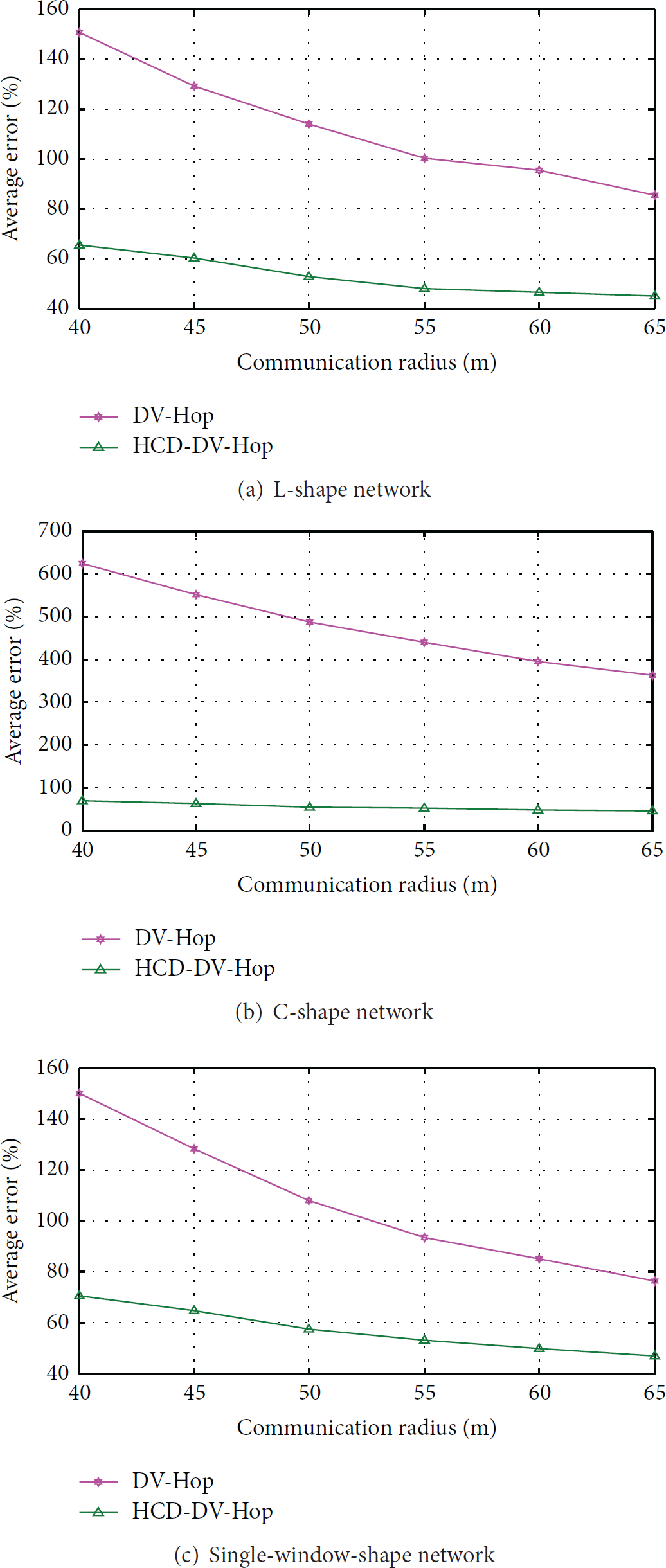
Given a certain ratio of anchor node (take 10% as the ratio of anchor node in the simulations), we examine the performance of HCD-DV-Hop and DV-Hop under different communication radius. In simulations, we randomly generated 200 networks and computed the ALE of each network. Finally, we take the average value of the 200 ALE as the average error under each communication radius. Simulation results of L-shape, C-shape, and single-window-shape network are shown in Figures 13(a), 13(b), and 13(c), respectively.

Figure 13

Average error under different communication radius.

From Figure 13, we observe that the average error of our proposed HCD-DV-Hop is much smaller than that of DV-Hop, which obviously proves the localization advantage of HCD-DV-Hop in anisotropic networks.

6. Conclusion and Future Work

In this paper, we have proposed a novel decomposition based localization (HCD-DV-Hop) scheme for anisotropic sensor networks. The main idea of HCD-DV-Hop is first decomposing an anisotropic network into several different isotropic subnetworks in order to avoid the influence of holes or obstacles on the shortest communication path between far-away nodes; then, the typical range-free DV-Hop algorithm is used for node localization in each subnetwork. The HCD algorithm is the core of HCD-DV-Hop. It includes boundary recognition, concave/convex node recognition and cleansing, boundary segmentation, and region decomposition. All of these steps are distributed and only require network connectivity information. Simulation results show that no matter how node communication radius or the ratio of anchor node changes, compared with DV-Hop algorithm, the proposed HCD-DV-Hop scheme can effectively reduce localization error in anisotropic networks without increasing the complexity of the algorithm.

In HCD-DV-Hop, we use the typical range-free DV-Hop algorithm to achieve node localization in each isotropic subnetwork. As HCD scheme is able to decompose an anisotropic network into different isotropic subnetworks, it can be used to investigate the localization performance on the combination of HCD with other range-free algorithms. Additionally, the proposed HCD-DV-Hop scheme is designed for 2D networks. In our future research, we will explore the possible improvements on HCD-DV-Hop in order to adapt to 3D networks.