Living Space Evolution: A New Crowd Based Computational Approach

Abstract

Inspired by the life cycle and survival of the fittest and combined with the consideration of living space information, a new computational intelligence approach, namely, living space evolution (LSE), is presented. LSE has reflected two new ideas. One is living space evolution: under the guidance of living space information, the offspring of life concentrate and evolve continuously towards richer living spaces. The other is multiple offspring reproduction: simulating real life in nature, a life can reproduce multiple offspring within one generation. In this work, LSE dynamic model, its flow, and pseudocodes are described in detail. A digital simulation has shown the procedure of LSE living space evolution. Furthermore, two applications of using LSE are employed to demonstrate its effectiveness and applicability. One is to apply it to the optimization for continuous functions, and the other is to use it as an optimization tool for routing protocol in wireless sensor network that is a discrete problem in real world. Research has shown that LSE is effective for the optimization for the continuous functions and also applicable for the discrete problem in real world. In addition, LSE has a special ability to balance search process from exploration to exploitation gradually.

1. Introduction

Bioinspired computation [1, 2] opens up a new way for computational intelligence [3–5]. The basic idea of bioinspired computation is to seek inspiration and methods of problem solving from the natural biological systems. Under the guidance of bioinspired ideas, a series of approaches of computational intelligence have been created successively, including artificial neural networks, evolutionary computation, swarm intelligence techniques, and artificial immune systems. These approaches imitate biological neural structure and various behaviors, numerous applications of which [6–9] have proved their effectiveness and reliability.

Bioinspired computation is an active area of computer science [1] and tries to simulate some characteristics of biological systems in nature from the following aspects.

(1) Mimic Biological Neural Structure: Artificial Neural Network. Artificial neural network (ANN), firstly reported by Warren McCulloch and Walter Pitts with the idea of mathematically simulating biological neural structures, is multi-input and multioutput computing system made up of a number of simple and highly interconnected processing elements known as neurons, which processes information by its dynamic state response to external inputs. The advantage of ANN is that complex nonlinear relationships can be easily handled even when the exact nature of such behavior is not well defined [10].

(2) Mimic the Process of Biological Evolution: Evolutionary Computation. Evolutionary computation (EC) is produced based on principles of biological evolution, such as natural selection and genetic inheritance [11, 12]. While efficient utilization of computational resources is increasing, EC is making rapid progress, and its social recognition and need as applied technology are increasing [13–16]. Today, there are a variety of algorithms involved in EC. Among them, the four well-known EC variants are evolutionary programming (EP), evolution strategy (ES), genetic algorithm (GA), and genetic programming (GP).

In addition, a new evolutionary algorithm (EA), namely, Backtracking Search Optimization Algorithm (BSA), is very recently developed by Civicioglu in 2013 [17]. Unlike many search algorithms, BSA has a single control parameter and a simple structure. BSA's strategies for generating trial populations and controlling the amplitude of the search-direction matrix and search-space boundaries give it very powerful exploration and exploitation capabilities. BSA seems to be very promising [18].

(3) Mimic Biological Swarm Behaviors: Swarm Intelligence. Swarm intelligence [19, 20], inspired by the behaviors of some social living beings such as bird flocks and fish schools and colonies of ants, termites, bees, and wasps, is a discipline that deals with natural and artificial systems composed of many individuals that coordinate their activities using decentralized control and self-organization [21]. The most well-known swarm intelligence techniques include particle swarm optimization (PSO) [22, 23], ant colony optimization (ACO) [24, 25], and artificial bee colony algorithm (ABC) [26].

(4) Mimic Biological Immune System: Artificial Immune System. Artificial immune system (AIS), inspired by the biological immune system, is an emerging kind of computational paradigms that belong to the computational intelligence family. The work in the field of AIS was initiated by Farmer [27]. In their research, a dynamic model of the immune system that was simple enough to be simulated on a computer where the antibody-antibody and antibody-antigen reactions are simulated via complementary matching strings was introduced [28].

As introduced above, the primary approaches of bioinspired computation are inspired from some the characteristics of the biological systems in nature such as different biological behaviors or structures, but they have a common drawback in that they usually neglect the biological living condition. Throughout the life phenomena in nature, life cycle and survival of the fittest as timeless, constant, and universal natural laws are two basic survival rules for life's individual and colony. Following these rules, lives living on the earth reproduce offspring from generation to generation and are born again and again for hundreds of millions of years. However, by careful analysis, we know that lives cannot live without a certain biological living condition. Therefore, biological living condition is an essential factor for life's living and evolution. Here, biological living condition is referred to as living space information. In this paper, computer and program are employed to simulate the principles of life cycle and survival of the fittest, combined with the consideration of living space information, so as to establish a new crowd based computational intelligence approach, namely, living space evolution (LSE). LSE has reflected two new ideas. One is living space evolution: under the guidance of living space information, the offspring of life concentrate and evolve continuously towards richer living spaces. The other is multiple offspring reproduction: a life can reproduce multiple offspring within one generation, which stimulates real lives in nature.

The rest of the paper is organized as follows. LSE dynamic model is set up in Section 2. Section 3 gives the description of LSE algorithm in detail. Digital demonstration in Section 4 illustrates the procedure of LSE. Examples for LSE's application are presented in Section 5. Finally, conclusions are drawn in Section 6.

2. LSE Dynamic Model

Life is cyclic, which is a natural law. Life cycle has two meanings. The first is that the lifetime of a life is limited. The second is that the life has the ability to reproduce offspring under certain conditions. On the other hand, life must obey the rule of survival of the fittest which is another natural law in order to continue to be alive on the earth. Subject to these two laws, the life's significance is that it looks for richer places on the earth and captures adequate nutrition then survives and reproduces. Here richer places mean the places where life has better biological living condition. Here, biological living condition is referred to as living space information.

In nature, each life's lifetime is different, and its process of reproducing offspring is different too. For the ease of simulation, a simplified dynamic model is extracted from the two principles of life cycle and survival of the fittest and from the combination with the consideration of life's living space information, which is named as living space evolution (LSE), as shown in Algorithm 1.

Algorithm 1: LSE dynamic model.

Step  1. Initialization

   Set initial swarm of life.

   Set initial living space.

Step  2. Divide the initial living space to each life in the initial swarm of life, namely, assign living space for each life.

Step  3. Each life gets nutrient in its living space.

Step  4. For each life, do:

{

Step  4.1. Acquires nutrition in its living space.

Step  4.2. The life that capture adequate nutrition survives, otherwise dies.

Step  4.3. The surviving life reproduces its multiple offspring in its living spaces.

Step  4.4. The offspring inherit and share their parental life's living spaces, namely, assign living subspace for each offspring.

Step  4.5. The parental life die after reproduction.

Step  4.6. Each offspring gets nutrient in its living subspace.

}

Step  5. For each offspring, do:

{

Step  5.1. The offspring that capture adequate nutrition survives, otherwise dies.

Step  5.2. The surviving offspring reproduces its multiple new offspring in its living subspaces.

Step  5.3. The new offspring inherit and share their parental offspring's living subspaces, namely, assign living subspace for each

new offspring.

Step  5.4. The parental offspring die after reproduction.

Step  5.5. Each new offspring gets nutrient in its living subspace.

}

Step  6. Go to Step  5

From Algorithm 1, we can see that there are five assumptions in the LSE dynamic model.

• (1)

A life acquires nutrition in its living space or subspace.

(2)

A life that captures adequate nutrition survives; otherwise, it dies.

(3)

One surviving life can reproduce multiple offspring at the same time. After reproducing one generation of offspring, the parental life dies immediately.

(4)

The offspring inherit and share their parental living subspaces only.

(5)

All lives reproduce offspring in a synchronous manner.

From the LSE dynamic model, we can know that its running process can be described as follows: life reproduces its multiple offspring from generation to generation, but only the offspring that capture adequate nutrition in their living spaces can survive; other offspring with their living spaces are eliminated. By this way, life’ living spaces continually evolve. In other words, in order to survive, the offspring of life concentrate and evolve continuously towards the richer living spaces for ever and never stopped.

3. Description of LSE Algorithm

3.1. Basic Concepts

First of all, the following concepts should be defined in order to describe LSE algorithm.

Definition 1 (life).

Life is an abstract entity. Living space and living condition, here, namely, nutrition, are the two basic surviving elements that life depends on. Life's spatial coordinates are defined at the midpoint in its living space.

Definition 2 (living space).

Living space denotes the spatial range where a life is located in. Life monopolizes its living space. When life reproduces offspring, its offspring inherit and share its living space.

Definition 3 (nutrition).

Nutrition represents the resource that life depends on. Here, the size of nutrition is supposed to be a fixed distribution in living space.

Definition 4 (threshold nutrition).

Threshold nutrition is defined as a basic amount of nutrition; a life that acquires nutrition bigger than or equal to threshold nutrition survives; otherwise, it dies.

Definition 5 (richer living space).

Richer living space stands for the living space with richer nutrition. There are two cases: for maximum optimizations, richer living space means the living space with bigger fitness, whereas, for minimum optimizations, it means the living space with smaller fitness.

3.2. Basic Assumptions

To create LSE algorithm, the following assumptions should be introduced too.

Assumption 1 (reproduction).

When the acquired nutrition is bigger than or equal to the threshold nutrition, life can reproduce offspring, whereas if the acquired nutrition is smaller than the threshold nutrition, life cannot reproduce offspring.

Assumption 2 (asexual reproduction).

Life reproduces offspring by asexual means.

Assumption 3 (multiple offspring reproduction).

One life can reproduce multiple offspring within one generation.

Assumption 4 (inheritance and share).

Offspring inherit and share their parental life's living space. But the living space where life cannot reproduce offspring will be naturally discarded because no offspring can inherit and share the living space.

Assumption 5 (survival of the fittest).

When acquiring nutrition bigger than or equal to the threshold nutrition, life survives and reproduces offspring; otherwise, life dies immediately.

Assumption 6 (life cycle).

There are two cases for life's termination. Life dies immediately while acquiring nutrition smaller than threshold nutrition or dies immediately after reproducing one generation's offspring.

Assumption 7 (nutrition calculation).

The size of nutrition in living space is supposed to be a fixed distribution and calculated by means of its distribution function marked as $f()$ with coordinates at midpoint in the living space.

3.3. Flow of LSE Algorithm

Based on the concepts defined and the assumptions introduced above and according to the LSE dynamic model in Algorithm 1, we can get the flow of LSE algorithm that is described in Algorithm 2.

Algorithm 2: Flow of LSE algorithm.

Step  1. Initialization.

   Set the number of lives in initial swarm of life;

   Set the scope of initial living space;

   Set the number of offspring reproduced by each surviving life;

   Set nutrition distribution function $f()$ .

   Set the maximum number of reproduction generations;

Step  2. Divide uniformly the initial living space to each life in the initial swarm of life, namely, assign uniformly living space for

each life.

Step  3. Each life acquires nutrition in its living space, which is calculated by nutrition distribution function $f()$ with coordinates

at midpoint of its living space.

Step  4. For each life, do:

{

Step  4.1. Calculate threshold nutrition that is equal to the average of nutrition acquired by all lives at present.

Step  4.2. The lives that acquire nutrition bigger than or equal to threshold nutrition survive, otherwise die.

Step  4.3. The surviving lives reproduce multiple offspring in their living spaces.

Step  4.4. The offspring inherit and share uniformly their parental life's living spaces, namely, assign uniformly living subspace

for each offspring.

Step  4.5. The parental life dies after reproduction.

Step  4.6. Each offspring acquires nutrition in its living subspace, which is calculated by nutrition distribution function $f()$ with

coordinates at midpoint of its living subspace.

}

Step  5. Judge whether the maximum number of reproduction generations is reached. If reached, go to Step  8.

Step  6. For each offspring, do:

{

Step  6.1. Calculate threshold nutrition that is equal to the average of nutrition acquired by all offspring at present.

Step  6.2. The offspring that acquire nutrition bigger than or equal to threshold nutrition survive, otherwise die.

Step  6.3. The surviving offspring reproduce its mutiple new offspring in its living subspaces.

Step  6.4. The new offspring inherit and share uniformy their parental offspring's living subspaces,

namely, assign uniformly living subspace for each new offspring.

Step  6.5. The parental offspring die after reproduction.

Step  6.6. Each new offspring acquires nutrition in its living subspace, which is calculated by nutrition distribution function $f()$

with coordinates at midpoint of its living subspace.

}

Step  7. Go to Step  5

Step  8. The end

In Algorithm 2, Step 1 finishes initialization for LSE algorithm, including setting the number of lives in initial swarm of life, the ranges of initial living spaces, the number of offspring reproduced by each surviving life, and the maximum number of reproduction generations and giving the nutrition distribution function $f()$ . Step 2 assigns uniformly living space for each life. In Step 3, each life acquires nutrition in its living space, calculated by nutrition distribution function $f()$ with coordinates at midpoint of its living space.

Step 4 enters a loop for each life, in which Step $4.1$ calculates threshold nutrition that is equal to the average of nutrition acquired by all lives at present. In Step 4.2, the lives that acquire nutrition bigger than or equal to the threshold nutrition survive; otherwise, they die. In Step 4.3, the surviving lives reproduce its multiple offspring in their living spaces. In Step 4.4, the offspring inherit and share uniformly their parental life's living spaces; namely, they assign uniformly living subspace for each offspring. In Step 4.5, the parental life dies after reproduction. In Step 4.6, each offspring acquires nutrition in its living subspace, which is calculated by nutrition distribution function $f()$ with coordinates at midpoint of its living subspace.

Step 5 judges whether the maximum number of reproduction generations is reached. If it is reached, go to Step 8 that ends the LSE algorithm.

Step 6 enters a loop for each offspring, in which its procedures and operations are same as Step 4. Step 7 goes to Step 5. Step 8 is the end of the LSE algorithm.

We need to pay special attention to the fact that Steps 4 and 6 accomplish living space evolution and multiple offspring reproduction, respectively. On the one hand, within the course of living space evolution, a portion of lives with their living spaces are eliminated. On the other hand, multiple offspring reproduction can continuously supplement fresh lives in order to maintain a certain number of ones. Therefore, multiple offspring reproduction is the prerequisite and guarantee for achieving living space evolution.

3.4. Implementation of LSE Algorithm

Pseudocodes of LSE algorithm are summarized as shown in Pseudocode 1.

Pseudocode 1: Pseudocodes of LSE algorithm.

Step  1. Initialization

Set initial n-dimensional living space as $U=\left\{x_i\hspace{0.17em}|\hspace{0.17em}{a}_i\le x_i\le b_i\right\}$ , $i=\mathrm{1},\dots ,n$ , $n\in N^{+}$

Set the number of lives in initial swarm equal to $N^n$ , $N\in N^{+}$ , n is the number of dimensions of living space.

Set the number of offspring reproduced by each surviving life equal to ${N_{\mathrm{n}\mathrm{e}\mathrm{x}\mathrm{t}}}^n$ , $N_{\mathrm{n}\mathrm{e}\mathrm{x}\mathrm{t}}\in N^{+}$ , n is the number of dimensions of living

space.

Set the nutrition distribution function in living space equal to $f(x_{\mathrm{1}},x_{\mathrm{2}},\dots ,x_n)$ , $a_i\le x_i\le b_i$ , $i=\mathrm{1},\dots ,n$ , $n\in N^{+}$

Set the adjustment coefficient $c=\mathrm{1}$

Set the initial value of present reproduction generation $t=\mathrm{1}$

Set the maximum number of reproduction generations equal to T

Step  2. Share living space

Set the coordinates of lives in ith dimensional living space marked as $p_{ij}$ .

$p_{ij}=(x_i\hspace{0.17em}|\hspace{0.17em}{a}_i\le x_i\le b_i)$ , $i=\mathrm{1},\dots ,n$ , $j=\mathrm{1},\dots ,N$

Set the interval of sharing evenly ith dimensional living space marked as ${\mathrm{\sigma }}_i$ .

${\mathrm{\sigma }}_i=\left(b_i-a_i\right)/N$ / ${}^{\mathit{\ast }}$ Interval of sharing uniformly ith dimensional living space ${}^{\mathit{\ast }}$ /

Set $p_{ij}=a_i+(\mathrm{1}/\mathrm{2}){\mathrm{\sigma }}_i\hspace{0.17em}|\hspace{0.17em}j=\mathrm{1}$ and $p_{i(j+\mathrm{1})}=p_{ij}+{\mathrm{\sigma }}_i\hspace{0.17em}|\hspace{0.17em}j\ge \mathrm{1}$ / ${}^{\mathit{\ast }}$ Relationship of coordinates of lives in ith dimensional living space.

The coordinate range of each life in ith dimensional living subspace is [ $p_{ij}-\left(\mathrm{1}/\mathrm{2}\right){\mathrm{\sigma }}_i$ , $p_{ij}+\left(\mathrm{1}/\mathrm{2}\right){\mathrm{\sigma }}_i$ ], and its length is ${\mathrm{\sigma }}_i$    ${}^{\mathit{\ast }}$ /

Where $i=\mathrm{1},\dots ,n$ , $j=\mathrm{1,2},\dots ,N$

Step  3. Acquire nutrition

Calculate $f(x_{\mathrm{1}},x_{\mathrm{2}},\dots ,x_n)$ for all lives with coordinates at midpoints in their living subspaces.

Step  4. Calculate threshold nutrition

Set threshold nutrition marked θ.

$\mathrm{\theta }=c\ast \left({\displaystyle \sum }f\left(x_{\mathrm{1}},x_{\mathrm{2}},\dots ,x_n\right)/N^n\right)$ / ${}^{\mathit{\ast }}$ Calculate threshold nutrition, which is defined as an average of all $f(x_{\mathrm{1}},x_{\mathrm{2}},\dots ,x_n)$ multiple c   ${}^{\mathit{\ast }}/$

Step  5. Survival of the fittest

For each life

If $f(x_{\mathrm{1}},x_{\mathrm{2}},\dots ,x_n)\ge \mathrm{\theta }$ / ${}^{\mathit{\ast }}$ Compare $f(x_{\mathrm{1}},x_{\mathrm{2}},\dots ,x_n)$ with θ   ${}^{\mathit{\ast }}$ /

Write its coordinates and nutrition [ $p_{ij},f(x_{\mathrm{1}},x_{\mathrm{2}},\dots ,x_n)$ ] into a $(n+1)$ -dimensional linked list Linkedlist1 / ${}^{\mathit{\ast }}$ Surviving lives

are recorded in Linkedlist1, while other lives are dead, which are not recorded into Linkedlist1. ${}^{\mathit{\ast }}$ /

End if

End for

Set the length of Linkedlist1 marked as $L_{\mathrm{1}}$ .

Calculate $L_{\mathrm{1}}$ from Linkedlist1.

Step  6. Output and Exit loop

If $t\ge T$

Search the maximum of $f(x_{\mathrm{1}},x_{\mathrm{2}},\dots ,x_n)$ from Linkedlist1 and output its coordinates and nutrition [ $p_{ij}$ , $\max f(x_{\mathrm{1}},x_{\mathrm{2}},\dots ,x_n)$ ]

Output “Maximum number of reproduction generations is reached. Exit loop.”

Exit

End If

Step  7. Reproduction

Step  7.1. Inherit and share living space

Set the number of offspring reproduced by each surviving life equal to ${N_{\mathrm{n}\mathrm{e}\mathrm{x}\mathrm{t}}}^n$ / ${}^{\mathit{\ast }}$ The coordinate range of offspring in ith dimensional

living space, inherited form their parent, is $[p_{ij}-(\mathrm{1}/\mathrm{2}){\mathrm{\sigma }}_i$ , $p_{ij}+(\mathrm{1}/\mathrm{2}){\mathrm{\sigma }}_i]$ , and its length is ${\mathrm{\sigma }}_i$ . ${}^{\mathit{\ast }}$ /

For $k=\mathrm{1}:L_{\mathrm{1}}$

Read $p_{ij}$ from Linkedlist1 / ${}^{\mathit{\ast }}$ Lives recorded in Linkedlist1 reproduce offspring. ${}^{\mathit{\ast }}$ /

Set the interval of sharing evenly ith dimensional living space marked as ${\mathrm{\rho }}_i$

${\mathrm{\rho }}_i={\mathrm{\sigma }}_i/N_{\mathrm{n}\mathrm{e}\mathrm{x}\mathrm{t}}$ / ${}^{\mathit{\ast }}$ Interval of sharing uniformly ith dimensional living space ${}^{\mathit{\ast }}$ /

Set $p_{qij}=p_{ij}-(\mathrm{1}/\mathrm{2}){\mathrm{\sigma }}_i+(\mathrm{1}/\mathrm{2}){\mathrm{\rho }}_i\hspace{0.17em}|\hspace{0.17em}q=\mathrm{1}$ and $p_{(q+\mathrm{1})ij}=p_{qij}+{\mathrm{\rho }}_i\hspace{0.17em}|\hspace{0.17em}q\ge \mathrm{1}$ / ${}^{\mathit{\ast }}$ Relationship of coordinates of offspring in ith dimensional

living space. The coordinate range of each offspring in ith dimensional living subspace is [ $p_{qij}-(\mathrm{1}/\mathrm{2}){\mathrm{\rho }}_i$ , $p_{qij}+(\mathrm{1}/\mathrm{2}){\mathrm{\rho }}_i$ ], and its

length is ${\mathrm{\rho }}_i$ . ${}^{\mathit{\ast }}$ /

Where, $i=\mathrm{1},\dots ,n$ , $j=\mathrm{1,2},\dots ,N$ , $q=\mathrm{1,2},\dots ,N_{\mathrm{n}\mathrm{e}\mathrm{x}\mathrm{t}}$

End For

Step  7.2. Acquire nutrition

Calculate $f(x_{\mathrm{1}},x_{\mathrm{2}},\dots ,x_n)$ for all offspring with coordinates at midpoints in their living subspaces, and write [ $p_{qij}$ , $f(x_{\mathrm{1}},x_{\mathrm{2}},\dots ,x_n)$ ]

into a ( $n+1$ )-dimensional linked list Linkedlist2

Step  7.3. Calculate threshold nutrition

Set the length of Linkedlist2 marked as $L_{\mathrm{2}}$ .

$L_{\mathrm{2}}={N_{\mathrm{n}\mathrm{e}\mathrm{x}\mathrm{t}}}^n{L}_{\mathrm{1}}$ / ${}^{\mathit{\ast }}$ Length of Linkedlist2 ${}^{\mathit{\ast }}$ /

$\mathrm{\theta }=c\cdot \left({\displaystyle \sum }f(x_{\mathrm{1}},x_{\mathrm{2}},\dots ,x_n)/L_{\mathrm{2}}\right)$ from Linkedlist2 / ${}^{\mathit{\ast }}$ Calculate threshold nutrition from Linkedlist2, which is defined an

average of all $f(x_{\mathrm{1}},x_{\mathrm{2}},\dots ,x_n)$ multiple c   ${}^{\mathit{\ast }}$ /

Step  7.4. Survival of the fittest

For each offspring

If $f(x_{\mathrm{1}},x_{\mathrm{2}},\dots ,x_n)\ge \mathrm{\theta }$ / ${}^{\mathit{\ast }}$ Compare $f(x_{\mathrm{1}},x_{\mathrm{2}},\dots ,x_n)$ with θ   ${}^{\mathit{\ast }}/$

Write its coordinates and nutrition [ $p_{qij}$ , $f(x_{\mathrm{1}},x_{\mathrm{2}},\dots ,x_n)$ ] into a ( $n+1$ )-dimensional linked list Linkedlist3 / ${}^{\mathit{\ast }}$ Surviving

offspring are recorded in Linkedlist3, while other offspring are dead, which are not recorded into Linkedlist3. ${}^{\mathit{\ast }}$ /

End if

End for

Set the length of Linkedlist3 marked as $L_{\mathrm{3}}$ .

Calculate $L_{\mathrm{3}}$ form Linkedlist3.

Step  8. Life cycle

Set $t=t+\mathrm{1}$

Linkedlist2 = $Null$ / ${}^{\mathit{\ast }}$ Parents of the offspring are naturally dead. Their coordinates and nutrition information are lost

naturally in the algorithm. ${}^{\mathit{\ast }}$ /

Linkedlist1 = $Null$ / ${}^{\mathit{\ast }}$ Now all data of parents are of insignificance ${}^{\mathit{\ast }}$ /

Linkedlist1 = Linkedlist3 / ${}^{\mathit{\ast }}$ Surviving offspring become parents for next generation ${}^{\mathit{\ast }}$ /

$L_{\mathrm{1}}=L_{\mathrm{3}}$ / ${}^{\mathit{\ast }}$ Length of linked list for next generation ${}^{\mathit{\ast }}$ /

${\mathrm{\sigma }}_i={\mathrm{\rho }}_i$ / ${}^{\mathit{\ast }}$ Interval of sharing uniformly ith dimensional living space for next generation ${}^{\mathit{\ast }}$ /

Step  9. Loop

Go to Step  6 / ${}^{\mathit{\ast }}$ Loop ${}^{\mathit{\ast }}$ /

In Pseudocode 1, for ease of computer programing, the number of lives in initial swarm is set to be equal to $N^n$ and the number of offspring reproduced by each surviving life is set to be equal to $N_{\text{next}}^n$ , where n is the number of dimensions of living space and a lot of simulations have proved that this is feasible. In addition, offspring inherit and share their parental life's living space and are to be set to be uniformly distributed in the living space.

The software codes of the LSE algorithm are implemented in C# on the platform of Visual Studio 2008.

3.5. Output of LSE Algorithm

The output of LSE algorithm in Pseudocode 1 is the maximum of function $f(x_{\mathrm{1}},x_{\mathrm{2}},\dots ,x_n)$ and its coordinates at last generation.

If the optimality of all generations is going to be output, we can easily improve the LSE algorithm by adding a function that could output the optimality of each generation and then compare them to get the optimality of all generations. But, in general, the optimality at last generation could represent the optimality of all generations, because the living space of the later generation is more superior to that of the previous generation.

It should be noted that if the comparison statement $f(x_{\mathrm{1}},x_{\mathrm{2}},\dots ,x_n)\ge \theta$ is turned into $f(x_{\mathrm{1}},x_{\mathrm{2}},\dots ,x_n)\le \theta$ in Pseudocode 1, the output of LSE algorithm will become to output the minimum of function $f(x_{\mathrm{1}},x_{\mathrm{2}},\dots ,x_n)$ and its coordinates at the last generation.

4. Demonstration of LSE

By using the following example, the procedure of LSE is going to be digitally demonstrated.

4.1. Function and Parameter Setting

The following function is employed to demonstrate the procedure of LSE:

$$\begin{array}{cc}& f\left(x,y\right)=-\mathrm{10}\left(\mathrm{0.2}x-x^{\mathrm{3}}-y^{\mathrm{5}}\right)\exp \left(-x^{\mathrm{2}}-y^{\mathrm{2}}\right)-\left(\frac{\mathrm{1}}{\mathrm{3}}\right)\exp \left(-{\left(\mathrm{1}+x\right)}^{\mathrm{2}}-y^{\mathrm{2}}\right)+\mathrm{3}{\left(\mathrm{1}-x\right)}^{\mathrm{2}}\exp \left(-x^{\mathrm{2}}-{\left(\mathrm{1}+y\right)}^{\mathrm{2}}\right).\end{array}$$

(1)

The scope of variables, namely, initial living space, is $-\mathrm{3}\le x\le \mathrm{3},\hspace{0.17em}\hspace{0.17em}-\mathrm{3}\le y\le \mathrm{3}$ . The objective is to calculate the minimum of $f(x,y)$ . The graph of the function is shown in Figure 1.

Figure 1

Graph of two-dimensional function.

Parameter setting is shown in Table 1.

Table 1

Parameter setting of two-dimensional function.

$a_{\mathrm{1}}$ , $a_{\mathrm{2}}$	$b_{\mathrm{1}}$ , $b_{\mathrm{2}}$	n	N	$$N_{\mathrm{n}\mathrm{e}\mathrm{x}\mathrm{t}}$$	c	t	T
−3	3	2	4	2	1	1	10

4.2. Procedure of LSE

Procedure of LSE for the function from the first generation to the tenth generation is shown in Figure 2. It is noted that, in Figure 2, each blue line visually represents each life, one end of which stands for the position of the life located in its living space, while the other end stands for the size of nutrition acquired by the life.

Figure 2

Processes of LSE for the function from the first generation to the tenth generation, where each blue line visually represents each life, one end of which stands for the position of the life located in its living space, while the other end stands for the size of nutrition acquired by the life. (a) The first generation data; (b) the first generation survival data; (c) the second generation data; (d) the second generation survival data; (e) the third generation data; (f) the third generation survival data; (g) the fourth generation data; (h) the fourth generation survival data; (i) the fifth generation data; (j) the fifth generation survival data; (k) the sixth generation data; (l) the sixth generation survival data; (m) the seventh generation data; (n) the seventh generation survival data; (o) the eighth generation data; (p) the eighth generation survival data; (q) the ninth generation data; (r) the ninth generation survival data; (s) the tenth generation data; (t) the tenth generation survival data.

In this demonstration, in order to calculate the minimum of the function, the comparison statement $f(x_{\mathrm{1}},x_{\mathrm{2}},\dots ,x_n)\ge \theta$ in LSE algorithm should be turned into $f(x_{\mathrm{1}},x_{\mathrm{2}},\dots ,x_n)\le \theta$ ; by this way, the output of LSE algorithm is the minimum of the function and its position.

Figure 2(a) shows the first generation data, where all the lives (here, $N=\mathrm{4},\hspace{0.17em}n=\mathrm{2}$ , so the total number of lives is equal to $N^n={\mathrm{4}}^{\mathrm{2}}=\mathrm{16}$ ) are set to be uniformly distributed in the living space. Figure 2(b) shows the first generation survival data, where some of the lives are discarded after the operation of the survival of the fittest. Figure 2(c) shows the second generation data, where each life reproduces four offspring (here, $N_{\text{next}}=\mathrm{2},\hspace{0.17em}n=\mathrm{2}$ , so the number of offspring reproduced by each life is equal to $N_{\text{next}}^{\mathrm{2}}=\mathrm{4}$ ) and the four offspring are set to be distributed uniformly in each life subspace too. The rest of the figures (Figures 2(d)–2(t)) can be done in the same manner.

It is observed from Figure 2 that the living spaces of offspring are gradually moving closer and closer to the position where the minimum of $f(x,y)$ is located as the generation is increased, which means that Figure 2 has demonstrated the procedure of LSE; namely, the life's living spaces can evolute to the richer living spaces. In this demonstration, we should note that we want to calculate the minimum of $f(x,y)$ , which means the richer living space is the living space where the value of function is smaller.

The above procedure of LSE could also be simply expressed as a graphical abstract shown in Figure 3, which is a continuously evolving result from the first generation to the tenth generation.

Figure 3

Graphical abstract of LSE.

Why can the life's living spaces evolve to the richer spaces? The reasons can be explained as follows. Firstly, in LSE algorithm, the lives that acquire nutrition bigger than or equal to the threshold nutrition survive, and their living spaces are inherited by their offspring and therefore preserved. In contrast, the lives that acquire nutrition smaller than the threshold nutrition die and their living spaces immediately disappeared. Here, richer living space stands for the living space with richer nutrition. Secondly, a life could reproduce multiple offspring, which could on the one hand supplement fresh lives and could on the other hand accelerate the procedure of living space evolution to much richer living spaces. The procedure of LSE seems like that people move continuously from countryside to city and the population in city rapidly increases because the living space in city is much richer than that in countryside.

5. Examples for LSE's Application

Here, two examples are employed for LSE's applications. The first is the optimization for continuous functions; the other is to apply LSE to routing protocol for sensor networks that is a discrete problem in real world. The critical question for LSE's applications is the creation of living space. For continuous function, living space is its variable space. But, for discrete problem in real world, how to create its living space depends on specific issues.

5.1. Optimization for Continuous Functions

5.1.1. Continuous Functions

Nine continuous functions including three unimodal functions and six multimodal functions are employed for the optimization for continuous functions with the objective of computing the minimum of each function. Their mathematical models and three dimensional graphs are given and illustrated in Table 2.

Table 2

Benchmark functions.

Name	Formula	Range	Optimal value	Sketch in 2D
Sphere	$$f\left(x\right)={{\displaystyle \sum }}_{i=\mathrm{1}}^n{x}_i^{\mathrm{2}}$$	$$x_i\in \left[-\mathrm{5.12,5.12}\right]$$	$$\min f\left(x\right)=\mathrm{0}$$   $$\left\{x_i=\mathrm{0}\right\}$$
Weighted sphere	$$f\left(x\right)={{\displaystyle \sum }}_{i=\mathrm{1}}^{n}i{x}_i^{\mathrm{2}}$$	$$x_i\in \left[-\mathrm{5.12,5.12}\right]$$	$$\min f\left(x\right)=\mathrm{0}$$   $$\left\{x_i=\mathrm{0}\right\}$$
Schwefel's	$$f\left(x\right)={{\displaystyle \sum }}_{i=\mathrm{1}}^n{{\displaystyle \sum }}_{j=\mathrm{1}}^i{x}_j^{\mathrm{2}}$$	$$x_i\in \left[-\mathrm{5.12,5.12}\right]$$	$$\min f\left(x\right)=\mathrm{0}$$   $$\left\{x_i=\mathrm{0}\right\}$$
Rosenbrock	$$f\left(x\right)={{\displaystyle \sum }}_{i=\mathrm{1}}^{n-\mathrm{1}}\left(\mathrm{100}{\left(x_{i+\mathrm{1}}-x_i^{\mathrm{2}}\right)}^2+{\left(x_i-\mathrm{1}\right)}^2\right)$$	$$x_i\in \left[-\mathrm{2.048,2.048}\right]$$	$$\min f\left(x\right)=\mathrm{0}$$   $$\left\{x_i=\mathrm{0}\right\}$$
Rastrigin	$$f\left(x\right)={{\displaystyle \sum }}_{i=\mathrm{1}}^n\left(x_i^{\mathrm{2}}-\mathrm{10}\cos \left(\mathrm{2}\mathrm{\pi }{x}_i\right)+\mathrm{10}\right)$$	$$x_i\in \left[-\mathrm{2.048,2.048}\right]$$	$$\min f\left(x\right)=\mathrm{0}$$   $$\left\{x_i=\mathrm{0}\right\}$$
Griewank	$$f\left(x\right)=\frac{\mathrm{1}}{\mathrm{4000}}{{\displaystyle \sum }}_{i+\mathrm{1}}^n{x}_i^{\mathrm{2}}-\prod _{i=1}^n\cos \left(\frac{x_i}{\sqrt{i}}\right)+\mathrm{1}$$	$$x_i\in \left[-\mathrm{5.12,5.12}\right]$$	$$\min f\left(x\right)=\mathrm{0}$$   $$\left\{x_i=\mathrm{0}\right\}$$
Schwefel	$$f\left(x\right)=-{{\displaystyle \sum }}_{i=\mathrm{1}}^n\left(x_i\sin \sqrt{\left|x_i\right|}\right)+\mathrm{418.9829}n$$	$$x_i\in \left[\mathrm{100.12,500.12}\right]$$	$$\min f\left(x\right)=\mathrm{0}$$
Ackley	$$f\left(x\right)=-\mathrm{20}\exp \left(-\mathrm{0.2}\sqrt{\frac{\mathrm{1}}{n}{{\displaystyle \sum }}_{i=\mathrm{1}}^n{x}_i^{\mathrm{2}}}\right)-\exp \left(\frac{\mathrm{1}}{n}{{\displaystyle \sum }}_{i=\mathrm{1}}^n\cos \left(\mathrm{2}\mathrm{\pi }{x}_i\right)\right)+\mathrm{20}+e$$	$$x_i\in \left[-\mathrm{5.12,5.12}\right]$$	$$\min f\left(x\right)=\mathrm{0}$$   $$\left\{x_i=\mathrm{0}\right\}$$
Schaffer's f6	$$f\left(x\right)=\frac{{\left(\sin \sqrt{{\sum }_{i=\mathrm{1}}^n{x}_i^{\mathrm{2}}}\right)}^2-\mathrm{0.5}}{\left(\mathrm{1}+\mathrm{0.001}\left({\sum }_{i=\mathrm{1}}^n{x}_i^{\mathrm{2}}\right)\right)}+\mathrm{0.5}$$	$$x_i\in \left[-\mathrm{2.12.2}.\mathrm{12}\right]$$	$$\min f\left(x\right)=\mathrm{0}$$   $$\left\{x_i=\mathrm{0}\right\}$$

5.1.2. Parameter Settings

Parameter settings of the nine continuous functions are shown in Table 3. In order to be concise and get to the point, here only three-dimensional variables of the functions are calculated.

Table 3

Parameter settings of the test functions.

Function	Dimension	Initialization
		$a_{\mathrm{1}}$ , $a_{\mathrm{2}}$ , $a_{\mathrm{3}}$	$b_{\mathrm{1}}$ , $b_{\mathrm{2}}$ , $b_{\mathrm{3}}$	n	N	$$N_{\mathrm{n}\mathrm{e}\mathrm{x}\mathrm{t}}$$	c	t	T
Sphere	3	−5.12	5.12	3	4	2	1	1	8
Weighted sphere	3	−5.12	5.12	3	4	2	1	1	8
Schwefel's	3	−5.12	5.12	3	4	2	1	1	8
Rosenbrock	3	−2.048	2.048	3	4	2	1	1	7
Rastrigin	3	−2.048	2.048	3	8	2	1	1	7
Griewank	3	−5.12	5.12	3	16	2	1	1	6
Schwefel	3	100.12	500.12	3	16	2	1	1	6
Ackley	3	−5.12	5.12	3	4	2	1	1	9
Schaffer's f6	3	−2.12	2.12	3	4	2	1	1	8

5.1.3. Results of Optimization

We should note that in order to calculate the minimum of these functions the comparison statement $f(x_{\mathrm{1}},x_{\mathrm{2}},\dots ,x_n)\ge \theta$ in LSE algorithm should be turned into $f(x_{\mathrm{1}},x_{\mathrm{2}},\dots ,x_n)\le \theta$ , so that the optimization result of which is to output the minimum of each function and its position.

Optimization results of the nine continuous functions are shown in Table 4, from which the following results could be drawn.

Table 4

Optimization results of continuous functions.

Function	Simulation results
	$$x_1$$	$$x_2$$	$$x_3$$	Minimum
Sphere	−0.01	−0.01	−0.01	0.0003
Weighted sphere	−0.01	−0.01	−0.01	0.0006
Schwefel's	−0.01	−0.01	−0.01	0.0006
Rosenbrock	1	1	1	0
Rastrigin	−0.004	−0.004	−0.004	0.009522323
Griewank	−0.01	−0.01	−0.01	9.17386E − 05
Schwefel	420.8231	420.8231	420.8231	0.008065647
Ackley	−0.005	−0.005	−0.005	0.02133098
Schaffer's f6	−0.004140625	−0.004140625	−0.004140625	5.143344E − 05

Note: some functions have multiple coordinate points, but they are not listed here.

For sphere, the minimum searched is equal to 0.0003 through 8 generations. For weighted sphere, the minimum searched is equal to 0.0006 through 8 generations. For Schwefel's, the minimum searched is equal to 0.0006 through 8 generations. For Rosenbrock, the minimum searched is equal to 0 through 7 generations. For Rastrigin, the minimum searched is equal to 0.009522323 through 7 generations. For Griewank, the minimum searched is equal to $9.17386E-05$ through 6 generations. For Schwefel, the minimum searched is equal to 0.008065647 through 6 generations. For Ackley, the minimum searched is equal to 0.02133098 through 9 generations; For Schaffer's f6, the minimum searched is equal to $5.143344E-05$ through 8 generations. Furthermore, multiple coordinate points have the same minimum for some functions. For example, sphere has the same minimum of 0.0003 at 8 coordinate points, namely, $(-0.01,-0.01,-0.01)$ , $(0.01,-0.01,-0.01)$ , $(-\mathrm{0.01,0.01},-0.01)$ , $(\mathrm{0.01,0.01},-0.01)$ , $(-0.01,-\mathrm{0.01,0.01})$ , $(0.01,-\mathrm{0.01,0.01})$ , $(-\mathrm{0.01,0.01,0.01})$ , and (0.01,0.01,0.01). Other functions of multiple coordinate points are not listed here.

Graphs that illustrate the convergence performance for the nine benchmark functions are shown in Figure 4.

Figure 4

Convergence performance. (a) Sphere; (b) weighted sphere; (c) Schwefel's; (d) Rosenbrock; (e) Rastrigin; (f) Griewank; (g) Schwefel; (h) Ackley; (i) Schaffer's f6.

From Figure 4, it can be observed that for all functions the minimum searched by the later generation is smaller than the previous generation, which indicates that living spaces are evolving towards much better ones. For Rosenbrock, the minimum of the function is directly obtained, while the minima of other functions searched by LSE are getting closer and closer to the real minima of the functions as the number of generations is increased. Hence, LSE is effective for the optimization of these functions.

Why is LSE algorithm effective for the optimization of these functions? The success of an optimization method depends on a large extent on the careful balance of two conflicting goals, exploration and exploitation. While exploration is an important global search to ensure that every part of the solution space is searched enough to provide a reliable estimate of the global optimum, exploitation is an important local search around the best solutions found so far by searching their neighborhoods to reach better solutions [29]. From the optimization course of these functions, we can know that, at the beginning, all of the lives are uniformly distributed in the whole living spaces, so their search is a global one. While the LSE algorithm goes ahead, their offspring evolve towards some richer spaces, and their search becomes a local one. Therefore, In LSE, its prophase is exploration and its anaphase is exploitation. That is to say, LSE has a special ability to balance the search process from exploration to exploitation gradually.

5.2. Application for Routing Protocol in Wireless Sensor Networks

In routing protocol for wireless sensor networks (WSNs), LEACH [30, 31] is a famous clustering protocol that resolves the energy unbalancing problem among nodes by reforming clusters once every period of time, called a round, in order to rotate the role of the cluster header among members in a cluster. LEACH randomly selects a portion of nodes as cluster headers that gather the neighboring nodes to construct clusters. Each node forwards its sensed data to a cluster header that collects and delivers data to the sink node. LEACH takes account of data fusion and energy balanced among nodes within a cluster, but it does not consider the distance from each cluster header to sink node, which would cause imbalance of energy. To solve this problem, CPSOCH is proposed in [32], where both energy balance and the distance of each cluster header to sink node are to be considered. In this work, CPSOCH is improved by taking LSE as a new approach of optimization instead of Chaos-PSO for the selection of cluster headers.

5.2.1. Problem Description

(1) Network and Energy Model. Network model is assumed to be as follows.

(1) There are N sensor nodes distributed in an interested area. Each node has a unique identity.

(2) All nodes are homogeneous in terms of initial energy and constant transmission range. The total energy in any node is limited.

(3) All sensor nodes can use power control to vary the amount of transmit power in order to communicate with the sink node.

(4) A sink node is located at some convenient place out of the sensor field, which has sufficient energy resource.

(5) The sink node and the sensor nodes are stationary after deployment. Their locations are known by each other.

Energy model is assumed to be as follows.

The radio of power, $E_{\text{Tx}}(k,d)$ , consumed by a transmitting node to send a k-bit message over distance $d\hspace{0.17em}\text{m}$ is

$$\begin{array}{cc}& E_{\text{Tx}}\left(k,d\right)=\left\{\begin{array}{cc}k{E}_{\text{elec}}+k{\epsilon }_{fs}{d}^{\mathrm{2}}\hfill & \left(d<d_{\mathrm{0}}\right)\hfill \\ k{E}_{\text{elec}}+k{\epsilon }_{mp}{d}^{\mathrm{4}}\hfill & \left(d\ge d_{\mathrm{0}}\right).\hfill \end{array}\right.\end{array}$$

(2)

To receive this message, the radio of power $E_{Rx}(k)$ expends

$$\begin{array}{cc}& E_{\text{Rx}}\left(k\right)=k{E}_{\text{elec}}.\end{array}$$

(3)

To process this message, the radio of power 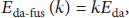$E_{\text{da-fus}}(k)$ expends

$$\begin{array}{cc}& E_{\text{da-fus}}\left(k\right)=k{E}_{\text{da}},\end{array}$$

(4)

where $E_{\text{elec}}$ is energy consumption of sending circuits and receiving circuits. $E_{\text{da}}$ is energy consumption of processing data. ${\epsilon }_{\text{fs}}$ and ${\epsilon }_{\text{mp}}$ are energy consumption of power amplifiers in free space model and multipath fading model, respectively. $d_{\mathrm{0}}$ is threshold of transmission distance.

(2) Objective for Clustering Routing. The objective is to elect K cluster headers from the N sensor nodes to create K clusters, which should meet the following demands: the more the remaining energy in the node is and the closer the distance from the node to the sink node is, the more the possible the node should be a header node. The fitness is designed to be as follows:

$$\begin{array}{cc}& \text{fitness}={\alpha }_{\mathrm{1}}{f}_{\mathrm{1}}+{\alpha }_{\mathrm{2}}{f}_{\mathrm{2}},\end{array}$$

(5)

$\begin{array}{cc}& f_{\mathrm{1}}=\frac{{\sum }_{k=\mathrm{1}}^K{q}_k}{{\sum }_{i=\mathrm{1}}^N{q}_i},\end{array}$

(6)

$\begin{array}{cc}& f_{\mathrm{2}}=\frac{{\sum }_{i=\mathrm{1}}^N{l}_i}{{\sum }_{k=\mathrm{1}}^K{l}_k},\end{array}$

(7)

where ${\alpha }_{\mathrm{1}}$ and ${\alpha }_{\mathrm{2}}$ are weight factors and meet ${\alpha }_{\mathrm{1}}+{\alpha }_{\mathrm{2}}=\mathrm{1}$ .   $q_i$ is the remaining energy of ith node in the network, $q_k$ is the remaining energy of kth cluster header, $f_{\mathrm{1}}$ is an evaluating factor of energy, $l_i$ is the distance from ith node to the sink node, $l_k$ is the distance from kth cluster header to the sink node, and $f_{\mathrm{2}}$ is an evaluating factor of distance.

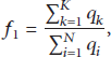
From (5), we can see that the problem of electing K cluster headers from the N sensor nodes becomes to find K candidates to make its fitness optimal, which is a typical optimization problem.

5.2.2. Creation of Life's Living Space

Unlike continuous functions, to select K candidates from N nodes is a problem of discrete event. How to set up a life's living space to use LSE to optimize this kind of problems becomes a critical problem.

Let us first analyse what is a life in the problem. In continuous functions, a life is a point in variable space. But now what are the variables in the cluster routing problem? It is obvious that K different candidates are variables. In other words, each candidate in K candidates could vary from node Number 1 to Number N; thus, each candidate is a variable. By this way, we can create a living space for life, each candidate is its coordinate as follows.

•  

Life's living space = {candidate 1, candidate $2,\dots$ , candidate $K\hspace{0.17em}|\hspace{0.17em}\mathrm{e}\mathrm{a}\mathrm{c}\mathrm{h}$ candidate could take a serial number of nodes from Number 1 to Number $N\}$ .

For example, if we select 2 cluster headers in the 100 nodes that are randomly distributed in an interesting area, we can firstly give each node a serial number from Number 1 to Number 100 according to a certain order, as shown in Figure 5. The living space could be set up afterwards as shown in Figure 6, which is a discrete two-dimensional space.

Figure 5

100 nodes randomly distributed in an interesting area.

Figure 6

Discrete two-dimensional living space.

In Figure 6, the possible value of candidate 1 is the serial number from Number 1 to Number 100, while the possible value of candidate 2 is also the serial number from Number 1 to Number 100 too, where the serial number represents the node of the number. It is obvious that these two candidates cannot be allowed to be the same node, so the positions marked by black cycle could not be any life's position, whereas the positions marked by yellow cycle make up life's living space which is a two-dimensional living space, as shown in Figure 6. In this living space, any life located at positions marked by yellow cycle represents both candidate 1 and candidate 2 that are two possible candidate cluster headers indicated with the serial number. In other words, the values of coordinate axes x and y in the two-dimensional living space should be the serial number of the nodes in the sensing area, where a life has two coordinates, x and y, which are discrete values.

From the analysis mentioned above, the following conclusion could be drawn. If we select K candidates from N nodes, the life's living space is a k-dimensional space.

5.2.3. Application of LSE to Discrete Living Space

After setting up the life's living space, the next problem is how to apply LSE to optimize the living space. In fact, it becomes an easy problem compared with the continuous functions optimization; the only difference is that the values of the coordinate axes x and y are discrete ones instead of continuous ones in LSE.

For example, in the discrete two-dimensional living space shown in Figure 6, the values of coordinate axes x and y fall into $\{\mathrm{1,2},\dots ,\mathrm{100}\}$ with lower bound 1 and upper bound 100, where LSE is easy to be used.

5.2.4. Clustering Routing Algorithm Based on LSE

Clustering routing algorithm based on LSE is described in Algorithm 3.

Algorithm 3: Clustering routing algorithm based on LSE.

Step  1. Initialization.

   Set the number of nodes in initial sensor networks;

   Set the parameters of energy model according to (2), (3) and (4);

   Set the parameters of fitness according to (5);

   Set the maximum number of data transmission;

Step  2. Select cluster heads, set up clusters, create schedule and then transmit data according to the methods provided by LEACH;

Step  3. Judge whether the maximum number of data transmission is reached. If reached, go to Step  7;

Step  4. Cluster head selection optimized by LSE:

Step  4.1. Give a serial number to each node in the interesting area;

Step  4.2. Set the number of cluster heads;

Step  4.3. Set the maximum number of iterations according to computing capability of each node;

Step  4.4. Judge whether the maximum number of iterations is reached. If reached, go to Step  5;

Step  4.5. Optimization by LSE according to Sections 5.2.2 and 5.2.3, where fitness is computed by (5);

Step  4.6. Issue the information of cluster headers;

Step  4.7. go to Step  4.4;

Step  5. Set up clusters, create schedule and then transmit data according to the methods provided by LEACH;

Step  6. Goto Step  3

Step  7. End

In the first round, at the beginning of deployment, the remaining energy of all the nodes in the sensor networks is provided to be equivalent. Therefore, we can still employ LEACH algorithm for the selection of cluster heads as shown in Step 2. From the second round, the remaining energy of all the nodes in the sensor networks is no longer equivalent, and the sink node should use the optimization methods based on LSE introduced in the paper for the selection of cluster heads as shown in Step 4.

In Step 4.5, the process of cluster head selection optimized by LSE should be done according to the methods described previously in Sections 5.2.2 and 5.2.3.

In Section 5.2, LSE is used as an optimization tool for routing protocol in wireless sensor network and its optimization methods and processes are described in detail, by which we can see that LSE is also applicable for the optimization for some discrete problems in real world.

6. Conclusions

In this paper, a new computational intelligence approach, namely, living space evolution (LSE), is presented, which is inspired by life cycle and survival of the fittest and combined with the consideration of living space information. LSE dynamic model, its flow, and pseudocodes are described in detail. A digital simulation has shown the procedure of LSE. Furthermore, two applications of using LSE are employed to demonstrate its effectiveness and applicability. One is to apply it to the optimization for continuous functions; the other is to use it as an optimization tool for routing protocol in wireless sensor network that is a discrete problem in real world.

By means of simulations and discussions in the paper, conclusions could be summarized as follows.

(1) Research has shown that LSE is effective for the optimization for the continuous functions and also applicable for the discrete problem in real world.

(2) LSE has reflected two new ideas. One is living space evolution. The other is multiple offspring reproduction. Multiple offspring reproduction is the prerequisite and guarantee for achieving living space evolution.

(3) The critical question for LSE's applications is the creation of living space. For continuous function, living space is its variable space. But, for discrete problem in real world, how to create its living space depends on specific issues.

(4) In LSE, its prophase is exploration and its anaphase is exploitation; in other words, LSE has a special ability to balance search process from exploration to exploitation gradually.