A Parallel High Speed Lossless Data Compression Algorithm in Large-Scale Wireless Sensor Network

Abstract

In large-scale wireless sensor networks, massive sensor data generated by a large number of sensor nodes call for being stored and disposed. Though limited by the energy and bandwidth, a large-scale wireless sensor network displays the disadvantages of fusing the data collected by the sensor nodes and compressing them at the sensor nodes. Thus the goals of reduction of bandwidth and a high speed of data processing should be achieved at the second-level sink nodes. Traditional compression technology is unable to appropriately meet the demands of processing massive sensor data with a high compression rate and low energy cost. In this paper, Parallel Matching Lempel-Ziv-Storer-Szymanski (PMLZSS), a high speed lossless data compression algorithm, making use of the CUDA framework at the second-level sink node is presented. The core idea of PMLZSS algorithm is parallel matrix matching. PMLZSS algorithm divides the data compression files into multiple compressed dictionary window strings and prereading window strings along the vertical and horizontal axes of the matrices, respectively. All of the matrices are parallel matched in the different thread blocks. Compared with LZSS and BZIP2 on the traditional serial CPU platforms, the compression speed of PMLZSS increases about 16 times while, for BZIP2, the compression speed increases about 12 times when the basic compression rate unchanged.

1. Introduction

With the increasing in the production and propagation of data carriers, such as computers, intelligent mobile phones, and sensing equipment, the data growth of the whole world has increased rapidly and there are also various data types. The total amount of information in the world has doubled every two years in the last 10 years; the total amount of data established and duplicated was 1.8 ZB in 2011 and will be 8 ZB in the near future. Furthermore, it will be 50 times in the next 10 years according to International Data Corp. Three kinds of dominant data types are transactional data, represented by electronic business, interactive data, represented by social networks, and wireless sensor data represented by wireless sensor networks (WSNs). These types occupy 80% to 90% of the total data. The growth rate of unstructured data is much higher than that of structured data [1].

WSNs are considered as one of the most important technologies in the new century. They connect the Internet through a large number of wireless sensors and MEMS (microelectromechanical systems), thus becoming a bridge between the real world and the virtual world of the network. They also allow real world objects to be perceived, recognized, and managed, thus providing the information on the physical environment and other related data for people directly, effectively, and genuinely.

In terms of the large scale of a WSN, there are two main points: first, the sensors can be distributed in a vast geographical area, such as a large number of sensor nodes deployed in a large environmental monitoring area, and second, a large number of sensor nodes can be densely deployed in a small geographical area to obtain the precise data.

Since the Smart Earth plan proposed by USA, the large-scale wireless sensor network (LSWSN) has become an important factor in the comprehensive national strength contest. The new LSWSNs have been listed as a crucial technology in the economy and national security of America. Furthermore they are a key research field in UK, Germany, Canada, Finland, Italy, Japan, South Korea, and the European Union [2].

As a new technology for acquiring and processing information, LSWSNs have been widely used in military and civilian fields.

LSWSN has the characteristics of rapid deployment, good concealment, and high fault tolerance, making it suitable for some applications in the military field. The wireless sensors can be scattered into the enemy military positions through air delivery and long-range projectiles. Those sensors will deploy a self-organizing WSN to secretly collect real-time information in the battlefield at close range [3].

It is also more widely used in civilian fields, such as environmental monitoring and forecasting, medical care, intelligent buildings, smart homes, structural health monitoring, urban city traffic information monitoring, large workshop and warehouse management, safety monitoring of airports, and large industrial parks [4–8].

According to Forrester, the ratio of the number of transactions of the Internet of Things to the business of the Internet will be 30 : 1 in 2020 due to the application and popularization of LSWSNs [9].

However, the application of LSWSNs has encountered many challenges in their rapid development process. For example, on the one hand, a large number of redundant data are generated by sensor nodes whose forwarding between the nodes causes a lot of energy to be wasted at the nodes and the delay of network transmission; on the other hand, as shown in Figure 1, the second-level sink node centralizes massive sensor data from the first-level sink node, seriously affecting the responses of the application layer. This series of problems undoubtedly restrict the further development of LSWSNs.

Figure 1

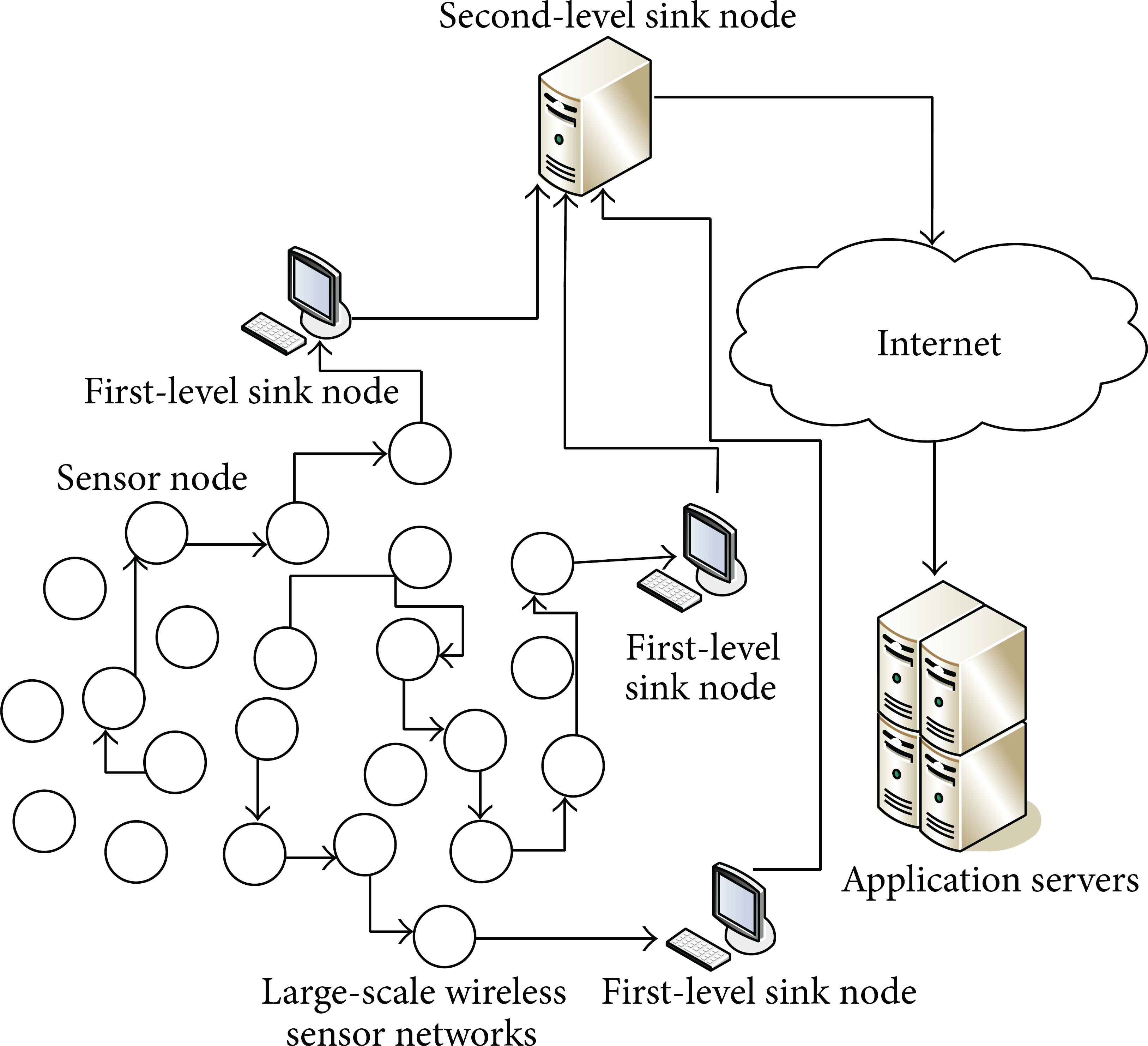
The organizational structure of a large-scale wireless sensor network.

According to the characteristics of the LSWSN, the research focuses on two aspects.

• (a)

The Data Compression Algorithm at the Sensor Nodes. The algorithm reduces the transmission of redundant data, causing less energy wastage and thus lengthening the service life of the LSWSN. The study [10] shows that the energy consumption of data communication is much higher than that of data operation at sensor nodes, as the energy required to transmit one bit is about 480 times that of executing one addition operation. Some data compression schemes of sensor nodes have been proposed, such as the lifting wavelet transform for wireless sensor networks [11], the coding-by-ordering data compression scheme [12].

(b)

The Massive Sensor Data Compression Algorithm at the Second-Level Sink Node. The algorithm improves the transmission bandwidth utilization and increases the processing speed of massive sensor data storage. The LSWSN, which consists of a large number of nodes, is connected with and integrated into the dynamic network. Meanwhile a large number of nodes in the network carrying out real-time data collection and information interaction have produced massive sensor data to be stored and processed. As shown in Figure 1, massive sensor data would finally converge at the second-level sink node and would then be transmitted to the remote servers to be calculated and processed through the network. Then the data preprocessing at the second-level sink node affects the value of application of the LSWSN [13–15]. Therefore, study of the compression of massive sensor data in networks is a hot topic in the field of wireless sensor networks.

In fact, the current research on sensor networks mainly adopts lightweight processing nodes as sensor nodes and sink nodes. The calculation abilities of sink nodes do not meet the performance demand of massive sensor data compression by traditional algorithms. Ohara et al. [16] introduced multicore processors as sensor nodes for wireless sensor networks for special purposes. But, for sink nodes, the calculation ability is still not satisfactory. All of these factors are due to the characteristics of the CPU design. Most of the transistors in the CPU are used for cache and logic control, and only a small part are used for calculation for speeding up a single thread of execution. It is not possible to run hundreds of threads in parallel on CPU.

But the design intent of a GPU [17] is not the same as that of a CPU. A large number of transistors are used in the data execution units such as the processor array, multithreads management, and shared memory. However only a small number of transistors are used by the control units. Contrary to those of CPU, the performance and execution time of a single thread of the GPU lead to the improvement of the overall performance of GPU. Meanwhile thousands of threads are executed on the GPU in parallel and a very high memory bandwidth between threads is provided. GPU has a distinct advantage over CPU in dealing with parallel computing without data association and interaction between threads.

In this work, we study the challenges of a parallel compression algorithm implemented on a CPU and a GPU hybrid platform at the second-level sink node of the LSWSN. As the matrix matching principle introduced, it divides the compressed data into multiple dictionary strings and preread strings dynamically along the vertical and horizontal axes in the different blocks of the GPU and then it forms multiple matrices in parallel. By taking advantage of the high parallel performance of the GPU in this model, it carries out the data-intensive computing of the LSWSN data compression on the GPU. Furthermore it allocates threads’ work reasonably through careful calculation, storing the match result of each block in the corresponding shared memory. Thus it is possible to achieve a great reduction of the fetch time. At the same time, the branching code is avoided as far as possible. Our implementation makes it possible for the GPU to become a compression coprocessor, lightening the processing burden of the CPU by using GPU cycles. Many benefits are shown through the above measures: the less energy consumption of intercommunication and more importantly the less time spending in finding the redundant data, thus speeding up the data compression. It supports efficient data compression with minimal cost compared with the traditional CPU computing platform at the second-level sink node of the LSWSN. The algorithm increases the average compression speed nearly 16 times compared with the CPU mode on the premise that the compression ratio remains the same.

The paper is organized as follows. Section 2 reviews the related works. Section 3 introduces the LZSS algorithm and BF algorithm. Then the parallel high-speed lossless compression is accounted based on the parallel matching LZSS (PMLZSS) algorithm in LSWSN and our implementation details are put forward in Section 4. The experiments and analysis of results are presented in Section 5, and finally Section 6 concludes the paper.

2. Related Works

Sensor node data compression technology is adopted to study how to effectively reduce data redundancy and to reduce the data transmission quantity at sensor nodes without losing the data precision.

Most of the existing data compression algorithms are not feasible for LSWSN. One reason is the size of the algorithm; another reason is the processor speed [10]. Thus, it is necessary to design a low-complexity and small-size data compression algorithm for the sensor network.

Wavelet compression technology has evolved on the basic theory of wavelet analysis and wavelet transform. The core idea presents that most energy of one data series is centered on partial coefficients through the wavelet transform, when another part of the coefficient is set to 0 or approximately 0. Then small parts of the important coefficients are maintained by the certain coefficient decision algorithm. Finally the approximate data sequences of the original data are reconstructed by taking the inverse wavelet transform of the small important coefficients when the original data sequence is needed.

Haar Wavelet Data Compression algorithm with Error Bound (HWDC-EB) for wireless sensor networks was proposed by Zhang et al. [18] based on the wavelet transform, which simultaneously explored the temporal and multiple-streams correlations among the sensor data. The temporal correlation in one stream was captured by the one-dimensional Haar wavelet transform.

Ciancio et al. [19] proposed the Distributed Wavelet Compression (DWC) algorithm, which extracted the spatial-temporal correlation of sensing data before transmitting to the next node through the interaction of pieces of information with each other among the closed sensor nodes. Although the algorithm greatly reduces the transmission of redundant data, the whole complicated processing leads to serious network time-delay.

For the local less jitter and time sequence data, Keogh proposed the Piecewise Constant Approximation (PCA) algorithm [20], whose basic idea was to segment long time sequence data; then, every segment could be represented by the data mean constant and end position mark. Then the Poor Man Mean Compression (PMC) algorithm put forward by Lazaridis and Mehrotra [21] made best use of the mean data in each subsegment of the data sequence as the approximation constant to replace the subsegment. But the compression algorithm based on the subsegment is lack of a global view as only a data sequence is concerned within the current continuous time.

With the massive data increasingly produced by the LSWSN in the application process, the difficulties of data storage and process arise, seriously affecting the large-scale use of the LSWSN. To solve the problem, the sensor data should be compressed at the second-level sink node before being transmitted to the remote servers via the network. For massive data compression, the big problem lies in how to perform the compression quickly in a certain period of time. However the present compression algorithms are required to go through compression processing on the basis of full serial analysis of the raw data, which leads to low speed and low compression efficiency for massive sensor data. In view of the present situation, the key question is how to implement parallel compression based on the existing compression algorithms in order to solve the problems.

Data compression can be classified as lossy compression and lossless compression according to basic information theory [22].

Lossy compression compresses the redundancy of the input data and the information it contains, but some information is lost.

Lossless compression compresses the redundant information of the input data, and the information is not lost in the compression process.

Lossless compression can be divided into two different modes: stream compression mode and block compression mode. The block compression mode divides the data into different blocks according to a certain policy and then compresses each block separately. The classic compression algorithms such as Prediction by Partial Matching (PPM), Burrows-Wheeler Transform (BWT), Lempel-Ziv-Storer-Szymanski (LZSS), Lempel-Ziv-Welch (LZW), and Block Huffman Coding (BHC) all take advantage of block compression.

Gilchrist proposed the BZIP2 algorithm [23] with multithreads, whose core idea was to chunk the data into blocks, with different threads completing compression tasks in each block, respectively. GZIP took advantage of the multicore technology to compress data and Pradhan et al. [24] introduced the distributed computing technique to improve the performance of data compression. All of these improvements are achieved by optimization algorithms confined to the CPU platform. But the improvement of the performance is limited by the number of multithreads running concurrently and the number of communication data among the multithreads on the CPU platform.

Since the advent of GPU, some scholars have also done a lot of work on data compression. Many lossy compression algorithms based on GPU are successful, such as the use of GPUs to speed up the execution time of JPEG2000 image compression [25] and the use of GPUs to compress space applications data [26]. Recently, this has been a hot research topic for improving the performance of lossless data compression algorithms based on GPUs. Taking the image compression field as an example, many improvements in image compression and transmission performance have been made by GPU. O'Neil and Burtscher [27] proposed a parallel compression algorithm based on a GPU platform specifically for double precision floating point data (GFC), whose compression speed was raised by about two orders of magnitude compared with BZIP2 and GZIP running on the CPU platform.

Although RLE is not a very parallelizable algorithm, Lietsch and Marquardt [28] and Fang et al. [29] took advantage of the shared memory and global memory of the GPU to improve it. But the acceleration effect was not very obvious in practice. Cloud et al. [30] and Patel et al. [31] improved the classic BZIP2 algorithm; their basic ideas were to make use of the block compression and to improve the parallel code fit for the GPU, mainly in the three stages of the algorithm: the Burrows-Wheeler Transforms (BWT), Move-To-Front (MTF), and Human Coding.

In most of the above studies, the data are chunked into blocks directly, and then the blocks are processed in parallel. Data dependencies exist if we only chunk the data simply. The acceleration effect is not ideal in practical applications. Thus the emphasis of our work is to focus on how to find inherent parallelism in compression algorithms and how to transplant them to the GPU platform.

3. LZSS Algorithm and BF Algorithm

The LZSS algorithm [32], a widely used data compression algorithm and being a CPU-based serial algorithm, is not suitable for GPU architecture. The BF algorithm is a serial string matching algorithm, although its time complexity is $O(m*n)$ . However, compared to KMP, BM, and BOM algorithm, it can be easily converted from the serial computing model to the parallel computing model after modification.

3.1. LZSS Algorithm

LZSS is an improvement of LZ77 [33]. First, it establishes a binary search tree, and second, it changes the structure of the output encoding, which solves the problem of LZ77 effectively. The standard LZSS algorithm uses a dynamic dictionary window which is 4 KB and a prereading window to store the uncompressed data whose buffer size is usually between 1 and 256 bytes. The basic idea of LZSS is to find the longest match of the prereading window in the dictionary window dynamically. The output of the algorithm will be a two-tuple (offset, size) if the length of the matching data is longer than the minimum matching length. Otherwise the output will be the original data directly.

For example, for the raw data AABBCBBAABCAC, it outputs the result AABBC(3, 2)(7, 3)CAC using the LZSS compression processing. The dictionary window and the prereading window slide back once every time a datum is processed to repeatedly deal with the rest of the data.

When coding in practice, LZSS combines the compressed coding and raw data to improve the ratio of compression. Each byte has a one-bit identifier and consecutive eight-bit identifiers, which constitute a flag byte. The output format is one flag byte and eight data bytes continuously, which indicates the original data when the identifier bit is 0 and compressed data when it is 1.

3.2. Basic Serial BF String Matching Algorithm

For the object string and pattern string, the serial BF string matching algorithm matches the pattern string from the start of the object string to compare object $[0]$ with pattern $[0]$ . If they are equal, it continues to compare subsequent characters and the match is successful if all of the characters are the same. Otherwise the pattern string goes back to the start position and the object string goes back to the start+1 position to continue comparing.

The pseudocode is referred to as Algorithm 1.

Algorithm 1

 Algorithm  1

 BFStringMatch (char^*Object, char^*Pattern) {

 int len_T = strlen(Object); int len_P = strlen(Pattern);

  for (int i = 0; i <= len_T-len_P; i++){

   int j = 0; k = i; // find the matching string of Pattern string from i position in Object string

   while (j < len_P && Object[k] == Pattern[j]) {k++, j++}

    if (j == m) // find a matching substring, record the position

     Object string forward one byte to find the next match;

 }

}

4. Implementation of Lossless Compression Based on Parallel Matching LZSS at Sink Node

The architecture of the GPU is Single Instruction Multiple Thread (SIMT), which is very suitable for handling repetitive character matching. It converts the serial computing model of the original BF algorithm to the parallel computing model and supplements the LZSS compression algorithm with the BF algorithm. Thus an efficient parallel lossless compression algorithm based on GPU and CPU platforms at the second-level sink node is described in this section.

With regard to improving the compression ratio, the speed of the compression is improved slowly [34] for the latest relevant research on the LZSS algorithm. The key to the compression speed is to speed up the matching of the two strings in the two dynamic sliding windows through the analysis of the LZSS algorithm.

BF is a typical serial algorithm according to the analysis in Section 3.2, which matches the strings using two layers of loops. The inner loop judges whether the string whose length is equal to the length of the pattern string in the dictionary window matches the pattern string, and the outer layer is used to move the dictionary window. The process of searching for pattern string matching in the object string is completely independent, which provides an opportunity to convert BF into a parallel algorithm on the GPU platform.

GPU supports a large number of threads running concurrently. If one GPU thread corresponds to one match of the compressing data, with regard to the 4 KB compression dictionary window in the LZSS algorithm, 4096 GPU threads should be run. It is no problem for the GPU to run 4096 or even higher order of magnitude of threads concurrently. Although running several threads in parallel does not work for the general program development of the actual GPU, it is necessary to deal with more practical questions. GPU is inefficient for branch operation because it is not suitable for logic control. During the task running process, different data leads to different thread speeds executing different subtasks. In the execution of such a task scheduling, the execution time of the slowest threads will decide the whole task execution time.

In accordance with the features of GPU, the expensive calculations of the task are accelerated in parallel on GPU, and the serial parts of the task are preperformed on CPU. In principle, the above has stated that on the one hand the tasks of matching the dictionary strings with several prereading window strings are implemented on GPU, which achieve acceleration of the parallelization. On the other hand, the serial operations such as matching result synthesis and data compression are implemented on CPU.

4.1. The Improved Flag Byte

In LZSS, in order to combine the compression coding and the raw data, a flag byte is set every 8 data bytes. Negative compression would occur if fewer data could be compressed in a file. In this paper two categories of flag bytes are set: the mixed flag byte and the original flag byte. The first bit of the mixed flag byte is 1, and the other 7 bits are marked as 7 mixed data bytes. The first bit of the original flag byte is 0 and it outputs 128 raw data bytes consecutively at the most. It greatly reduces the number of flag bytes to increase the compression ratio. The output of the above raw string is (0001001)AABBC(11111000)(3, 2)(7, 3)CAC.

4.2. Setting the Length of the Dictionary Window

The length of the dictionary window is set as long as possible to discover more compressible data, but it also brings the problem of the expansion of search range. The length of the offset of the matching data relative to the dictionary window becomes longer. Two bits are used to represent the offset in the mixed flag byte, making the maximum length of the dictionary window up to 64 KB.

4.3. PMLZSS Parallel Matching Model

Each thread has to frequently access the global memory via the general parallel matching algorithm, thus reducing the compression performance. In the CUDA environment, each thread has its own shared memory, and all the data in the shared memory are accessed directly for all the threads in the same block. Making use of the high parallel of GPU, combining the advantages of LZSS algorithm and BF algorithm, the PMLZSS speeds up the data compression.

As shown in Figure 2, using the idea of LZSS for reference, the PMLZSS algorithm divides the data compression file into two parts: the compressed dictionary window and the prereading window. The lengths of the two windows are cKB and $16*n$ B, respectively. In order to make full use of GPU parallel processing capabilities, the data compression file should be divided into several pairs of compressed dictionary windows and prereading windows, not just one pair as in LZSS.

Figure 2

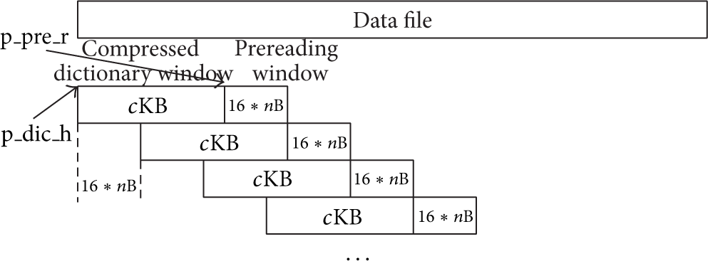
Division of the data file into multiple pairs of compressed dictionary windows and prereading windows.

As shown in Figure 3, it builds up a matrix where the data in the compressed dictionary window in bytes is shown on the vertical axis and the data in the prereading window in bytes is shown on the horizontal axis.

Figure 3

The matrix matching by a pair of a compressed dictionary window and a prereading window.

After studying the BF algorithm, PMLZSS adopts the violence matching method to perform parallel matching so that for each byte on the vertical axis one thread should be invoked to match all bytes on the corresponding horizontal axis (i.e., the bytes in the corresponding prereading window). If it finds a match, the position in the matrix will be set to 1; otherwise it will be set to 0.

Finally, it finds the longest oblique line segment with consecutive 1 s through the whole matrix, recording the start and end positions, and the length of the oblique line segment, sending them into the CPU as parameters for data compression.

4.4. PMLZSS Algorithm Implementation

According to the parallel matching model, the specific data parallel compression process entailed the following steps:

• (1)

reading the data compression file and then copying this file from memory to the global memory of GPU;

(2)

setting the thread block groups on GPU as $blk[a]$ , in which a is the total number of thread blocks and the number of threads in each block is b;

(3)

setting the length of the compressed dictionary window as cB and setting the pointer to the first compressed dictionary window as $p\_dic\_h$ , whose initial value points to the beginning of the data compression file;

(4)

setting the size of the prereading window as d and setting the pointer to the first prereading window as $p\_pre\_r$ , whose initial value is $p\_dic\_h\text{-}c$ ;

(5)

initializing the thread group $threads[a*b]$ and $(a*b/\mathrm{2})/c\mathrm{\hspace{0.17em}\hspace{0.17em}}gMatrix$ matrices, whose size is $c*d$ ;

(6)

invoking $(a*b/\mathrm{2})$ threads in the thread group $threads[a*b]$ to deal with $q=(a*b/\mathrm{2})/c$ data segments in the data compression file, whose length is $c+d$ . The compressed dictionary windows and the corresponding prereading windows are shown in Figure 2. $p\_dic\_h$ points to the header of the 0th compressed dictionary window, $p\_pre\_r$ points to the header of the 0th prereading window, $p\_dic\_h+d$ points to the header of the 1st compressed dictionary window, $p\_pre\_r+d$ points to the header of the 1st prereading window, and so on. q pairs of a compressed dictionary window and a prereading window can be dealt with in a cycle.

 

Specifically, for the data in each compressed dictionary window and corresponding prereading window, the algorithm performs the following steps respectively,

• (6-1)

setting the counter $i=\mathrm{0}$ ;

(6-2)

setting thread $T_{\mathrm{1}}$ , whose thread number is $th\mathrm{1}$ and then using thread $T_{\mathrm{1}}$ to judge whether the $(th\mathrm{1}\mathrm{\hspace{0.17em}\hspace{0.17em}}mod\mathrm{\hspace{0.17em}\hspace{0.17em}}c)$ th byte in the kth compressed dictionary window matches the bytes from the $(i*\mathrm{16})$ th to the $((i+\mathrm{1})*\mathrm{16}-\mathrm{1})$ th byte in the kth prereading window (i.e., whether the two bytes are equal), where $\mathrm{0}\le k<q$ . It returns 1 if the two bytes match and 0 otherwise. Then the results are written back to the global memory in the kth $gMatrix$ matrix from position $((th\mathrm{1}\mathrm{\hspace{0.17em}\hspace{0.17em}}mod\mathrm{\hspace{0.17em}\hspace{0.17em}}c)*d+i*\mathrm{16})$ to position $((th\mathrm{1}\mathrm{\hspace{0.17em}\hspace{0.17em}}mod\mathrm{\hspace{0.17em}\hspace{0.17em}}c)*d+i*\mathrm{16}+\mathrm{16})$ ;

(6-3)

$i++$ , return to (6-2) when $i<n$ ; otherwise go to (7);

(7)

Finding the longest oblique line segment with consecutive 1 s in the q results matrices $gMatrix$ , determining the result triads array $locations[p]$ , whose element has stored three components, which were (x, y, $length$ ). This shows that a match is not found when the $length$ is less than 3 (if the length of the matching substring is less than 3 bytes, the length of the compressed code would be longer than the raw data), and x and y are set to $-\mathrm{1}$ directly for meaningless;

 

This step includes the following substeps:

• (7-1)

setting thread $T_{\mathrm{2}}$ , whose number is $th\mathrm{2}$ and then using $T_{\mathrm{2}}$ to find the longest oblique line segment with consecutive 1 s, recording its corresponding parameters x, y, and $length$ ;

(7-2)

thread that $T_{\mathrm{2}}$ gets the corresponding data of x, y, and $length$ and then stores them in the element of the result triads array $locations$ whose index is $(th\mathrm{2}\mathrm{\hspace{0.17em}\hspace{0.17em}}mod\mathrm{\hspace{0.17em}\hspace{0.17em}}p)$ ;

(8)

finding the element that has the maximum value of $length$ . Setting thread $T_{\mathrm{3}}$ , whose number is $th\mathrm{3}$ , using $T_{\mathrm{3}}$ to find the element that has the maximum value of $length$ in the corresponding array $locations$ of each $gMatrix$ , and storing them in the global match result array $match[q]$ . The elements of this array store the results triad (x, y, $length$ );

(9)

compressing the data according to the matching results array $match[q]$ , including the following steps:

• (9-1)

copying the matching result array $match[q]$ from the GPU to the memory of CPU;

(9-2)

conversion by CPU of the data stored in the matching result array $match[q]$ into the $offset$ of the longest match and the $length$ of the substring of the prereading window in the compressed dictionary window and outputting of the triple compression code array $compress[q]$ . The elements of this array store the results triad ( $flag$ , $offset$ , $length$ );

(9-3)

compression of the data by CPU according to the $flag$ ;

(10)

determining whether the pointer $p\_pre\_r$ has pointed to the end of the data compression file: the process is finished if the pointer has pointed to the end of the data compression file. Otherwise the algorithm slides the dictionary windows and prereading windows forward, that is, setting $p\_pre\_r=p\_pre\_r+q*d$ and $p\_dic\_h=p\_dic\_h+q*d$ , and then returns to (6).

4.5. Example of PMLZSS

Setting the data at the beginning of 4096 bytes of the compression file as “ $hellothisaeybc\dots isa$ ,” the data of the following 16 bytes were “ $thisisaexampletosh$ .”

According to the above PMLZSS algorithm process, the steps are as follows:

• (1)

CPU that reads the data compression file and then copies this file from memory to the global memory of GPU;

(2)

setting the thread block groups on GPU as $blk[1024]$ and then the number of threads in each thread block is 512;

(3)

setting the length of the compressed dictionary window as 4096 B, while the pointer to the first compressed dictionary window is $p\_dic\_h=0$ ;

(4)

setting the size of the prereading window as 64 B and the pointer to the first prereading window as $p\_pre\_r=4096$ ;

(5)

initializing the thread group $threads[1024*512]$ and 64 $gMatrix$ matrixes, whose size is 4096 * 64;

(6)

invoking 1024 * 256 threads in the thread group $threads[1024*512]$ to deal with 64 data segments in the data compression file, whose lengths are $(4096+64)$ bytes.

 

As shown in Figure 4, the resources below describe the processing work of the 0th compressed dictionary window and the corresponding prereading window in detail.

 

From $T_0$ to $T_{4095}$ , altogether 4096 threads are in a thread group, and the thread numbers are 0 to 4095, respectively. $T_{m1}$ ( $m1\in [\mathrm{0,4095}]$ ) is one of the threads whose thread number is $m1$ . It is responsible for judging whether the $m1$ th byte in the compressed dictionary window matches the bytes from the 0th to the 15th byte in the prereading window (i.e., whether the two bytes are equal). It will return a value of 1 when the two bytes are matched; otherwise it will return a value of 0. Then the results are written back to the position $m1*64$ to $m1*64+16$ of the corresponding $gMatrix$ matrix in the global memory. When 16 bytes of data are compressed, a loop is executed with $i=0$ and the result is 4096 * 16, which is a quarter of one $gMatrix$ ;

(7)

as shown in Figure 5, the example uses the 0th $gMatrix$ to describe the process of finding the longest oblique line segment with consecutive 1 s;

 

from $T_0$ to $T_{4110}$ , all $(4096+15)$ threads are in a thread group. The thread numbers are 0 to 4110, respectively. $T_{m2}$ ( $m2\in [\mathrm{0,4110}]$ ) is one of the threads whose thread number is $m2$ and is responsible for finding the longest subsegment in the oblique line segment with consecutive 1 s.

 

$T_{m2}$ will get the parameters x, y, and $length$ and store them in the $m2$ element of the triplet result array $locations$ .

 

As seen in Figure 6, thread $T_5$ and thread $T_{10}$ find multiple lines of consecutive 1 s, and their corresponding element values are in the $locations$ : $locations[5]=\{\mathrm{5,0},6\}$ and $locations[10]=\{\mathrm{10,2},3\}$ , while the other element values in the $locations$ are $\{-1,-\mathrm{1,0}\}$ .

(8)

From $T_0$ to $T_{63}$ , altogether 64 threads are in a thread group. The thread numbers are 0 to 63, respectively. $T_{m3}$ ( $m3\in [\mathrm{0,63}]$ ) is one of the threads whose thread number is $m3$ and is responsible for finding the element that has the maximum value of $length$ in the 0th $gMatrix$ corresponding to the $locations$ array and storing the corresponding parameters x, y, and $length$ in the global matching result array $match[64]$ .

 

In this case, the element that has the maximum $length$ value is the 5th element in the array $match$ , which is $match[0]=\{\mathrm{5,0},6\}$ .

(9)

Compression of data: first, the $match[64]$ is copied from GPU to CPU; then the data in the $match[64]$ are converted into the $offset$ of the longest match and $length$ of the substring of the prereading window in the corresponding compressed dictionary window. Finally, the compression code triples $compress[64]$ is output, which included three parameters: $flag$ , $offset$ , and $length$ .

 

In this case, $offset$ and $length$ are 5 and 6, respectively. The value of $flag$ is 224 (11100000) and $compress[0]=\{\mathrm{224,5},6\}$ . After being compressed, the first $(4096+16)$ bytes of the data compression file will be output: $\left(01111111\right)hellothisaeybc\dots isa(11100000)56ample(00000100)tosh$ .

 

The first 4096 bytes in the compressed dictionary window cannot be compressed; the data are output originally. The following (11100000) is a mixed $flag$ byte. The two bytes 5 and 6 after the $flag$ are compressed codes, which denote that a substring whose length is 6 bytes of the prereading window is compressed, and the corresponding compressed dictionary is at the $offset$ 5 of the 0th compressed dictionary window. Then 4 bytes of raw data are output. Finally, an original flag byte whose value is 00000100 is output. The raw data following it is the 4 bytes “ $tosh$ .”

(10)

Finally by deciding that the pointer $p\_pre\_r$ has pointed to the end of the data compression file, the compression process finishes.

Figure 4

The matrix matching.

Figure 5

Finding the longest oblique line segment with consecutive 1 s.

Figure 6

Obtaining the results of locations.

4.6. Time Complexity Analysis

Some definitions are as follows.

Definition 1.

For a given algorithm, suppose the scale of the problem is n and $T(n)$ is the frequency function. Then $T(n)$ is the time complexity of the algorithm which represents the running time required when the scale of the problem waiting for a solution is n. When the scale of the problem n is huge, it is almost impossible, and it is not necessary to obtain an accurate $T(n)$ . Therefore, asymptotic time complexity is introduced.

Definition 2.

For the integer $n>0$ , there is a nonnegative function $f(n)$ . If there are an integer $n_0$ and a positive constant c, for any $n\ge n_0$ , then $f(n)\le c*g(n)$ . The $f(n)$ is the asymptotic upper bound, denoted by $f(n)=O(g(n))$ .

Definition 3.

When the scale of the problem n approaches infinity, the asymptotic upper bound of the algorithm time complexity is $T(n)=O(f(n))$ . The $O(f(n))$ is the asymptotic time complexity of the algorithm, or simply the time complexity for short.

The compression algorithm proposed here mainly consists of the following steps:

• (1)

copying the data from CPU to GPU;

(2)

building multiple matrices for the dictionary string and the prereading string concurrently;

(3)

matching multiple matrices concurrently;

(4)

obtaining the triple array from the result matrix;

(5)

merging the triple array;

(6)

copying the triple array back to CPU;

(7)

compression of the data by CPU according to the triple array.

The total time complexity of the algorithm is the sum of the above seven steps:

$$\begin{array}{l}T\left(n\right)=T_1\left(n\right)+T_2\left(n\right)+T_{\mathrm{3}}\left(n\right)+T_{\mathrm{4}}\left(n\right)\\ \hspace{1em}+T_{\mathrm{5}}\left(n\right)+T_{\mathrm{6}}\left(n\right)+T_{\mathrm{7}}\left(n\right).\end{array}$$

(1)

The time complexities of the first, second, fifth, sixth, and seventh steps are constants; that is,

$$\begin{array}{cc}& T_{\mathrm{1}}\left(n\right)=T_{\mathrm{2}}\left(n\right)=T_{\mathrm{5}}\left(n\right)=T_{\mathrm{6}}\left(n\right)=T_{\mathrm{7}}\left(n\right)=O\left(\mathrm{1}\right).\end{array}$$

(2)

For the third step of the algorithm, when the length of the prereading window is m and the length of the source data to be compressed is n, then the 64 matrices whose dimensions are $4096*m$ are processed in one cycle. The total number of loops is $n/(m*64)$ , and the time complexity for the step is

$$\begin{array}{cc}& T_{\mathrm{3}}\left(n\right)=O\left(\frac{n}{\left(m*\mathrm{64}\right)}\right)=O\left(n\right).\end{array}$$

(3)

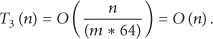
For the fourth step of the algorithm, similar to the third step, 64 matrices whose dimensions are $4096*m$ can be processed in one cycle each time. For multiple threads that are executed concurrently, the time complexity for a single cycle is $O(m)$ . Then the total time complexity for the fourth step is

$$\begin{array}{cc}& T_{\mathrm{4}}\left(n\right)=O\left(\frac{n}{\left(m*\mathrm{64}\right)}\right)=O\left(n\right).\end{array}$$

(4)

The total time complexity of the algorithm is

$$\begin{array}{l}T\left(n\right)=O\left(\mathrm{1}\right)+O\left(\mathrm{1}\right)+O\left(n\right)+O\left(n\right)+O\left(\mathrm{1}\right)\\ \hspace{1em}+O\left(\mathrm{1}\right)+O\left(\mathrm{1}\right)+O\left(\mathrm{1}\right)=O\left(n\right).\end{array}$$

(5)

Thus, the final time complexity of the algorithm is linearly proportional to the length of the source data being compressed.

5. Experiments and Analysis of Results

5.1. Experimental Platform Setting

In order to test the efficiency of the new lossless data compression algorithm PMLZSS on GPU platform in LSWSN, the data compression algorithms BZIP2 and LZSS on CPU platform and the PMLZSS compression algorithm on three different GPU platforms are tested. The four kinds of test platforms at the second-level sink node are as follows:

• (i)

CPU: a six-core Intel Core i7 990x processor running at 3.46 GHz and 24 GB main memory. The operating system is Ubuntu 2.6.32-33, and the compiler is a gcc C compiler 4.4.3;

(ii)

NVIDIA Tesla C2070 GPU, which has 448 cores with 8 streaming multiprocessors running at 1.15 GHz;

(iii)

NVIDIA GTX480 GPUs, which has 480 cores with 15 streaming multiprocessors running at 1.4 GHz;

(iv)

NVIDIA GTX 580 GPUs, which has 512 cores with 16 streaming multiprocessors running at 1.5 GHz.

On GPU platform, the CUDA compiler 4.0 is employed. The communication between CPU and GPU uses a PCIe-x16 whose bandwidth is 6.4 GB/s.

5.2. Test Data Sets

In a large supermarket logistics system supported by the Internet of Things, it is necessary to keep track of location and status information of 50,000,000 items. Assuming that 2,000 times are read every day and that 20 bytes are read each time, then 2 TB is the amount of data generated daily. The sensor data, which amounted to 128 MB in the experiment, is output by the simulation program.

5.3. Experimental Analysis

The BZIP2 algorithm, the original LZSS algorithm, and the PMLZSS algorithm are tested by comparing the data sets. BZIP2 code references [35] and LZSS code references [36] are running on the CPU platform, while the PMLZSS were running on three different GPU platforms, respectively.

Definition 4.

Compression throughput is the total quantity of data handled by the compression procedure per unit time.

Definition 5.

The capacity reduction ratio is the ratio of the difference of the length of data before compression and the length of data after compression to the length of data before compression. The capacity reduction ratio is expressed as a percentage; that is,

$$\begin{array}{l}\text{Capacity}\mathrm{\hspace{0.17em}\hspace{0.17em}}\text{Reduction}\\ =\left(\text{the}\mathrm{\hspace{0.17em}\hspace{0.17em}}\text{length}\mathrm{\hspace{0.17em}\hspace{0.17em}}\text{of}\mathrm{\hspace{0.17em}\hspace{0.17em}}\text{data}\mathrm{\hspace{0.17em}\hspace{0.17em}}\text{before}\mathrm{\hspace{0.17em}\hspace{0.17em}}\text{compression}\right.\\ \phantom{000}-\left.\text{the}\mathrm{\hspace{0.17em}\hspace{0.17em}}\text{length}\mathrm{\hspace{0.17em}\hspace{0.17em}}\text{of}\mathrm{\hspace{0.17em}\hspace{0.17em}}\text{data}\mathrm{\hspace{0.17em}\hspace{0.17em}}\text{after}\mathrm{\hspace{0.17em}\hspace{0.17em}}\text{compression}\right)\\ \hspace{1em}·{\left(\text{the}\mathrm{\hspace{0.17em}\hspace{0.17em}}\text{length}\mathrm{\hspace{0.17em}\hspace{0.17em}}\text{of}\mathrm{\hspace{0.17em}\hspace{0.17em}}\text{data}\mathrm{\hspace{0.17em}\hspace{0.17em}}\text{before}\mathrm{\hspace{0.17em}\hspace{0.17em}}\text{compression}\right)}^{-1}*\mathrm{100}\%.\end{array}$$

(6)

5.3.1. Relationship between the PMLZSS Compression Throughput and the Length of Compression Dictionary Window

The compression throughput of LZSS compression algorithm running on CPU is 28.5 MB/s, while the BZIP2 running on CPU is only 37.35 MB/s, which could not meet the performance requirement of big data compression. When the compression throughput of LZSS is set to 1, the compression throughput speedups of PMLZSS running on the different GPU platforms are shown in Figure 7, whose lengths of prereading windows are set to 64 B, while the lengths of the compression dictionary windows are set to 1 KB, 2 KB, 4 KB, and 8 KB, respectively.

Figure 7

PMLZSS compression speedup.

From Figure 7 the speedup of compression throughput of PMLZSS, which runs on GTX580 while the compression dictionary window is set to be 1 KB, reaches nearly 34 times more than that of LZSS. Furthermore, the speedup of compression throughput reaches 13 times when PMLZSS runs on GPU C2070. Its speedups of compression throughput are in decrease trend with the increase of the lengths of the compression dictionary windows on different GPU platforms. The longer the lengths of the compression dictionary window, the more the calculation of the matching of strings in the prereading window and the compression dictionary window and the lower the speed of compression.

Three factors determining the increase of PMLZSS compression throughput are the numbers of stream processors in a single GPU, the sizes of caches, and the sizes of shared memory in each block of GPU. Therefore, with the development of GPU, the increases of caches, the shared memories, and the number of stream processors in a single GPU chip all account for the improvement of the parallel computing capability. So PMLZSS compression throughput is going upward with it in the expectation.

5.3.2. Relationship between the PMLZSS Capacity Reduction Ratio and the Length of Compression Dictionary Window

PMLZSS capacity reduction ratio is only related to the length of compression dictionary window, having nothing to do with GPU platform as shown in Figure 8. When the length of the compression dictionary window is set smaller, the smaller the possibility of the string in the Prereading Window finding the matching sub-string in the Compression Dictionary Window. Then the less the redundant data, the smaller the capacity reduction ratio and the vice versa.

Figure 8

PMLZSS capacity reduction ratio.

From our research the biggest PMLZSS capacity reduction ratio is only 13.53%, having decreased by nearly 2% compared to LZSS on CPU, far smaller than the BZIP2 on CPU. Moreover it is shown that the LZSS-CPU capacity reduction ratio is only 13.72% and the BZIP2-CPU capacity reduction ratio 22.65% in [37].

The two reasons accounting for the smaller PMLSZZ capacity reduction ratio are as follows.

• (1)

PMLZSS capacity reduction ratio is smaller than that of BZIP2 while PMLZSS focusing on the improvement of compression throughput, not optimizing the related capacity reduction;

(2)

the data unit in the experiment is chunk which is no longer than 64 KB, while the average length is about 10 KB, restraining the increase of capacity reduction ratio to some extent.

5.3.3. Time-Consuming Comparison of PMLZSS at Different Stages

We first test the time cost in various compression stages of the PMLZSS running on three different GPU platforms:

• (1)

MHtoD: the time taken to transmit the data from CPU memory to GPU memory;

(2)

CMatrix: the time taken to construct the matrix in GPU;

(3)

findOne: the time taken to find oblique segments with the greatest number of consecutive 1 s in the matrix on GPU;

(4)

MDtoH: the time taken to transmit the data from GPU memory to CPU memory;

(5)

cpuCompress: the time taken to compress the source data on CPU based on the displacement and the length of data obtained from GPU;

(6)

totaltime: the time taken by the whole compression process.

A subset of the test data set with a size of 128 MB is chosen, and the test is repeated five times. The average time of each stage is indicated in Table 1.

Table 1

The average time of each stage of compression using GPU.

Algorithm	MHtoD (s)	CMatrix (s)	findOne (s)	MDtoH (s)	cpuCompress (s)	Totaltime (s)
PMLZSSC2070	0.0826	3.2173	1.0735	0.0420	0.1203	4.5375
PMLZSSGTX480	0.0702	1.6025	0.9133	0.0381	0.0972	2.7213
PMLZSSGTX580	0.0586	1.1826	0.8142	0.0342	0.0911	2.1807

Table 1 shows that the time costs at the three stages of $MHtoD$ , $MdtoH$ , and $cpuCompree$ are not much different on the three various GPU platforms, while the time cost of $CMatrix$ is very different from the time cost on the PMLZSS-GTX580, which is only just above one-third of that of the PMLZSS-C2070. This is because the GTX580 has more cores, caches, and shared memories, while the frequency of the cores increases. All of this improves the parallel computing ability significantly and should therefore make it possible to create more matrices quickly. At the same time, the time cost of the $findOne$ stage takes almost a quarter of the entire processing time. This should be the spotlight for us in future performance optimization for the reduction of the time taken by this stage.

6. Conclusion

In this paper, we propose a parallel high speed lossless massive data compression algorithm PMLZSS under the framework of CUDA at the second-level sink node of an LSWSN. It introduces a matrix matching process that divides the source data being compressed into multiple dictionary strings and prereading strings dynamically along the horizontal and vertical axes, respectively, in various blocks of GPU, which constructs multiple matrices to match concurrently.

The main aim is to speed up the compression of massive sensor data at the second-level sink node of a LSWSN without decreasing the compression ratio. The tests are performed on a CPU platform and three different GPU platforms. The experimental results show that the compression ratio of PMLZSS decreased by about 2%, compared with the classic serial LZSS algorithm on the CPU platform, and the compression ratio decreases by about 11%, compared with the BZIP2 algorithm, which paid more attention to the compression ratio. But the compression speed of PMLZSS is greatly improved. It is improved by about 16 times compared with the classic serial LZSS algorithm and by nearly 12 times compared with the BZIP2 algorithm. The PMLZSS compression speed is expected to be further improved with the continuous improvements of GPU hardware structure and parallel computing capability.

With the continuous improvement of GPU hardware, especially cache technology and shared memory, a series of problems have also emerged. The first is the cache consistency problem, which needs to use complex logic control that is inconsistent with the GPU hardware design goal; the second is the low hit ratio of the cache. The introduction of caching would slow down reading and writing if the hit ratio of the cache is too low. Last but not least is the cost of the large number of transistors caused by the introduction of the cache. All of these should be considered in the future works.