Minimizing the Number of Mobile Chargers to Keep Large-Scale WRSNs Working Perpetually

Abstract

Wireless Rechargeable Sensor Networks, in which mobile chargers ( $\mathcal{M}\mathcal{C}$ s) are employed to recharge the sensor nodes, have attracted wide attention in recent years. Under proper charging schedules, the $\mathcal{M}\mathcal{C}$ s could keep all the sensor nodes working perpetually. Since $\mathcal{M}\mathcal{C}$ s can be very expensive, this paper tackles the problem of deciding the minimum number of $\mathcal{M}\mathcal{C}$ s and their charging schedules to keep every sensor node working continuously. This problem is NP-hard; we divide it into two subproblems and propose a GCHA (Greedily Construct, Heuristically Assign) scheme to solve them. First, the GCHA greedily addresses a Tour Construction Problem to construct a set of tours to 1-cover the WRSN. Energy of the sensor nodes in each of these tours can be timely replenished by one $\mathcal{M}\mathcal{C}$ according to the decision condition derived from a Greedy Charging Scheme (GCS). Second, the GCHA heuristically solves a Tour Assignment Problem to assign these tours to minimum number of $\mathcal{M}\mathcal{C}$ s. Then each of the $\mathcal{M}\mathcal{C}$ s can apply the GCS to charge along its assigned tours. Simulation results show that, on average, the number of $\mathcal{M}\mathcal{C}$ s obtained by the GCHA scheme is less than 1.1 over a derived lower bound and less than 0.5 over related work.

1. Introduction

During the past decades, Wireless Sensor Networks (WSNs) have been the focus of the research community. WSNs can be widely used in scientific and military data gathering, environmental surveillance, targets monitoring and tracking, and health care, among others. WSNs are composed of many small-sized sensor nodes. Due to cost and size limitations, however, the battery volume of each sensor node is very small. Therefore, energy problem poses a barrier for large-scale deployment of WSNs. To prolong the lifespan of WSNs, methods of energy conservation [1], incremental deployment [2], energy harvesting [3], and wireless charging are proposed. Among these methods, wireless charging is the most promising in removing the energy bottleneck of WSNs [4]. By applying the technique of wireless charging, which refers to magnetic resonant coupling [5] in this paper, a new paradigm of Wireless Rechargeable Sensor Networks (WRSNs) is proposed and immediately received wide attention. In WRSNs, mobile chargers ( $\mathcal{M}\mathcal{C}$ s) with high volume batteries are employed to replenish the depleted energy of rechargeable sensor nodes. The batteries of the $\mathcal{M}\mathcal{C}$ s can be quickly renewed at a service station ( $\mathcal{S}$ ). In this way, lifespan of WRSNs can be significantly prolonged, or theoretically speaking, to infinity. Applications include sustainable WRSNs in smart grids [6] and underground sensor networks powered by UAVs [7].

Most existing works on WRSNs only use one $\mathcal{M}\mathcal{C}$ to conduct charging. However, an open issue in these works is their poor scalability. Even when the $\mathcal{M}\mathcal{C}$ can simultaneously charge all sensor nodes within its charging area, the maximum network size is still limited by its charging power, moving speed, and total energy. Therefore, multiple $\mathcal{M}\mathcal{C}$ s are employed to address the problem.

Since an $\mathcal{M}\mathcal{C}$ can be very expensive, the first and foremost issue in designing a WRSN with multiple $\mathcal{M}\mathcal{C}$ s is to decide the minimum number of $\mathcal{M}\mathcal{C}$ s required, so that no sensor node will die. This problem, named Minimum Mobile Chargers Problem (MMCP) [8], is closely related to the Distance-Constrained Vehicle Routing Problem (DVRP) [9]. Given a network $G=(E,V)$ and a distance bound D, the DVRP [9] is to find a minimum cardinality set of tours originating from a depot that covers all the vertices in V. Each tour is required to have length at most D. Since $\mathcal{M}\mathcal{C}$ s are also energy-constrained, researchers reduce MMCP to DVRP, so that solutions for DVRP can be applied to address MMCP [8]. We, however, argue that DVRP is only a subproblem of MMCP. This is because an $\mathcal{M}\mathcal{C}$ can conduct charging on several tours.

To demonstrate this viewpoint, consider a demo WRSN shown in Figure 1, in which 12 sensor nodes are uniformly deployed along a circle with radius r. Suppose that in this WRSN, due to energy limitation of the $\mathcal{M}\mathcal{C}$ s, any $\mathcal{M}\mathcal{C}$ is not able to charge all the sensor nodes in one tour. Instead, at most 3 sensor nodes can be charged within one tour. Then at least 4 tours are needed to cover the whole WRSN, as shown in the figure. Therefore, in this scenario, the answer to the varied DVRP is 4. Suppose the time of charging along each tour is at most t, while the lifetime of any sensor node is at least $\mathrm{4}t$ ; then only one $\mathcal{M}\mathcal{C}$ is required: the $\mathcal{M}\mathcal{C}$ charges along tour $R_i$ during time $[(\mathrm{4}k+i-\mathrm{1})·t,(\mathrm{4}k+i)·t]$ ( $\mathrm{1}\le i\le \mathrm{4}$ , $k=\mathrm{0,1},\mathrm{2},\dots$ ). In this way, energy of all the sensor nodes can be timely replenished. In summary, in this case, the answer to the varied DVRP is 4, while the answer to the MMCP is 1.

Figure 1

A 12-node ring-type WRSN.

Therefore, in this paper, we divide the MMCP into two subproblems, that is, a Tour Construction Problem (TCP) and a Tour Assignment Problem (TAP). The TCP is to construct minimum number of schedulable tours to cover a WRSN. The TAP is to assign the obtained tours to minimum number of $\mathcal{M}\mathcal{C}$ s, so that all sensor nodes can be charged before their batteries are used up. These two problems are closely coupled. We propose a two-step solution named GCHA (Greedily Construct, Heuristically Assign). First, we construct the shortest Hamilton cycle through $\mathcal{S}$ and all the sensor nodes in a WRSN. Based on a decision condition, we greedily split the cycle into several schedulable subtours. Second, we prove that the TAP is NP-hard and propose a heuristic algorithm to solve it. Following these two steps, we finally solve the MMCP.

The objectives of this paper are to decide the minimum number of $\mathcal{M}\mathcal{C}$ s needed to keep all the sensor nodes in a WRSN working continuously and to construct a valid charging schedule accordingly. The contributions of the paper are the following.

• (i)

We illustrate the essential difference between the MMCP and the DVRP and divide the MMCP into two NP-hard subproblems.

(ii)

We derive an efficient decision condition of whether a sequence of sensor nodes can be charged by one $\mathcal{M}\mathcal{C}$ in one tour. The decision condition can be used to construct a set of schedulable tours to cover a WRSN. Charging schedule of charging along each tour can be easily obtained by applying the Greedy Charging Scheme (GCS, first proposed in [10]).

(iii)

We propose a heuristic algorithm to assign a set of schedulable tours to minimum number of $\mathcal{M}\mathcal{C}$ s. The developed heuristic rules can minimize the conflict ratio of an $\mathcal{M}\mathcal{C}$ , so that it can charge along maximum number of tours.

(iv)

We develop a lower bound for MMCP. The lower bound is used to evaluate the performance of our solution.

The remainder of the paper is organized as follows. Section 2 introduces latest related work. Section 3 describes model assumptions and the problem under study. The solutions of the TCP and the TAP are detailed in Sections 4 and 5. Section 6 evaluates performance of the GCHA scheme, and Section 7 concludes the paper.

2. Related Work

Most existing works employ only one $\mathcal{M}\mathcal{C}$ for charging. Peng et al. [11] presented the design and implementation of a wireless rechargeable sensor system and especially studied the charging planning problem. Xie et al. [10] constructed a renewable energy cycle of a WRSN by solving an optimization problem, with the objective of minimizing the overall energy consumption. Hu et al. [12] fully considered the influence of imbalanced energy consumption in WRSNs and proposed an on-demand charging scheme and a method of deploying $\mathcal{S}$ . He et al. [13] laid a theoretical foundation for the on-demand mobile charging problem, where individual sensor nodes request charging from the mobile charger when their energy runs low. Wang et al. [14] provided stochastic analysis of wireless energy replenishment and proposed battery-aware energy replenishment strategies with corresponding sensor activation schemes. In addition, literatures [15–17] assume that the $\mathcal{M}\mathcal{C}$ can function as a mobile sink. Zhao et al. [15] designed an adaptive solution that jointly selects the sensors to be charged and finds the optimal data gathering scheme, such that network utility can be maximized while maintaining perpetual operations of the network. Guo et al. [16] studied the problem of joint wireless energy replenishment and mobile data gathering for WRSNs. The target was to maximize the overall network utility in terms of data gathered by the $\mathcal{M}\mathcal{C}$ . Shi et al. [17] aimed to jointly optimize a dynamic multihop data routing, a traveling path, and a charging schedule such that the ratio of the $\mathcal{M}\mathcal{C}$ 's vacation time over the cycle time could be maximized.

Nevertheless, these works can only address the energy problem in small-scale WRSNs. To address the scalability problem, many researchers utilize the technique of simultaneous power transfer [18], so that an $\mathcal{M}\mathcal{C}$ can simultaneously charge all sensor nodes within its charging area. Tong et al. [19] considered monitoring a field with multiple posts of interest, where at least one sensor node was deployed. They addressed problems of node deployment and routing generation, with the target of minimizing the total charging cost. Xie et al. extended the concept of renewal cycle to multinode case in [20]. Li et al. [21] optimized the usage of the entire energy reserve on the $\mathcal{M}\mathcal{C}$ by heuristic solutions. Fu et al. [22] planned the optimal movement strategy of the $\mathcal{M}\mathcal{C}$ , which was meanwhile a RFID reader, such that the time to charge all nodes in the network above their usable energy threshold was minimized.

Although charging multiple nodes simultaneously can relieve the scalability problem to some extent, the size of such WRSNs is still constrained by charging power, moving speed, and total energy of the $\mathcal{M}\mathcal{C}$ . Therefore, multiple $\mathcal{M}\mathcal{C}$ s are required to serve large-scale WRSNs. Dai et al. [8] studied the problem of minimizing the number of energy-constrained $\mathcal{M}\mathcal{C}$ s to cover a 2D WRSN. By conducting appropriate transformations, they casted the problem into DVRP and solved it by applying classical solutions for DVRP. Zhang et al. [23] used a number of $\mathcal{M}\mathcal{C}$ s with limited energy to charge a one-dimensional WRSN. They assumed that energy can be transferred among $\mathcal{M}\mathcal{C}$ s with 100% efficiency and then proposed collaborative approaches to maximize the energy efficiency of the $\mathcal{M}\mathcal{C}$ s. Liang et al. [24] studied the use of minimum number of mobile chargers to charge sensor nodes in a WRSN so that none of the nodes runs out of its energy, subject to the energy capacity imposed on mobile vehicles. They formulated an optimization problem of scheduling mobile vehicles to charge lifetime-critical sensors with an objective to minimize the number of mobile vehicles deployed, subject to the energy capacity constraint on each mobile vehicle. Then they devised an approximation algorithm with a provable performance guarantee.

Different from most existing works, this paper employs multiple $\mathcal{M}\mathcal{C}$ s to accomplish the charging mission in a WRSN, so that scalability problem can be settled. Literature [23] assumes 100% charging efficiency of $\mathcal{M}\mathcal{C}$ s and the objective is to maximize the ratio of the amount of payload energy to overhead energy, while we aim to minimize the number of $\mathcal{M}\mathcal{C}$ s in a 2D WRSN, where $\mathcal{M}\mathcal{C}$ s cannot transfer energy to each other. Literatures [8, 24] only solve the TCP, while we further propose and solve the TAP to reduce the number of $\mathcal{M}\mathcal{C}$ s used. (A previous work of this paper is presented in [25, 26].)

3. System Model and Problem Formulation

Consider a 2D WRSN with homogeneous rechargeable sensor nodes $\mathbb{N}=\{N_{\mathrm{1}},N_{\mathrm{2}},\dots ,N_n\}$ and $\mathcal{M}\mathcal{C}s$   $\mathbb{M}=\{M_{\mathrm{1}},M_{\mathrm{2}},\dots ,M_m\}$ . Each sensor node $N_i$ ( $\mathrm{1}\le i\le n$ ) has a battery with capacity $E_S$ and consumes energy at a constant rate $p_i$ (applying the techniques in [26], our methods can be used in situations where sensor nodes consume energy at random but bounded rates). The sensor nodes are equipped with wireless energy receivers, which can receive and store energy transferred from an $\mathcal{M}\mathcal{C}$ . Assume that charging and communication use different frequencies, such as the implementation in [11]; then a sensor node can communicate while being charged.

Suppose that the $\mathcal{M}\mathcal{C}$ s can move freely in the WRSN at a constant speed v, without any constraint of movement tracks. The energy consumed by each $\mathcal{M}\mathcal{C}$ for moving per meter is a constant $q_m$ . The $\mathcal{M}\mathcal{C}$ s record the positions of all sensor nodes and can wirelessly charge the sensor nodes at a power rate $q_c$ with efficiency η. Suppose that each $\mathcal{M}\mathcal{C}$ can only charge one sensor node at the same time. Since η drops rapidly as the charging distance increases, we let the $\mathcal{M}\mathcal{C}$ s move to each sensor node to conduct charging. Consequently, $q_c$ and η are viewed as constants. Charging and moving activities of each $\mathcal{M}\mathcal{C}$ are powered by the same battery with volume $E_M$ , which can be renewed at a service station $\mathcal{S}$ in an infinitely short period. To simplify the presentation, $\mathcal{S}$ is also denoted by $N_{\mathrm{0}}$ .

The charging mission in a WRSN is to schedule the charging activities of the $\mathcal{M}\mathcal{C}$ s to ensure that all sensor nodes will never exhaust their energy. An $\mathcal{M}\mathcal{C}$ at any time must be in one of the following three states [12]: (a) moving state, that is, moving from one place to another; (b) charging state, that is, charging a sensor node; (c) resting state, that is, renewing its own battery and resting at $\mathcal{S}$ . Note that it only consumes energy in moving and charging states. To accomplish a charging mission, we let the $\mathcal{M}\mathcal{C}$ s periodically charge sensor nodes along a set of tours $\mathbb{R}=\{R_{\mathrm{1}},R_{\mathrm{2}},\dots ,R_z\}$ . Define that $M_k$ can charge along a set of tours ${\mathbb{R}}_k=\{R_{\mathrm{1}},R_{\mathrm{2}},\dots ,R_{z_k}\}$ if $M_k$ can ensure liveness of all the sensor nodes in ${\mathbb{R}}_k$ ; then each of the tours is called schedulable, and these tours can be assigned to $M_k$ . Suppose that all tours are independently charged along; that is, each $\mathcal{M}\mathcal{C}$ must finish charging along one tour before it charges along the next. A charging schedule determines when do the $\mathcal{M}\mathcal{C}$ s charge which sensor nodes in what sequence and for how long. A charging schedule is called valid if it can be applied to accomplish the charging mission.

Tour $R_i=〈N_{\mathrm{0}},N_{\mathrm{1}},\dots ,N_{r_i}〉$ determines an $\mathcal{M}\mathcal{C}$ 's charging sequence of the $r_i$ sensor nodes. Obviously, the union of the sensor nodes in tours $\mathbb{R}$ should fully cover the WRSN:

$$\begin{array}{cc}& {\displaystyle \bigcup }_{i=\mathrm{1}}^z{R}_i=\mathbb{N}\cup \mathcal{S}.\end{array}$$

(1)

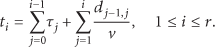
An $\mathcal{M}\mathcal{C}$ periodically charges along tour $R_i$ with charging period $T_i$ ( $\mathrm{1}\le i\le z$ ). As will be proved in Section 4, $T_i$ of tour $R_i$ ranges in a feasible region $[T_i^l,T_i^u]$ . Assume that $T_i$ is rational. Within each charging period $T_i$ , the total time an $\mathcal{M}\mathcal{C}$ spends in moving and charging states is called the working time of $R_i$ , denoted by $T_i^w$ ( $T_i^w\le T_i$ ). Consequently, we also use a tuple $(T_i,T_i^w)$ to substitute for $R_i$ . However, if the charging period of $R_i$ has not been determined, the tour can be denoted by a triple $(T_i^l,T_i^u,{\omega }_i)$ , where ${\omega }_i$ is a working time function dependent on $T_i$ . The three representations of $R_i$ will be used interchangeably in the rest of the paper, where no ambiguity occurs.

Suppose $z_k$ tours ${\mathbb{R}}_k=\{R_{\mathrm{1}},R_{\mathrm{2}},\dots ,R_{z_k}\}$ are assigned to $M_k$ ( $\mathrm{1}\le z_k\le z$ ); then we define the element period of $M_k$ , denoted by $G_k$ , as the greatest common divisor of charging periods of these $z_k$ tours. Define the conflict ratio of $M_k$ as

$$\begin{array}{cc}& {\delta }_k=\frac{{\sum }_{i=\mathrm{1}}^{z_k}{T}_i^w}{G_k},G_k=\text{GCD}\left(T_{\mathrm{1}},T_{\mathrm{2}},\dots ,T_{z_k}\right),\end{array}$$

(2)

where function $\text{GCD}(·)$ returns the greatest common divisor of the given numbers. Informally speaking, ${\delta }_k$ indicates the maximum work load of $M_k$ within any element period $G_k$ ; during $G_k$ , $M_k$ charges along $R_i\in {\mathbb{R}}_k$ for at most once. We will prove that if ${\delta }_i$ of $M_i$ is no more than 1, a valid charging schedule of charging along these k tours can be easily constructed. For instance, in Figure 2, $R_{\mathrm{1}}=(\mathrm{7.5,1})$ and $R_{\mathrm{2}}=(\mathrm{5,1.5})$ can be assigned to one $\mathcal{M}\mathcal{C}$ . Because the element period of the $\mathcal{M}\mathcal{C}$ is $G=\text{GCD}(T_{\mathrm{1}},T_{\mathrm{2}})=\text{GCD}(\mathrm{7.5,5})=\mathrm{2.5}$ , the conflict ratio of the $\mathcal{M}\mathcal{C}$ is $\delta =\left(T_{\mathrm{1}}^w+T_{\mathrm{2}}^w\right)/G=\left(\mathrm{1}+\mathrm{1.5}\right)/\mathrm{2.5}=\mathrm{1}$ .

Figure 2

Assigning $R_{\mathrm{1}}$ an $R_{\mathrm{2}}$ to one $\mathcal{M}\mathcal{C}$ .

Then the problem addressed in this paper can be formulated as follows.

Minimum Mobile Chargers Problem (MMCP). Given n sensor nodes $\mathbb{N}=\{N_i\hspace{0.17em}\hspace{0.17em}(p_i,E_S)\hspace{0.17em}|\hspace{0.17em}1\le i\le n\}$ and their positions in a WRSN, decide the minimum size m of $\mathbb{M}=\{M_i\hspace{0.17em}\hspace{0.17em}(q_c,q_m,v,E_M)\hspace{0.17em}|\hspace{0.17em}1\le i\le m\}$ to accomplish the charging mission.

When obtaining the minimum number of $\mathcal{M}\mathcal{C}$ s, a valid charging schedule should be constructed at the same time. To this end, the GCHA scheme constructs a set of schedulable tours that 1-covers the WRSN. Then it assigns the tours to minimum number of $\mathcal{M}\mathcal{C}$ s. Each $\mathcal{M}\mathcal{C}$ applies the GCS to charge along its assigned tours. The notations appearing in this paper are listed in Notations for readers’ convenience.

4. The Tour Construction Problem

Tours in $\mathbb{R}$ should fully cover the WRSN; we consider a scenario that these tours form an exact 1-cover of the WRSN. In other words, intersection of any two tours is empty, and any sensor node can appear in any tour for at most once:

$$\begin{array}{cc}& R_i\cap R_j=⌀,R_i,R_j\in \mathbb{R},\\ N_i\ne N_j,N_i,N_j\in R_k,\hspace{0.17em}\hspace{0.17em}{R}_k\in \mathbb{R}.\end{array}$$

(3)

Then we propose and address the following problem.

Tour Construction Problem (TCP). Given n sensor nodes $\mathbb{N}=\{N_i\hspace{0.17em}\hspace{0.17em}(p_i,E_S)\hspace{0.17em}|\hspace{0.17em}1\le i\le n\}$ and their positions in a WRSN, construct minimum number of tours $\mathbb{R}$ , schedulable to $\mathcal{M}\mathcal{C}$ s $(q_c,q_m,v,E_M)$ , to exactly 1-cover the WRSN.

The decision form of the TCP is NP-hard, since TCP contains DVRP as a subproblem [8]. A simple transformation is to let $n·E_S\to \mathrm{0}$ ; then the TCP can be reduced to a DVRP with distance constraint $E_M/q_m$ . To address the TCP, we firstly propose a sufficient condition for an $\mathcal{M}\mathcal{C}$ to be able to charge along a tour. The condition is derived from a Greedy Charging Scheme (GCS). Then, based on the decision condition, we greedily split the shortest Hamilton cycle through $\mathcal{S}$ and $\mathbb{N}$ into minimum number of schedulable subtours. The procedure is elaborated below.

4.1. The Greedy Charging Scheme

When charging along a tour $R=〈N_{\mathrm{0}},N_{\mathrm{1}},\dots ,N_r〉$ ( $\mathrm{1}\le r\le n$ ), an $M\in \mathbb{M}$ applies the GCS as follows. In each period, M starts from $N_{\mathrm{0}}$ , sequentially fully charges each sensor node, then returns to $N_{\mathrm{0}}$ , quickly renews its battery, and rests until next period. Denote that M arrives at $N_i$ at time $t_i$ and charges $N_i$ for time ${\tau }_i$ ; then we have

$$\begin{array}{cc}& t_i={\displaystyle \sum }_{j=\mathrm{0}}^{i-\mathrm{1}}{\tau }_j+{\displaystyle \sum }_{j=\mathrm{1}}^i\frac{d_{j-\mathrm{1},j}}{v},\mathrm{1}\le i\le r.\end{array}$$

(4)

In (4), $d_{i,j}$ is the distance between $N_i$ and $N_j$ and ${\tau }_{\mathrm{0}}\ge \mathrm{0}$ is the duration that M rests at $\mathcal{S}$ , and let $t_{\mathrm{0}}=\mathrm{0}$ to simplify the presentation. Then M can periodically charge along R with charging period

$$\begin{array}{cc}& T={\displaystyle \sum }_{j=\mathrm{0}}^r{\tau }_j+\frac{D}{v},\end{array}$$

(5)

where $D={\sum }_{j=\mathrm{1}}^r{d}_{j-\mathrm{1},j}+d_{r,\mathrm{0}}$ is the total traveling distance of the tour. Then, within each charging period, the energy consumed by $N_i$ can be fully replenished by M; that is,

$$\begin{array}{cc}& {\tau }_i·q_c·\eta =p_i·T,\mathrm{1}\le i\le r.\end{array}$$

(6)

To ensure the sensor nodes are working continuously, their energy levels should never fall below 0 during T; that is,

$$\begin{array}{cc}& E_S-p_i·\left(T-{\tau }_i\right)\ge \mathrm{0},\mathrm{1}\le i\le r.\end{array}$$

(7)

Meanwhile, the total energy of M should be enough to conduct charging; that is,

$$\begin{array}{cc}& D·q_m+\hspace{0.17em}{\displaystyle \sum }_{j=\mathrm{1}}^r·q_c·{\tau }_j\le E_M.\end{array}$$

(8)

Therefore, M can charge along tour R applying the GCS if and only if it satisfies (4)–(8).

4.2. Deriving the Decision Condition

According to the formulation of the GCS, we can derive an efficient decision condition to decide whether a tour is schedulable. The decision condition, named Tour Schedulable (TS) condition, can be used to construct schedulable tours to exactly 1-cover the WRSN.

Equation (6) can be rewritten as

$$\begin{array}{cc}& {\tau }_i=\frac{p_i·T}{q_c·\eta },\mathrm{1}\le i\le r.\end{array}$$

(9)

Thus the charging duration of each sensor node is dependent on its charging period T. In fact, T determines the charging schedule of M applying the GCS, according to (4) and (9). Furthermore, T also determines the working time of R:

$$\begin{array}{cc}& T^w={\displaystyle \sum }_{i=\mathrm{1}}^n{\tau }_i+\frac{D}{v}=\frac{p_{\text{sum}}}{q_c·\eta }·T+\frac{D}{v}.\end{array}$$

(10)

Obviously, $T^w$ increases as T increases; however, $T^w/T$ decreases as T increases. Literature [12] presented that $T^w/T$ indicates the total energy consumption of M in charging along R; thus it should be minimized. Plugging (9) into (5) we have

$$\begin{array}{cc}& T={\tau }_{\mathrm{0}}+\frac{{\sum }_{i=\mathrm{1}}^r{p}_i·T}{q_c·\eta }+\frac{D}{v}\ge \frac{{\sum }_{i=\mathrm{1}}^r{p}_i·T}{q_c·\eta }+\frac{D}{v},\end{array}$$

(11)

or, equivalently,

$$\begin{array}{cc}& T\ge \frac{D·q_c·\eta }{v·\left(q_c·\eta -p_{\text{sum}}\right)},p_{\text{sum}}={\displaystyle \sum }_{i=\mathrm{1}}^r{p}_i.\end{array}$$

(12)

Let $T^l=\left(D·q_c·\eta \right)/\left(v·(q_c·\eta -p_{\text{sum}})\right)$ ; then feasible charging period of tour R cannot be less than $T^l$ ; otherwise M does not have enough time to charge all the sensor nodes in R. Note that, to make (12) work, a necessary condition should be met: $q_c·\eta >p_{\text{sum}}$ .

Plugging (9) into (7) we have

$$\begin{array}{cc}& E_S\ge \frac{p_i·\left(q_c·\eta -p_i\right)}{q_c·\eta }·T,\mathrm{1}\le i\le r.\end{array}$$

(13)

Since $q_c·\eta >p_{\text{sum}}>p_i$ , the inequality is equal to

$$\begin{array}{cc}& T\le \frac{E_s·q_c·\eta }{p_{\text{mx}}},p_{\text{mx}}=\underset{\mathrm{1}\le i\le r}{\text{max}}\hspace{0.17em}{p}_i·\left(q_c·\eta -p_i\right).\end{array}$$

(14)

Let $T^u=\left(E_s·q_c·\eta \right)/p_{\text{mx}}$ ; then feasible charging period of R cannot exceed $T^u$ , or some sensor node will run out of energy before it is charged. Combining (12) and (14) we have

$$\begin{array}{cc}& \frac{D·q_c·\eta }{v·\left(q_c·\eta -p_{\text{sum}}\right)}\le \frac{E_s·q_c·\eta }{p_{\text{mx}}}\end{array}$$

(15)

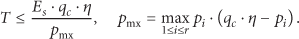
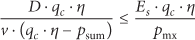
or, equivalently, $v\ge \left(D·p_{\text{mx}}\right)/\left(E_S·(q_c·\eta -p_{\text{sum}})\right)$ , which is also a necessary condition for R to have feasible charging period. Plugging (9) into (8) we have

$$\begin{array}{cc}& E_M\ge D·q_m+\frac{p_{\text{sum}}}{\eta }·T.\end{array}$$

(16)

Formula (16) shows the minimum energy required for an $\mathcal{M}\mathcal{C}$ to charge along R with charging period T. Let $T=T^u$ ; we have $E_M\ge \left(E_S·q_c·p_{\text{sum}}\right)/p_{\text{mx}}+D·q_m$ . By now, we have derived a sufficient condition for M to charge along R.

TS Condition. An $\mathcal{M}\mathcal{C}$ applying the GCS can charge along tour $R=〈N_0,N_1,\dots ,N_r〉$ if (a) $q_c·\eta >p_{\text{sum}}$ ; (b) $v\ge \left(D·p_{\text{mx}}\right)/\left(E_S·(q_c·\eta -p_{\text{sum}})\right)$ ; (c) $E_M\ge D·q_m+\left(p_{\text{sum}}·E_S·q_c\right)/p_{\text{mx}}$ .

Note that in deriving the TS condition, we let $T=T^u$ to decide the minimum energy requirement of an $\mathcal{M}\mathcal{C}$ . One can set other feasible T to derive a new sufficient condition, or say anchoring other values of T for short. In the next section, however, we will show that anchoring $T=T^u$ can minimize the total energy consumption of the $\mathcal{M}\mathcal{C}$ s, as well as the conflict ratio it generated.

Although the TS condition is not necessary for a tour to be schedulable [26], $q_c·\eta >p_{\text{sum}}$ is a hard condition for any $\mathcal{M}\mathcal{C}$ to be able to charge along any tour. Furthermore, if the total charging power of $\mathbb{M}$ is not larger than the total energy consumption rate of $\mathbb{N}$ in the WRSN, the charging mission cannot be accomplished. Therefore, we obtain a lower bound of the number of $\mathcal{M}\mathcal{C}$ s needed to solve the MMCP.

Lower Bound $m^{\ast }$ . Given n sensor nodes $\mathbb{N}=\{N_i\hspace{0.17em}\hspace{0.17em}(p_i,E_S)\hspace{0.17em}|\hspace{0.17em}1\le i\le n\}$ and their positions in a WRSN, the minimum number of $\mathcal{M}\mathcal{C}$ s $(q_c,q_m,v,E_M)$ needed to accomplish the charging mission is not less than $m^{\ast }=⌈{\sum }_{i=1}^n{p}_i/\left(q_c·\eta \right)⌉$ .

The lower bound $m^{\ast }$ is not tight, since it only considers the influence of charging. Obviously, an $\mathcal{M}\mathcal{C}$ also spends time and energy on moving. Therefore, a more rigorous lower bound should be not less than $m^{\ast }$ . However, determining $m^{\ast }$ is very simple and efficient; thus we use $m^{\ast }$ for performance evaluation in Section 4.

Based on the TS condition, we propose Algorithm 1 to decide whether a tour can be assigned to an $\mathcal{M}\mathcal{C}$ (lines (1)–(7)). If the tour is schedulable, then Algorithm 1 returns the feasible region of its charging period (lines (8)-(9)) and the corresponding working time function (line (10)).

Algorithm 1: Decide whether an $$\mathcal{M}\mathcal{C}$$ can charge along R.

Require:

   R = $$〈N_{\mathrm{0}},N_{\mathrm{1}},\dots ,N_r〉$$ ,   $$E_S$$ , $$q_m$$ , $$q_c$$ , v, $$E_M$$ , η;

Ensure:

   Schedulability of R; $$(T^l$$ , $$T^u$$ , $$\omega )$$ .

( $$\mathit{1}$$ ) calculate path length D of R;

( $$\mathit{2}$$ ) inquire energy consumption rates $$\{p_i\}$$ of the sensor nodes in R;

( $$\mathit{3}$$ ) $$p_{\text{sum}}={\displaystyle \sum }_{i=\mathit{1}}^r{p}_i$$ ;

( $$\mathit{4}$$ ) $$p_{\mathrm{m}\mathrm{x}}=\underset{\mathrm{1}\le i\le r}{\text{max}}{p}_i\cdot (q_c\cdot \eta -p_i)$$ ;

( $$\mathit{5}$$ ) if the conditions in Proposition 2 are not satisfied then

( $$\mathit{6}$$ )  return unschedulable;

( $$\mathit{7}$$ ) end if

( $$\mathit{8}$$ ) $$T^l=\frac{D\cdot q_c\cdot \eta }{v\cdot (q_c\cdot \eta -p_{\mathrm{s}\mathrm{u}\mathrm{m}})}$$ ;

( $$\mathit{9}$$ ) $$T^u=\frac{E_s\cdot q_c\cdot \eta }{p_{\mathrm{m}\mathrm{x}}}$$ ;

( $$\mathit{10}$$ ) $$\omega (T)=\frac{p_{\mathrm{s}\mathrm{u}\mathrm{m}}}{q_c\cdot \eta }\cdot T+\frac{D}{v}$$ ;

( $$\mathit{11}$$ ) return schedulable;

4.3. Obtaining Schedulable Subtours

Since TCP is NP-hard, based on the TS condition, we propose a greedy solution, as shown in Algorithm 2. First, we construct a Hamilton tour H through $\mathcal{S}$ and $\mathbb{N}$ by applying LKH algorithm [27] (lines (2)-(3)). Then we replace edges $e_{i,i+\mathrm{1}}$ and $e_{j,j+\mathrm{1}}$ by $e_{\mathrm{0},i+\mathrm{1}}$ and $e_{j,\mathrm{0}}$ (lines (5), (7)) and decide whether an $\mathcal{M}\mathcal{C}$ can charge along tour $〈N_{\mathrm{0}},N_{i+\mathrm{1}},\dots ,N_j〉$ using Algorithm 1 (line (8)). A subtour is constructed if no more sensor nodes can be inserted (lines (9)–(13)). Repeat the procedure until all sensor nodes are covered (line (4)). In this way, we greedily split H into z schedulable subtours. Figure 3 shows a demonstration of Algorithm 2, in which two schedulable tours are constructed to cover the 5-node WRSN. Computation complexity of verifying Proposition 2 is $O(r)$ . If variables such as $p_{\text{sum}}$ and $p_{\text{mx}}$ can be saved in the algorithm, the complexity of updating these information is $O(1)$ . Then lines (3)–(15) can be executed with complexity $O(n)$ . Therefore, the computation complexity of Algorithm 2 is dependent on that of LKH, which is $O(n^{2.2})$ [27]. Note that H is not necessarily the shortest Hamilton cycle through the WRSN. In fact, it only provides a sequence of sensor nodes. Therefore, H can be any permutation of the sensor nodes. For instance, H can be obtained by sorting the sensor nodes in ascending order of their energy consumption rates. In this way, sensor nodes in each constructed subtour have similar energy consumption rates and greatly relief the load imbalance phenomenon [12], which causes great waste in periodic charging schemes. From this viewpoint, a periodic charging scheme using multiple $\mathcal{M}\mathcal{C}$ s is similar to an on-demand charging scheme using one $\mathcal{M}\mathcal{C}$ . Nevertheless, total distance of each subtour should be minimized [10]. Therefore, it is a compromise that we made in designing Algorithm 2.

Algorithm 2: Construct a Hamilton tour H through $$\mathcal{S}$$ and $$\mathbb{N}$$ ; split H into z schedulable subtours.

Require:

    $$\mathbb{N}=\{N_i\hspace{0.17em}|\hspace{0.17em}\mathit{1}\le i\le n\}$$ ;

Ensure:

    $$\mathbb{R}=\{R_i\hspace{0.17em}|\hspace{0.17em}\mathit{1}\le i\le z\}$$ ;

( $$\mathit{1}$$ ) $$z=\mathrm{1},\hspace{0.17em}\hspace{0.17em}i=\mathrm{1}$$ ;

( $$\mathit{2}$$ ) apply LKH on $$\mathcal{S}\cup \mathbb{N}$$ to obtain H;

( $$\mathit{3}$$ ) renumber sensor nodes in H as $$N_{\mathrm{0}},N_{\mathrm{1}},\dots ,N_n$$ ( $$N_{\mathrm{0}}=\mathcal{S}$$ );

( $$\mathit{4}$$ )    while   $$i\le n$$   do

( $$\mathit{5}$$ )     push $$N_{\mathrm{0}}$$ into $$R_z$$ ;

( $$\mathit{6}$$ )     for   $$j=i$$   to  n  do

( $$\mathit{7}$$ )      push $$N_j$$ into $$R_z$$ ;

( $$\mathit{8}$$ )      apply Algorithm 1 to decide the schedulability of $$R_z$$ ;

( $$\mathit{9}$$ )      if   $$R_z$$ is unschedulable  then

( $$\mathit{10}$$ )      pop $$N_j$$ from $$R_z$$ ;

( $$\mathit{11}$$ )       $$i=j,\hspace{0.17em}\hspace{0.17em}z=z+\mathrm{1}$$ ;

( $$\mathit{12}$$ )      break;

( $$\mathit{13}$$ )    end if

( $$\mathit{14}$$ )   end for

( $$\mathit{15}$$ ) end while

Figure 3

Demonstration of the tour construction algorithm.

5. The Tour Assignment Problem

After obtaining schedulable subtours that 1-cover all the sensor nodes, we further assign these subtours to minimum number of $\mathcal{M}\mathcal{C}$ s. To this end, we firstly formulate the Tour Assignment Problem (TAP) and prove its NP-hardness. Then we propose a heuristic algorithm to solve the problem. Every tour discussed in this section is schedulable.

5.1. The Tour Assignment Problem

According to the abovementioned analysis, feasible charging period $T_i$ of tour $R_i$ ranges from $T_i^l$ to $T_i^u$ , which also decides the working time $T_i^w$ of $R_i$ in each period: $T_i^w={\omega }_i(T_i)=\left(p_{\text{sum}}^i/\left(q_c·\eta \right)\right)·T_i+D_i/v$ . Then the assignment problem can be formulated as follows.

Tour Assignment Problem (TAP). Given z tours $\mathbb{R}=\{R_i=(T_i^l,T_i^u,{\omega }_i)\hspace{0.17em}|\hspace{0.17em}1\le i\le z\}$ and enough $\mathcal{M}\mathcal{C}$ s $(q_c,q_m,v,E_M)$ , assign tours $\mathbb{R}$ to minimum number of $\mathcal{M}\mathcal{C}$ s.

To prove the NP-hardness of the TAP, we firstly consider r tours with equal charging period T and investigate the sufficient and necessary condition of assigning these r tours to one $\mathcal{M}\mathcal{C}$ .

Proposition 1.

Given r tours $\{R_i=(T,T_i^w)\hspace{0.17em}|\hspace{0.17em}\mathrm{1}\le i\le r\}$ , they can be assigned to one $\mathcal{M}\mathcal{C}$ if and only if ${\sum }_{i=\mathrm{1}}^r{T}_i^w\le T$ .

Proof.

Suppose these k tours can be assigned to the same $\mathcal{M}\mathcal{C}$ ; then ${\sum }_{i=\mathrm{1}}^r{T}_i^w\le T$ . Otherwise the $\mathcal{M}\mathcal{C}$ cannot finish charging along all tours within one charging period T, causing conflicts in the next period.

On the other hand, if ${\sum }_{i=\mathrm{1}}^r{T}_i^w\le T$ , one can construct a valid schedule as follows. The $\mathcal{M}\mathcal{C}$ charges sensor nodes in $R_i$ during time $[k·T+{\sum }_{j=\mathrm{1}}^{i-\mathrm{1}}{T}_j^w,k·T+{\sum }_{j=\mathrm{1}}^i{T}_j^w]$ ( $k=\mathrm{0,1},\mathrm{2},\dots$ ). Since ${\sum }_{i=\mathrm{1}}^r{T}_i^w\le T$ , this schedule is valid.

Therefore, the proposition follows.

Based on Proposition 1, we reduce the TAP to a set-partition problem and consequently prove that the decision form of the problem is NP-hard.

Proposition 2.

Deciding whether z tours can be assigned to m  $\mathcal{M}\mathcal{C}$ s is NP-hard.

Proof.

Consider z tours $\{R_i=(T,T_i^w)\hspace{0.17em}|\hspace{0.17em}\mathrm{1}\le i\le z\}$ , and suppose ${\sum }_{i=\mathrm{1}}^z{T}_i^w=\mathrm{2}T$ . Let $m=\mathrm{2}$ ; then the decision problem can be reformulated as whether $\{R_i\}$ can be assigned to 2 $\mathcal{M}\mathcal{C}$ s.

We now construct a set-partition problem as follows. Given z numbers $\{a_{\mathrm{1}},a_{\mathrm{2}},\dots ,a_z\}$ , in which $a_i=T_i^w/T$ ( $\mathrm{1}\le i\le z$ ), then, according to Proposition 1, the above question is equivalent to whether the z numbers can be evenly partitioned into two sets. Since the set-partition problem is NP-hard, the original problem is also NP-hard.

5.2. The Heuristic Solution

We propose a heuristic method to decide (a) the charging period of each tour and (b) whether a set of tours with fixed charging periods can be assigned to one $\mathcal{M}\mathcal{C}$ .

We firstly generalize the assumption in Proposition 1 and assume that tours have different charging periods. Then we derive a necessary condition for these tours to be assigned to the same $\mathcal{M}\mathcal{C}$ . Suppose that the periods of all tours are rational numbers and their greatest common divisor is G (G can be a decimal); then we have the following proposition.

Proposition 3.

Given k set of tours: $\{R_i^j=(a_j·G,T_i^j)\hspace{0.17em}|\hspace{0.17em}\mathrm{1}\le i\le r_j,\hspace{0.17em}\hspace{0.17em}\mathrm{1}\le j\le k\}$ , where $R_i^j$ is the ith tour of the jth set and $\{a_j\}$ are coprime integers, these tours can be assigned to one $\mathcal{M}\mathcal{C}$ only if ${\sum }_{j=\mathrm{1}}^k\left({\sum }_{i=\mathrm{1}}^{r_j}{T}_i^j/a_j\right)\le G$ .

Proof.

Suppose these tours can be assigned to one $\mathcal{M}\mathcal{C}$ , while ${\sum }_{j=\mathrm{1}}^k\left({\sum }_{i=\mathrm{1}}^{r_j}{T}_i^j/a_j\right)>G$ . Denote the least common multiple of $a_{\mathrm{1}},a_{\mathrm{2}},\dots ,a_k$ by P. Multiplying both sides of the inequality by P, we have

$$\begin{array}{cc}& \frac{P}{a_{\mathrm{1}}}·{\displaystyle \sum }_{i=\mathrm{1}}^{r_{\mathrm{1}}}{T}_i^{\mathrm{1}}+\frac{P}{a_{\mathrm{2}}}·{\displaystyle \sum }_{i=\mathrm{1}}^{r_{\mathrm{2}}}{T}_i^{\mathrm{2}}+\cdots +\frac{P}{a_k}·{\displaystyle \sum }_{i=\mathrm{1}}^{r_k}{T}_i^k>G·P,\end{array}$$

(17)

where $P/a_j$ means how many times does the $\mathcal{M}\mathcal{C}$ charge along tours $\{R_i^j\}$ during $G·P$ and ${\sum }_{i=\mathrm{1}}^{r_j}{T}_i^j$ is the total working time of the jth set of tours within each charging period $a_j·G$ . It means that the total working time of all the tours during $G·P$ is larger than $G·P$ , which is a contradiction.

Therefore, the proposition follows.

Unfortunately, the condition is not sufficient, because it requires that the jth set of tours can be evenly partitioned into $a_j$ parts, such that the total working time of tours in each part is the same. Otherwise these tours are not surely schedulable. For example, tours $\{\mathrm{2}T,\mathrm{2}T/\mathrm{3}\}$ , $\{\mathrm{2}T,T/\mathrm{3}\}$ , and $\{T,T/\mathrm{2}\}$ cannot be charged by one $\mathcal{M}\mathcal{C}$ even if they satisfy Proposition 3. Besides, deciding whether the jth set of tours can be evenly partitioned into $a_j$ parts is NP-hard, since it can be easily reduced to a set-partition problem. Therefore, we propose the following sufficient condition for efficiently deciding whether r tours can be assigned to one $\mathcal{M}\mathcal{C}$ .

Proposition 4.

Given r tours $\{R_i=(a_i·G,T_i^w)\hspace{0.17em}|\hspace{0.17em}\mathrm{1}\le i\le r\}$ , where $\{a_i\}$ are coprime integers, they can be assigned to one $\mathcal{M}\mathcal{C}$ if ${\sum }_{i=\mathrm{1}}^r{T}_i^w\le G$ .

Proof.

Consider r tours $\{R_i^{\prime }=(G,T_i^w)\hspace{0.17em}|\hspace{0.17em}\mathrm{1}\le i\le r\}$ ; if they can be assigned to one $\mathcal{M}\mathcal{C}$ , obviously $\{R_i\}$ can be assigned to the same $\mathcal{M}\mathcal{C}$ . Since ${\sum }_{i=\mathrm{1}}^r{T}_i^w\le G$ , according to Proposition 3, $\{R_i^{\prime }\}$ can be assigned to one $\mathcal{M}\mathcal{C}$ . Therefore, $\{R_i\}$ can be assigned to one $\mathcal{M}\mathcal{C}$ .

Note that Proposition 4 is not necessary. For instance, consider tour $R^A=(T,T/\mathrm{2})$ and r tours $\{R_i^B=(r·T,T/\mathrm{2})\hspace{0.17em}|\hspace{0.17em}r>\mathrm{1},\hspace{0.17em}\hspace{0.17em}\mathrm{1}\le i\le r\}$ . Since $\text{GCD}(T,r·T)=T$ , and the total working time of the $r+\mathrm{1}$ tours is $\left((r+\mathrm{1})/\mathrm{2}\right)·T>T$ , the condition in Proposition 4 is not met. However, one can still assign them to one $\mathcal{M}\mathcal{C}$ : let the $\mathcal{M}\mathcal{C}$ charge along tour $R^A$ during time $[j·T,(j+\mathrm{1}/\mathrm{2})·T]$ and charge along tour $R_i^B$ during time $[(j·r+i-\mathrm{1}/\mathrm{2})·T,(j·r+i)·T]$ , $j=\mathrm{0,1},\mathrm{2},\dots$ . It can be readily proved that the charging schedule is valid.

Proposition 4 inspires us to minimize the conflict ratio of each $\mathcal{M}\mathcal{C}$ : $\delta ={\sum }_{i=\mathrm{1}}^r\left(T_i^w/G\right)$ . If it is no more than 1, valid charging schedule can be readily constructed. Based on this idea, we propose the following heuristic rule to determine the charging period of each tour.

Proposition 5.

Suppose tours $R_{\mathrm{1}}=(T_{\mathrm{1}}^l,T_{\mathrm{1}}^u,{\omega }_{\mathrm{1}})$ and $R_{\mathrm{2}}=(T_{\mathrm{2}}^l,T_{\mathrm{2}}^u,{\omega }_{\mathrm{2}})$ are assigned to M, where $(k-\mathrm{1})·T_{\mathrm{1}}^u<T_{\mathrm{2}}^l\le k·T_{\mathrm{1}}^u\le T_{\mathrm{2}}^u$ ( $k\ge \mathrm{1}$ ); then the conflict ratio δ of M is minimized when $T_{\mathrm{1}}=T_{\mathrm{1}}^u$ and $T_{\mathrm{2}}=k·T_{\mathrm{1}}^u$ .

Proof.

For each tour $R_i$ , $\omega (T_i)=\left(p_{\text{sum}}^i/\left(q_c·\eta \right)\right)·T_i+D_i/v$ . To simplify the presentation, denote that $\omega (T_i)=a_i·T_i+b_i$ .

Consider δ when $T_{\mathrm{2}}$ varies within time interval $[i·T_{\mathrm{1}},(i+\mathrm{1})·T_{\mathrm{1}}]$ ( $i=\mathrm{1,2},\dots$ ):

$$\begin{array}{l}{\delta }_{\mathrm{1}}=a_{\mathrm{1}}+i·a_{\mathrm{2}}+\frac{b_{\mathrm{1}}+b_{\mathrm{2}}}{T_{\mathrm{1}}},T_{\mathrm{2}}=i·T_{\mathrm{1}},\\ {\delta }_{\mathrm{2}}=a_{\mathrm{1}}+\left(i+\mathrm{1}\right)·a_{\mathrm{2}}+\frac{b_{\mathrm{1}}+b_{\mathrm{2}}}{T_{\mathrm{1}}},T_{\mathrm{2}}=\left(i+\mathrm{1}\right)·T_{\mathrm{1}},\\ {\delta }_{\mathrm{3}}=\frac{a_{\mathrm{1}}·T_{\mathrm{1}}+a_{\mathrm{2}}·T_{\mathrm{2}}}{G}+\frac{b_{\mathrm{1}}+b_{\mathrm{2}}}{G},\\ i·T_{\mathrm{1}}<T_{\mathrm{2}}<\left(i+\mathrm{1}\right)·T_{\mathrm{1}},\end{array}$$

(18)

where $G=\text{GCD}(T_{\mathrm{1}},T_{\mathrm{2}})$ . When $i·T_{\mathrm{1}}<T_{\mathrm{2}}<(i+\mathrm{1})·T_{\mathrm{1}}$ , $G\le T_{\mathrm{1}}/\mathrm{2}$ , we hence have

$$\begin{array}{l}{\delta }_{\mathrm{3}}=\frac{a_{\mathrm{1}}·T_{\mathrm{1}}+a_{\mathrm{2}}·T_{\mathrm{2}}}{G}+\frac{b_{\mathrm{1}}+b_{\mathrm{2}}}{G}\\ \ge \mathrm{2}{a}_{\mathrm{1}}+\mathrm{2}i·a_{\mathrm{2}}+\frac{\mathrm{2}\left(b_{\mathrm{1}}+b_{\mathrm{2}}\right)}{T_{\mathrm{1}}}\\ >a_{\mathrm{1}}+\left(i+\mathrm{1}\right)·a_{\mathrm{2}}+\frac{b_{\mathrm{1}}+b_{\mathrm{2}}}{T_{\mathrm{1}}}={\delta }_{\mathrm{2}}.\end{array}$$

(19)

In other words, ${\delta }_{\mathrm{1}}<{\delta }_{\mathrm{2}}<{\delta }_{\mathrm{3}}$ . Therefore, in this scenario, δ is minimized when $T_{\mathrm{2}}=i·T_{\mathrm{1}}$ . Then $\delta =a_{\mathrm{1}}+i·a_{\mathrm{2}}+\left(b_{\mathrm{1}}+b_{\mathrm{2}}\right)/T_{\mathrm{1}}$ .

On the other hand, δ decreases as $T_{\mathrm{1}}$ increases. To minimize δ, we have $T_{\mathrm{1}}=T_{\mathrm{1}}^u$ . Since $(k-\mathrm{1})·T_{\mathrm{1}}^u<T_{\mathrm{2}}^l\le k·T_{\mathrm{1}}^u\le T_{\mathrm{2}}^u$ , we have $i=k$ ; that is, $T_{\mathrm{2}}=k·T_{\mathrm{1}}^u$ .

In summary, δ is minimized when $T_{\mathrm{1}}=T_{\mathrm{1}}^u$ and $T_{\mathrm{2}}=k·T_{\mathrm{1}}^u$ ; then the proposition follows.

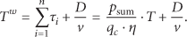
In fact, Proposition 5 requires the element period G of M to be maximized. This is an important reason that we anchor $T=T^u$ when deriving the TS condition. Note that one can set $T=T^{\prime }$ ( $T^l\le T^{\prime }<T^u$ ) in deriving the TS condition. In this way, the number of subtours may be reduced in Algorithm 2. Nevertheless, these tours are harder to be assigned to one $\mathcal{M}\mathcal{C}$ according to Proposition 5. More importantly, anchoring smaller value of T will increase the total working time ratio (denoted by ${\Phi }_w$ ) of the $\mathcal{M}\mathcal{C}$ s:

$$\begin{array}{cc}& {\Phi }_w={\displaystyle \sum }_{i=\mathrm{1}}^m{\displaystyle \sum }_{j=\mathrm{1}}^{z_i}\frac{T_j^w}{T_j}={\displaystyle \sum }_{i=\mathrm{1}}^z\frac{T_i^w}{T_i}.\end{array}$$

(20)

We have proved in [12] that the working time ratio of an $\mathcal{M}\mathcal{C}$ indicates the total energy consumption of the $\mathcal{M}\mathcal{C}$ in conducting charging. Therefore, ${\Phi }_w$ indicates the total energy consumption of all the $\mathcal{M}\mathcal{C}$ s. Based on the above two reasons, we anchor $T=T^u$ in deriving the TS condition. Comparisons of anchoring different values of T are made through simulations.

Based on the heuristic rules formulated in Propositions 4 and 5, we propose Algorithm 3 to greedily assign maximum number of tours to each $\mathcal{M}\mathcal{C}$ . First, the tours obtained by Algorithm 2 are sorted by $T^u$ in ascending order (line (2)). Then, for each $\mathcal{M}\mathcal{C}$ , sequentially consider if tour $R_i$ can be assigned to it (lines (3)–(18)). According to Proposition 5, the element period $G_k$ of $M_k$ is set to $T_i^u$ of its first assigned tour $R_i$ (line (7)). For any subsequent tour $R_j$ , it is assigned to $M_k$ (lines (6), (13)) if

• (a)

$R_j$ has not been assigned to any $\mathcal{M}\mathcal{C}$ (lines (4), (9)),

(b)

feasible period of $R_j$ contains a multiple of $G_k$ (lines (10)-(11)),

(c)

after assigning, the conflict ratio ${\delta }_k$ of $M_k$ is still no more than 1 (line (11)).

Then charging period $T_j$ of $R_j$ is determined according to Proposition 5 (lines (7), (12)). It can be readily proved that the worst case computation complexity of Algorithm 3 is $O(z^2)$ , where z is the number of tours.

Algorithm 3: Sort tours $$\mathbb{R}$$ by $$T^u$$ ; greedily assign the tours to minimum $$\mathcal{M}\mathcal{C}$$ s based on Propositions 4 and 5.

Require:

       $$\mathbb{R}=\{R_i\hspace{0.17em}|\hspace{0.17em}\mathit{1}\le i\le z\}$$ ;

Ensure:

       $$\mathbb{M}=\{M_i\hspace{0.17em}|\hspace{0.17em}\mathit{1}\le i\le m\}$$ , tour assignment of each $$\mathcal{M}\mathcal{C}$$ ;

( $$\mathit{1}$$ )     $$m=\mathrm{0}$$ ;

( $$\mathit{2}$$ )    sort $$\{R_i\}$$ by $$T_i^u$$ in ascending order;

( $$\mathit{3}$$ )    for   $$i=\mathrm{1}$$   to  z  do

( $$\mathit{4}$$ )       if   $$R_i$$ has not been assigned  then

( $$\mathit{5}$$ )         $$m+=\mathrm{1}$$ ;

( $$\mathit{6}$$ )        assign $$R_i$$ to $$M_m$$ ;

( $$\mathit{7}$$ )         $$G_m=T_i=T_i^u$$ ,   $${\delta }_m=\frac{{\omega }_i\left(T_i\right)}{G_m}$$ ;

( $$\mathit{8}$$ )        for   $$j=i+\mathrm{1}$$   to  z  do

( $$\mathit{9}$$ )        if   $$R_j$$ has not been assigned  then

(10)        calculate the k described in Proposition 5;

( $$\mathit{11}$$ )        if  k exists  and   $${\delta }_m+({\omega }_j\left(k\cdot T_i^u\right)/G_m)\le \mathrm{1}$$   then

(12)          $$T_j=k\cdot T_i^u$$ ,   $${\delta }_m+=\frac{{\omega }_j\left(T_j\right)}{G_m}$$ ;

(13)         assign $$R_j$$ to $$M_m$$ ;

(14)        end if

(15)     end if

(16)     end for

(17)     end if

( $$\mathit{18}$$ ) end for

After tour assignment, each $\mathcal{M}\mathcal{C}$ applies the GCS to periodically charge along its assigned tours. Suppose $z_x$ tours ${\mathbb{R}}_x=\{R_i=(a_i·G_x,T_i^w)\}$ are assigned to $M_x$ ( $\mathrm{1}\le i\le z_x\le n$ , $\mathrm{1}\le x\le m$ ); then a valid charging schedule is that $M_x$ charges $R_i$ during time $[k·a_i·G_x+{\sum }_{j=\mathrm{1}}^{i-\mathrm{1}}{T}_j^w,k·a_i·G_x+{\sum }_{j=\mathrm{1}}^i{T}_j^w]$ ( $k=\mathrm{0,1},\mathrm{2},\dots$ ) and rests at $\mathcal{S}$ at other times. The details of the charging schedule are shown in Algorithm 4. However, when $M_x$ charges $R_i$ for the first time, since the sensor nodes are initially fully charged, the actual working time of tour $R_i$ is less than $T_i^w$ . This may influence subsequent periods. To address this issue, one can make $M_x$ stay at sensor node $N_j$ in $R_i$ for time $\left(p_j·T_i\right)/\left(q_c·\eta \right)$ and leave with $N_j$ fully charged. In this way, the actual working time of $R_i$ is $T_i^w$ afterwards.

Algorithm 4: Construct a valid charging schedule of $$M_k$$ along its assigned tours $${\mathbb{R}}_k$$ .

Require:

       $${\mathbb{R}}_k=\{R_i\hspace{0.17em}|\hspace{0.17em}\mathrm{1}\le i\le z_k\}$$ ;

Ensure:

       $$\{(R_i,〈t_j^i〉,〈{\tau }_j^i〉)\hspace{0.17em}|\hspace{0.17em}\mathrm{1}\le i\le z_k,\mathrm{1}\le j\le r_i\}$$ ;

( $$\mathit{1}$$ )     $${\tau }_{\mathrm{0}}^{\mathrm{1}}=\mathrm{0}$$ ;

( $$\mathit{2}$$ )    for   $$i=\mathrm{2}$$   to   $$z_k$$   do

( $$\mathit{3}$$ )      $${\tau }_{\mathrm{0}}^i={\tau }_{\mathrm{0}}^{i-\mathrm{1}}+T_{i-\mathrm{1}}^w$$ ;

( $$\mathit{4}$$ )    end for

( $$\mathit{5}$$ )    for   $$i=\mathrm{1}$$   to   $$z_k$$   do

( $$\mathit{6}$$ )      $$t_{\mathrm{0}}^i=\mathrm{0}$$ ;

( $$\mathit{7}$$ )      $${\tau }_j^i=\frac{T_i\cdot p_j}{q_c\cdot \eta }$$ ,  $$\mathrm{1}\le j\le r_i$$ ;

( $$\mathit{8}$$ )      $$t_j^i=t_{j-\mathrm{1}}^i+{\tau }_{j-\mathrm{1}}^i+\frac{d_{j-\mathrm{1},j}}{v}$$ ,  $$\mathrm{0}\le j\le r_i$$ ;

( $$\mathit{9}$$ )    end for

( $$\mathit{10}$$ ) $$k=\mathrm{0}$$ ;

( $$\mathit{11}$$ ) while ++k  do

( $$\mathit{12}$$ )  set current time to 0;

( $$\mathit{13}$$ )  for   $$i=\mathrm{1}$$   to  z  do

( $$\mathit{14}$$ )   if   $$k\hspace{0.17em}\hspace{0.17em}\mathrm{\%}\hspace{0.17em}\hspace{0.17em}{a}_i=\mathrm{0}$$   then

( $$\mathit{15}$$ )     $$\mathcal{M}\mathcal{C}$$ leaves $$\mathcal{S}$$ to charge along tour $$R_i$$ at time $${\tau }_{\mathrm{0}}^i$$ ;

( $$\mathit{16}$$ )    for   $$j=\mathrm{1}$$   to   $$r_i$$   do

( $$\mathit{17}$$ )      $$\mathcal{M}\mathcal{C}$$ arrives $$N_j^i$$ at $$t_j^i$$ , and charges it for $${\tau }_i^i$$ ;

( $$\mathit{18}$$ )    end for

( $$\mathit{19}$$ )     $$\mathcal{M}\mathcal{C}$$ returns to $$\mathcal{S}$$ , end of charging along tour $$R_i$$ ;

( $$\mathit{20}$$ )   end if

( $$\mathit{21}$$ )  end for

( $$\mathit{22}$$ ) end while

5.3. The Complete Procedure of the GCHA Solution

To summarize, the complete procedure of the GCHA solution is presented as follows. First, apply Algorithm 2 to construct z schedulable tours to 1-cover the WRSN. During this step, Algorithm 1 is constantly called to decide whether a tour of sensor nodes can be timely charged by one $\mathcal{M}\mathcal{C}$ . Second, apply Algorithm 3 to decide the charging period of each tour, and assign these tours to $m\hspace{0.17em}\hspace{0.17em}\mathcal{M}\mathcal{C}$ s. Then the $\mathcal{M}\mathcal{C}$ s apply Algorithm 4 to conduct charging along their assigned tours. The computation complexity of the solution is dependent on Algorithm 2, which is $O(n^{2.2})$ .

6. Numerical Results

In this section, we evaluate the performance of the GCHA solution. To this end, WRSNs are randomly generated over a 1000 m × 1000 m square area. The sink node and service station are located at the center of the area. The sensor nodes generate data at a random rate within $[\mathrm{10,100}]$  kbps, and their communication radius is 200 m. The energy consumption model is adopted from [10], in which only energy consumption of sending and receiving data is considered. Particularly, energy consumption of receiving a bit of data is a constant, while energy consumption of sending a bit of data is additionally dependent on the transmitting distance. The routing scheme is the well known GPSR [28], which is well scalable and also based on location information. By default, we set $E_S=\mathrm{10}$  kJ, $q_m=\mathrm{5}$  J/m, $v=\mathrm{5}$  m/s, $E_M=\mathrm{40}$  kJ, and $\eta =\mathrm{1}$ , which are adopted from [10] or with reasonable estimation.

6.1. Demonstration of the GCHA Solution

To better demonstrate the procedures of the GCHA solution, we randomly generate a 100-node WRSN, as shown in Figure 4, and set $q_c=\mathrm{5}$  W. The $\mathcal{S}$ and sink node are located at the center of the WRSN. According to Algorithm 2, we firstly apply LKH algorithm to construct a Hamilton tour H through $\mathcal{S}$ and $\mathbb{N}$ , as shown in Figure 5. Then, based on the decision results returned by Algorithm 1, we greedily split H into 10 schedulable subtours, as shown in Figure 6. It can be found that the tours nearer to the sink cover fewer sensor nodes, because sensor nodes around the sink can be exhausted faster due to larger forwarding burden. Then we call Algorithm 3 to assign these tours to 4 $\mathcal{M}\mathcal{C}$ s, and each $\mathcal{M}\mathcal{C}$ applies Algorithm 4 to conduct charging along its assigned tours.

Figure 4

Routing of the 100-node WRSN.

Figure 5

Shortest Hamilton cycle of the 100-node WRSN.

Figure 6

Schedulable subtours to cover the 100-node WRSN.

Figure 7 depicts the energy consumption of each $\mathcal{M}\mathcal{C}$ when charging along each tour within one charging period, in which the lighter grey part of a bar indicates the energy consumption of charging, while the darker grey part of a bar indicates the energy consumption of moving. The figure shows that the energy consumed in charging along different tours varies greatly. This is because, in the assigning procedure, the GCHA scheme selects T of $R_{\mathrm{1}}~R_{\mathrm{6}}$ nearly the same as their $T^u$ , while it selects T of $R_{\mathrm{7}}~R_{\mathrm{10}}$ much smaller than their $T^u$ . In consequence, when charging along $R_{\mathrm{7}}~R_{\mathrm{10}}$ , the energy consumption of the $\mathcal{M}\mathcal{C}$ is much less than $E_M$ . In turn, these tours contribute less conflict ratio of the $\mathcal{M}\mathcal{C}$ , as shown in Figure 8, so that the $\mathcal{M}\mathcal{C}$ can charge along more tours. The ratio of the grey area in a bar is the conflict ratio of an $\mathcal{M}\mathcal{C}$ . It can be seen that $M_{\mathrm{4}}$ achieves a relatively low conflict ratio. This is caused by the greedy nature of our solution. Balanced energy consumption of $\mathcal{M}\mathcal{C}$ s, however, is not a concern of this paper.

Figure 7

Energy consumption when charging along each tour.

Figure 8

Conflict ratios of each $\mathcal{M}\mathcal{C}$ .

6.2. Performance Evaluation

We then compare the number of $\mathcal{M}\mathcal{C}$ s m obtained by our solution with the lower bound $m^{\ast }$ to evaluate the performance. Specifically, we evaluate the approximation ratio of our results over the lower bound: $\alpha =m/m^{\ast }$ .

6.2.1. Varying Charging Power of $\mathcal{M}\mathcal{C}$ s

The total energy consumption rate of the WRSN shown in Figure 4 is $p_{\text{sum}}=\mathrm{15.24}$  W, and the corresponding $m^{\ast }=⌈\mathrm{15.24}/\mathrm{5}⌉=\mathrm{4}$ . Therefore, we actually give an optimum solution in the demonstration, regarding number of $\mathcal{M}\mathcal{C}$ s used. We further range charging power of the $\mathcal{M}\mathcal{C}$ s from 3 W to 9 W, and the comparison between m and $m^{\ast }$ is shown in Figure 9, where z is the number of subtours. It is clear that, in most cases, our method achieves optimum solutions of the MMCP. However, when $q_c=\mathrm{4}$  W and $q_c=\mathrm{8}$  W, our results are one more than $m^{\ast }$ . The reason will be explained later.

Figure 9

Results under different charging powers.

6.2.2. Varying Anchored Charging Period

We have explained the reason to anchor $T=T^u$ in deriving the TS condition. To verify its effectiveness, we anchor $T=\{T^l,((T^l+T^u))/\mathrm{4},((T^l+T^u))/\mathrm{2},(\mathrm{3}(T^l+T^u))/\mathrm{4},T^u\}$ and compare the performance of these schemes. We randomly generate 10 200-node WRSNs to test each anchored value of T; the results are shown in Figure 10. The blue stars show the averaged results achieved by the GCHA scheme; the red dots show the mean values of total working time ratios of the $\mathcal{M}\mathcal{C}$ s. It can be seen that m increases first and then decreases as T increases; m is minimum when $T=T^u$ . This is because when T is smaller, each obtained subtour can cover a larger number of sensor nodes; thus the number of tours is smaller; when T is larger, each obtained subtour contributed less conflict ratio of its $\mathcal{M}\mathcal{C}$ ; thus more tours can be assigned to the same $\mathcal{M}\mathcal{C}$ . Consequently when anchoring intermediate values of T, the number of obtained tours is relatively large, and these tours are hard to be assigned to the same $\mathcal{M}\mathcal{C}$ , leading to larger results of m. As for ${\Phi }_w$ , it monotonically increases as T increases. According to (10), $T^w/T$ of each tour decreases as T increases. Furthermore, as T increases, the influence of the decrease in $T^w/T$ is larger than that of the increase in tour numbers. Therefore, anchoring a larger value of T can reduce the total energy consumption of $\mathcal{M}\mathcal{C}$ s.

Figure 10

Results of anchoring different charging periods.

In conclusion, the results validate the effectiveness of anchoring $T=T^u$ in deriving the TS condition.

6.2.3. Varying Network Size

We compare the GCHA scheme with the NMV scheme proposed in [24]. NMV is an on-demand charging scheme. In [24], when the residual lifetime of a sensor node falls in the predefined critical lifetime interval, the sensor node will send an energy-recharging request to $\mathcal{S}$ for its energy replenishment. Once $\mathcal{S}$ receives the requests from sensor nodes, it performs the NMV scheme to dispatch a number of $\mathcal{M}\mathcal{C}$ s to charge the requested sensor nodes. To use minimum number of $\mathcal{M}\mathcal{C}$ s to meet the charging demand, the NMV scheme firstly constructs a minimum-cost spanning tree of the network. Then it decomposes the tree into minimum number of subtrees based on energy constraints of each $\mathcal{M}\mathcal{C}$ ; each of the subtrees can be assigned to one $\mathcal{M}\mathcal{C}$ . Then it derives closed charging tours from the subtrees, and the number of the tours equals the number of $\mathcal{M}\mathcal{C}$ s required. Since the NMV scheme is designed for low-power WRSNs, we let the sensor nodes generate data at a random rate within $[\mathrm{5,30}]$  kbps and range n from 100 to 500. With each size of n, we randomly generate 10 WRSNs for evaluation. The results are shown in Figure 11 and Table 1, in which $m^{\prime }$ is the results achieved by the NMV scheme.

Table 1

Approximation ratios of varying network size.

$$n=\mathrm{100}$$	$$m^{\ast }$$	1	1	1	1	1	2	2	2	2	2	$$\alpha =\mathrm{1.067}$$
	m	1	1	1	2	2	2	2	2	2	2
	$$p_{\mathrm{s}\mathrm{u}\mathrm{m}}$$	4.445	4.507	4.617	4.817	4.888	5.055	5.233	5.311	5.340	5.532
	$$q_c\cdot \eta \cdot m^{\ast }$$	5	5	5	5	5	10	10	10	10	10
$$n=\mathrm{200}$$	$$m^{\ast }$$	2	2	2	3	3	3	3	3	3	3	$$\alpha =\mathrm{1.074}$$
	m	2	3	3	3	3	3	3	3	3	3
	$$p_{\mathrm{s}\mathrm{u}\mathrm{m}}$$	9.397	9.605	9.991	10.122	10.218	10.362	10.399	10.555	11.055	11.073
	$$q_c\cdot \eta \cdot m^{\ast }$$	10	10	10	15	15	15	15	15	15	15
$$n=\mathrm{300}$$	$$m^{\ast }$$	3	4	4	4	4	4	4	4	4	4	$$\alpha =\mathrm{1.026}$$
	m	4	4	4	4	4	4	4	4	4	4
	$$p_{\mathrm{s}\mathrm{u}\mathrm{m}}$$	14.996	15.107	15.158	15.272	15.508	15.528	15.600	15.617	15.750	15.974
	$$q_c\cdot \eta \cdot m^{\ast }$$	15	20	20	20	20	20	20	20	20	20
$$n=\mathrm{400}$$	$$m^{\ast }$$	4	5	5	5	5	5	5	5	5	5	$$\alpha =\mathrm{1.02}$$ 0
	m	5	5	5	5	5	5	5	5	5	5
	$$p_{\mathrm{s}\mathrm{u}\mathrm{m}}$$	19.684	20.223	20.723	20.853	21.381	21.461	21.780	21.789	22.054	22.153
	$$q_c\cdot \eta \cdot m^{\ast }$$	20	25	25	25	25	25	25	25	25	25
$$n=\mathrm{500}$$	$$m^{\ast }$$	6	6	6	6	6	6	6	6	6	6	$$\alpha =\mathrm{1.017}$$
	m	6	6	6	6	6	6	6	6	6	7
	$$p_{\mathrm{s}\mathrm{u}\mathrm{m}}$$	25.765	26.522	26.810	26.810	26.880	27.043	27.044	27.196	27.432	29.071
	$$q_c\cdot \eta \cdot m^{\ast }$$	30	30	30	30	30	30	30	30	30	30

Figure 11

Comparison between GCHA and NMV varying network size.

Figure 11 shows that m is very close to $m^{\ast }$ and much smaller than $m^{\prime }$ . On average, the ratio of $m/m^{\prime }$ is less than 0.5. There are two main reasons that the NMV scheme uses much more $\mathcal{M}\mathcal{C}$ s than the GCHA scheme. (a) The NMV scheme is an on-demand charging scheme; it happens that a large number of sensor nodes are running out of energy; thus many $\mathcal{M}\mathcal{C}$ s are required for charging in these situations. While $\mathcal{M}\mathcal{C}$ s applying the GCHA scheme charge the sensor nodes periodically, thus such situations never occur. (b) Due to aforementioned reason, many $\mathcal{M}\mathcal{C}$ s applying the NMV scheme are idle in most cases, causing great waste of resources, while, in the GCHA scheme, charging ability of each $\mathcal{M}\mathcal{C}$ is fully utilized, by assigning to it as many tours as possible.

To analyze when does the GCHA scheme use more $\mathcal{M}\mathcal{C}$ s than the lower bound, we list the detailed results in Table 1. The inconsistent situations are bold. Although, in most cases, $m=m^{\ast }$ , in situations where $q_c·\eta ·m^{\ast }$ is very close to $p_{\text{sum}}$ , $m-m^{\ast }=\mathrm{1}$ . This is because the lower bound $m^{\ast }$ only relates to the total energy consumption rate of a WRSN and the charging power of each $\mathcal{M}\mathcal{C}$ . In fact, the $\mathcal{M}\mathcal{C}$ s also spend energy and time in moving. Therefore, if the total charging power of $\mathcal{M}\mathcal{C}$ s is not significantly larger than the total energy consumption rate of the WRSN, $m^{\ast }$ may not be achievable, even though, according to the results, the average approximation ratio of our results is below 1.1 compared with the lower bound $m^{\ast }$ .

7. Conclusion and Future Work

In this paper, we exploit the Minimum Mobile Chargers Problem (MMCP) in Wireless Rechargeable Sensor Networks. We divide the problem into two NP-hard subproblems: the Tour Construction Problem (TCP) and the Tour Assignment Problem (TAP). We propose the Greedily Construct, Heuristically Assign (GCHA) scheme to solve the problems. The GCHA scheme firstly constructs the shortest Hamilton cycle through all nodes in a WRSN. Then, based on the Tour Schedulable (TS) condition, it greedily splits the cycle into schedulable subtours. Subsequently, these subtours are heuristically assigned to minimum number of $\mathcal{M}\mathcal{C}$ s, so that the $\mathcal{M}\mathcal{C}$ s can apply the Greedy Charging Scheme (GCS) to charge along their assigned tours. The computation complexity of the GCHA scheme is $O(n^{2.2})$ , which can be further reduced by applying a simpler TSP solution. Simulations are conducted to evaluate the performance of our solution. Numerical results show that the GCHA scheme only uses less than half of the $\mathcal{M}\mathcal{C}$ s that are required by the NMV scheme. In most scenarios, our method generates optimum solutions for MMCP. Compared with the Lower Bound $m^{\ast }$ , our method achieved an approximation ratio less than 1.1.

Future work includes the following aspects. (a) We will develop a more rigorous lower bound of MMCP, taking movement of $\mathcal{M}\mathcal{C}$ s into consideration. Consequently, the approximation ratio of our method will be theoretically analyzed. (b) The energy efficiency of $\mathcal{M}\mathcal{C}$ s can be improved by carefully merging traveling paths of some tours. (c) Load balance between $\mathcal{M}\mathcal{C}$ s will be studied.