Optimizing Sensor Locations in a Multisensor Single-Object Tracking System

Abstract

Tracking a mobile object presents many challenges, especially when the tracked object is autonomous or semiautonomous and may move unpredictably. The use of autonomous mobile sensor systems allows for greater opportunity to track the mobile object but does not always yield an estimate of the tracked object's location that minimizes the estimation error. This paper presents a methodology to optimize the sensor system locations, given a single object and a fixed number of sensor systems, to achieve a position estimate that minimizes the estimation error. The tracking stations may then be controlled to achieve and maintain this optimal position, under position constraints. The theory predicts that given n sensor systems and one object there is a sensor system configuration that will yield a position estimate that minimizes the estimation error. A mathematical basis for this theory is presented and simulation and experimental results for two and three sensor system cases are shown to illustrate the effectiveness of the theory in the laboratory.

1. Introduction

Knowing the position of an object is critical to both localization and tracking applications. While localization and tracking are not the same problem, they do share many elements in common since both strive to accurately determine the position of an object. In localization applications, sensors on the target object take relative measurements of environmental landmarks, allowing the target object to determine its own position estimate. In tracking applications, off-board sensor systems measure the relative position of the tracked object and determine a position estimate for that object. For the purposes of clarity in this paper, localization applications will use beacons as landmarks for relative positioning estimates while tracking applications will use sensor systems to determine positioning estimates for the tracked object.

In both localization and tracking applications, the accuracy of the position estimate is affected by the number of sensors/beacons that are able to provide relative target measurements. While a single sensor/beacon is the easiest system to implement, multiple measurements must be taken in order to ensure accuracy of the position information. Multiple sensors/beacons can allow more timely position verification but introduce additional complexities to the system. For example, the geometry of the sensors/beacons and their properties affect the accuracy of the system. If identical sensors/beacons are too close together, they will supply nearly identical information, adding little to the knowledge base. If the sensors/beacons are too far apart, some important information may be missed. This paper details an online optimization process which identifies the optimal configuration geometry for multiple mobile sensor systems given possible changes in the number of sensors/beacons, sensor/beacon ranges, sensor/beacon operations, or other relevant parameters. The mathematical basis for this method is provided in this paper, along with simulation and experimental validation of this technique.

Previous work has explored many avenues for optimizing multisensor/beacon systems. In a localization application, the authors of [1] used a static array of acoustic beacons to determine the location of a mobile node using range information. The range information of the beacons formed intersecting circles, allowing the location of the mobile node to be determined quite accurately and the mobile node to closely follow the desired path. No optimization of the number or placement of beacons was performed in this set of experiments.

Chakrabarty et al. [2] provide a mathematical basis for placing multiple beacons in an environment with one or more moving targets in order to minimize sensor cost while completely covering the sensor field. In this formulation, it is assumed that the beacons have different ranges and costs and that every grid in the 3D area through which the target(s) may move must be covered by a minimum number of beacons. The cost of the deployed beacons was minimized under the coverage constraints, resulting in the placement of specific beacon types at specific grid points.

Shang et al. [3] present a method to minimize energy consumption without significantly impacting the positioning accuracy of a multisensor array by determining which sensor systems will participate in the positioning task using a neural network aggregation model. Only the sensor systems which are in range of the target transmit their positioning information; all other sensor systems are inactive and do not transmit data. This is taken a step further in [4] where every sensor system that is within range of the target is a candidate for participation in the target position estimation task. The sensor systems are still static and those not participating in the tracking task are still inactive, but only the sensor system combination that yields the most accurate position estimate is used in the tracking process rather than every node within range of the target.

The energy cost of a wireless sensor network was further reduced in [5] which used a static wireless sensor network to track a single moving target constrained to move in 2D space. The sensors were ultrasonic and it was assumed that all sensors had the same sensing properties. A Monte Carlo method was used to determine which sensor systems to use in each time step to maximize tracking accuracy and minimize energy consumption subject to a constraint on the minimum number of sensor systems. In order to conserve energy, the minimum transmission energy consumption was used to determine which one of the active sensor systems was chosen as the data fusion center. All sensor systems not actively collecting data were inactive during the time step.

A major issue when using static sensors to determine the location of a mobile object is that the mobile object may eventually leave the sensor range, resulting in loss of the mobile object. This can be avoided by moving the sensors to follow the tracked object. In [6], tracking experiments were performed using acoustic modems to measure ranges between vehicles. A leader-follower setup was used in which the lead vehicle was an underwater vehicle which acted as the target and the following vehicles were surface craft which acted as sensor systems. These sensor systems were able to remain with the target, providing it with more accurate position information than that obtained solely by the target vehicle, enabling greater navigation accuracy. A similar mix of surface craft and underwater vehicles was also used for a series of experiments in [7] where surface craft acted as sensor beacons for the localization of underwater vehicles. Once the underwater vehicle calculated its own position, it broadcast this position estimate back to the surface vehicles. This allowed the sensor beacons to follow the underwater vehicles and try to form a right-angled triangle with the underwater vehicle at the vertex to minimize the estimation error.

Martínez and Bullo [8] used multiple identical sonar sensor systems to track a single target. The target was mobile and the sensor systems were either all static or all mobile, depending on the experiment. However, the target was constrained to a bounded area during both experimental cases and the sensor systems were constrained to the boundary of this area. An estimate of the target's position was found through fusion using an Extended Kalman Filter. For both the static and dynamic cases, the optimal sensor system position was defined as the position which yielded the lowest estimation error, found by minimizing the determinant of the Fisher information matrices for the sensor system estimation models. The resulting optimal sensor placement was an array wherein the sensor systems were evenly distributed about the target. Since the mobile sensor systems could react to changes in the target's position, the mobile sensor system experiments were found to consistently yield more accurate results.

Bahr et al. [9] developed a method to minimize the localization uncertainty. This method involved two types of vehicles: sensors mounted on surface craft and underwater vehicles. All vehicles were equipped with acoustic range sensors, but only the surface craft knew their absolute position, allowing them to function as beacons. Using the ranging information and the positions of the beacons, the underwater vehicles, serving as the target vehicles, could determine their positions more accurately. All vehicles shared position and velocity information with one another on a fixed schedule. The optimization process chose the beacon configuration that minimized the trace of the difference between the covariance matrices before and after the Extended Kalman Filter was applied and did not use knowledge of the underwater vehicles’ trajectory.

The optimization of moving sensors is also useful in applications where the target positions are unknown or may change unpredictably. The authors of [10] explored this problem in a multitarget, multisensor environment where the sensor systems were mobile and had constraints on their movement and positions. Each sensor system tried to minimize the coverage requirements using its own constraints and knowledge of its neighbors’ positions with each sensor system position determined individually. In [11], a swarm of mobile sensing robots were used to detect olfactory targets in a single target environment. The model did not penalize sensor overlap and assumed the mobile sensing robots had a limited sensing range and that neighboring coverage areas that touched had larger coverage areas than those that did not touch. Maximizing the coverage area was assumed to result in the best chance of tracking the olfactory plumes to their source. Thus, the optimal swarm formation was defined as the distance between sensor systems that resulted in the largest coverage area, found using Powell's conjugate gradient descent method.

The authors of [12] used mobile sensor systems, each with a single camera as the sensor, to track one or more moving targets. The mobile sensor systems were constrained to the maximum robot velocity and their positions were limited by a minimum standoff distance from the target. It was assumed that each mobile sensor system knew its own position. Dynamic models of the target's motion were obtained using an approximation of the target dynamics. The mobile sensor systems moved to minimize the target position estimate error at the next time instant based on the dynamic model.

In contrast to the previously presented methods, the method presented in this paper is intended for tracking purposes and assumes a single target and multiple sensor systems where the sensor systems reposition themselves, not only to follow the tracked object, but to follow the tracked object in the geometric configuration that results in the best position estimate at each time step. This methodology takes into account the sensor properties, which may change over time. It also allows for different sensors to be used during the same application. It does not require assumptions associated with the use of a Kalman filter and is shown to be computable for critical scenarios not covered by methods found in the literature, as discussed further in Section 7. Specifically, objective functions will be developed for two and three sensor systems to determine the optimal angular separation between tracking stations. This is defined as the angular separation that results in the estimate of the target object's location with the lowest estimation error. Thus, this optimization method is able to find an optimal geometric configuration under a wide range of conditions.

2. Sensor Limitations and Modeling

The methodology presented here involves fusing the sensor measurements from multiple mobile sensor systems to obtain a more accurate position estimate than is achievable by the individual sensor systems. The angle of separation between sensor systems is optimized to find the best fused sensor system estimate given the position constraints on the mobile sensor systems. In order to achieve this optimization, the sensor properties themselves must be modeled mathematically.

It is assumed that a sensor will not necessarily report the exact position of an object but will instead report the position with a certain degree of error. The area in which the object's position may be reported is described by a portion of a circle arc, as shown in Figure 1, known as the valid sensor coverage area. The position of the object from the sensor has a mean radial error of ${\epsilon }_r$ and a mean heading error of ${\epsilon }_{\theta }$ . The distances and angles are measured with respect to the sensor and the radial and heading errors are assumed to have a normal distribution about their given means. Thus, if the tracked object is at an angle of θ radians and a distance of  R m from the sensor, the position of the object could be reported anywhere within the circle arc described in Figure 1. Thus, the inner radius of the circle arc is $R-{\epsilon }_r$ and the outer radius of the circle arc is $R+{\epsilon }_r$ . The line of symmetry of the circle arc is the same as the sensor heading, θ. This means that the circle arc is bounded between angles of $\theta -{\epsilon }_{\theta }$ and $\theta +{\epsilon }_{\theta }$ radians.

Figure 1

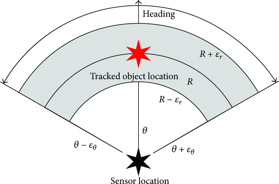
Terminology used to determine the portion of a circle arc that describes the valid sensor coverage area of a sensor.

Once the sensor parameters and constraints are known, the corresponding covariance matrix can be calculated using (1) with the variables defined as follows: n: sample size, $m_{xx}$ : $\left(r_i\cos t_i+x-{\mu }_x\right)\left(r_i\cos t_i+x-{\mu }_x\right)$ , $m_{yy}$ : $\left(r_i\sin t_i+y-{\mu }_y\right)\left(r_i\sin t_i+y-{\mu }_y\right)$ , $m_{xy}$ : $\left(r_i\cos t_i+x-{\mu }_x\right)\left(r_i\sin t_i+y-{\mu }_y\right)$ , $r_i$ : radius of the arc at point i, $t_i$ : angle of point i with respect to the sensor, x: X position of the sensor, y: Y position of the sensor, ${\mu }_x$ : mean x value, and ${\mu }_y$ : mean y value [13]. Consider

$$\begin{array}{cc}& \mathrm{cov}\left(x,y\right)=\frac{\mathrm{1}}{n-\mathrm{1}}{\displaystyle \sum }_{i=\mathrm{1}}^n\left[\begin{array}{cc}{m}_{xx}& m_{xy}\\ m_{xy}& m_{yy}\end{array}\right].\end{array}$$

(1)

This results in the following error covariance matrix where σ is the standard deviation:

$$\begin{array}{cc}& \mathrm{cov}\left(x,y\right)=\left[\begin{array}{cc}{\left(\sigma x\right)}^{\mathrm{2}}& \sigma xy\\ \sigma xy& {\left(\sigma y\right)}^{\mathrm{2}}\end{array}\right].\end{array}$$

(2)

This covariance matrix is then used to define the corresponding error ellipse.

The semimajor and semiminor axes of the error ellipses for each sensor are derived from the eigenvalues of their covariance matrices as shown in the following equations adapted from [14]:

$$\begin{array}{cc}& a=\sqrt{{\chi }_{\mathrm{2}}^{\mathrm{2}}·{\lambda }_{\mathrm{1}}},\\ b=\sqrt{{\chi }_{\mathrm{2}}^{\mathrm{2}}·{\lambda }_{\mathrm{2}}}.\end{array}$$

(3)

In (3), a is the semimajor axis of the error ellipse, b is the semiminor axis of the error ellipse, ${\lambda }_i$ are the eigenvalues of the covariance matrix found in (2), and ${\chi }_{\mathrm{2}}^{\mathrm{2}}$ is the chi-squared distribution with two degrees of freedom. In the case presented here, a 60% probability distribution was desired so the corresponding chi-squared value of 1.833 was found in [15]. The angle of rotation for the error ellipse was used solely for visualization purposes and was also determined from the covariance matrix. It is described by the following equation found in [16]:

$$\begin{array}{cc}& \omega =\frac{\mathrm{1}}{\mathrm{2}}\mathrm{ta}{\mathrm{n}}^{-\mathrm{1}}\left(\frac{\mathrm{2}\sigma xy}{{\left(\sigma y\right)}^{\mathrm{2}}-{\left(\sigma x\right)}^{\mathrm{2}}}\right).\end{array}$$

(4)

This angle is the counterclockwise rotation angle of the error ellipse with respect to the y-axis.

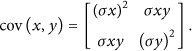
Once the error ellipse for each sensor in the experiment was determined, the next step was to find a combined error ellipse for all sensors in the system. Reference [16] showed that a combined error ellipse can be found as follows:

$$\begin{array}{cc}& \mathrm{cov}{\left(x,y\right)}_{\text{comb}}={\left({\displaystyle \sum }_{i=\mathrm{1}}^a{\left(\mathrm{cov}{\left(x,y\right)}_i\right)}^{-\mathrm{1}}\right)}^{-\mathrm{1}}.\end{array}$$

(5)

The semimajor and semiminor axes for this combined ellipse were then found using (3) as for the individual matrices. In all cases, the error ellipses were assumed to be centered on the tracked object. Figure 2 shows an example of two sensors and their resulting error ellipses, as well as the resulting combined error ellipse.

Figure 2

An example of the error ellipses. (a) shows the position of the sensors with respect to the tracked object. The guide shows that the sensors are, indeed, at a fixed radius from the tracked object. (b) shows the resulting error ellipses. The error ellipses are slanted in the direction specified by ω and the combined error ellipse is found using (5).

3. Optimization and Mathematical Simulation Results

The optimal geometric tracking configuration is found by minimizing the area of the combined ellipse, found by

$$\begin{array}{cc}& \text{Area}=\pi ab.\end{array}$$

(6)

Physically, the smaller the area for the combined error ellipse is, the closer the estimated location of the tracked object will be to the actual location. A closed-form expression for the area, with inputs of radii from the target, the tracking stations’ headings, the radial errors, and the angular errors, is found and optimized in Section 6.

The target and the mobile sensor systems were both constrained to move at a maximum speed of 0.315 m/s. Each time step in the following simulations and experiments was 0.125 s long so a maximum distance of less than 0.04 m could occur in each time step. Since this distance was on par with the error in the ultrawide band system used to provide the robot locations, the simplifying assumption was made that the optimal sensor system configuration could be determined as a static configuration for each time step with minimal loss of accuracy.

To test the optimization theory for veracity, two test cases were used; both were constrained to a fixed radius of 2.83 m from the tracked object. This distance was chosen because the optimal viewing distance for the quadrotors used in the physical experiments was between 1.7 m and 3.3 m. A viewing distance of 2.83 m was within the optimal viewing distance and allowed the quadrotors to be placed 2 m away from the target and 4 m apart. Case 1 featured two identical sensor systems while Case 2 featured one sensor system with a small angular error but a large radial error and one sensor system with a large angular error but a small radial error. The circular arcs corresponding to the sensors for both cases are shown in Figure 3. Both cases had been examined from a geometric perspective and Case 1 had been explored experimentally in work at Santa Clara University [17]. The smallest estimation error was found from a geometric perspective by finding the angle of separation between the sensor systems which resulted in the smallest area of overlapping valid sensor coverage areas when both sensors were pointed at the same target. It was found that Case 1 had an optimal sensor system separation of ±π/2 radians, as predicted by geometric considerations and [17]. The angle of separation has the same general configuration at π/2 radians and –π/2 radians; however, the positions of the individual sensor systems are reversed. Mathematically, these configurations are identical. This optimal configuration also matched that used by researchers in [7]. Case 2 was found to have an optimal separation angle of ±π radians as predicted by geometric considerations. Again, these two configurations are mathematically identical. This constitutes sufficient validation to test the theory in both simulation and physical experiments.

Figure 3

Test Case 1 (a) and Case 2 (b) sensor circular arcs. The sensor arcs in Case 1 are identical and are expected to have the lowest estimation error at a separation angle of π/2 radians. The sensor arcs in Case 2 have very different properties and are expected to have the lowest estimation error at a separation angle of π radians.

Note that a fixed radius was used for both tests because it allowed for the examination of the angle of separation between sensor systems without additional effects from changing multiple variables. A radius of 2.83 m was chosen for this initial test because it was both a distance that was practical for later experimental work at Santa Clara University and showed clear differentiation in the results at each separation angle. The examination of the effects of changing multiple parameters will be examined in future work.

3.1. Mathematical Simulation of Two Tracking Stations at a Fixed Radius with Identical Sensor Systems

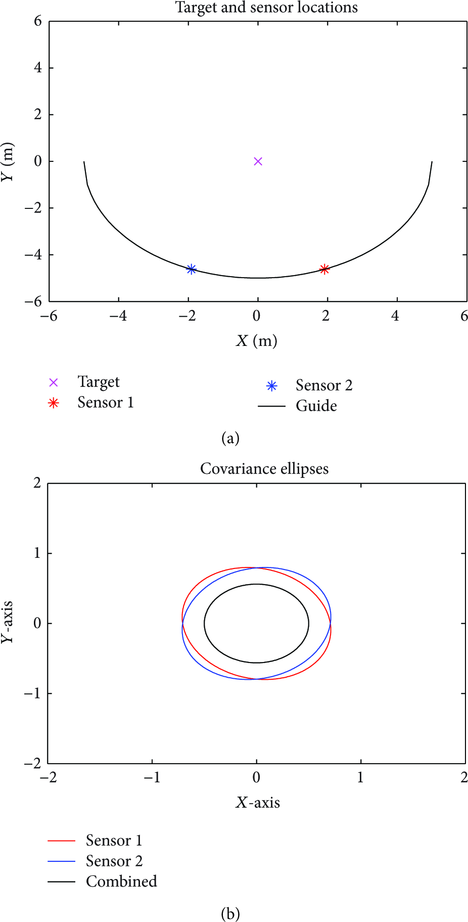
Equations (1) through (6) in the previous sections were used to mathematically simulate two tracking stations at a fixed radius of 2.83 m from the tracked object. The sensors for each tracking station were identical, as in Case 1, and were given an angular error of 0.1 radians and a radial error of 0.4 m to match the quadrotor sensor parameters. In the simulation, the tracking stations were separated by 0 through π radians and the resulting combined error ellipse area was found at each point. The curve formed by the area of the combined error ellipse at each angle of separation, shown in Figure 4, was found to have an ideal angle of separation of π/2 radians, as expected from [17] and Case 1.

Figure 4

Mathematical simulation results of two tracking stations with identical sensors at a fixed radius of 2.83 m from the tracked object. This plot shows the area of the combined error ellipse as a function of the angle of separation between the two mobile tracking stations.

This simulation was then repeated at a fixed radius of 30 m to test whether the same ideal angle of separation would be found at a much greater radius from the tracked object. The sensor error parameters remained the same: an angular error of 0.1 radians and a radial error of 0.4 m. Again, the angle of separation was varied from 0 to π radians in increments of π/18 radians and the combined ellipse area was found for each angle. The resulting curve can be seen in Figure 5 and illustrates the same ideal angle of separation of π/2 radians. There are two notable differences between this curve and that shown in Figure 4. First, the combined ellipses have much greater areas in Figure 5, as expected due to the much larger valid sensor coverage areas at greater distances. Secondly, the curve is much more rounded at greater distances and has a more nearly flat bottom. This is also expected since the valid sensor coverage areas are much wider than they are long so their overlapping coverage areas are very similar between π/3 radians and 2π/3 radians. However, this curve illustrates that the ideal angle of separation between two identical sensor systems is π/2 radians for a variety of ranges.

Figure 5

Mathematical simulation results of two tracking stations with identical sensors at a fixed radius of 30 m from the tracked object. This plot shows the area of the combined error ellipse as a function of the angle of separation between the two mobile tracking stations.

3.2. Mathematical Simulation of Two Tracking Stations at a Fixed Radius with Different Sensor Systems

The equations presented in the previous sections were also used to mathematically simulate the effect of two tracking stations with different sensor parameters at a fixed radius of 2.83 m. Sensor 1 was assigned an angular error of 0.1 radians and a radial error of 0.8 m while sensor 2 was given an angular error of 0.2 radians and a radial error of 0.4 m. Again, the tracking stations were separated by 0 to π radians with the resulting combined error ellipse area calculated at each point. Figure 6 shows the resultant curve, which was found to have an ideal angle of separation at 0 radians and π radians. A separation angle of 0 radians is physically impossible since the sensor systems cannot be collocated, but a separation of π radians represents the same configuration obtained from Case 2 in the previous section.

Figure 6

Mathematical simulation results of two tracking stations with different sensors at a fixed radius of 2.83 m from the tracked object. This plot shows the area of the combined error ellipse as a function of the angle of separation between the two mobile tracking stations.

Two tracking stations at a fixed radius of 30 m with different sensors were also mathematically simulated in order to verify that the same ideal angle of separation was valid. Sensor 1 was assigned an angular error of 0.1 radians and a radial error of 3.2 m while sensor 2 was assigned an angular error of 0.8 radians and a radial error of 0.4 m. These values were different from those used in the previous simulation because the valid sensor coverage areas were large enough that a greater magnitude change was necessary to create the significantly different sensors assumed in this scenario. The resulting curve can be seen in Figure 7. This is the same shape as seen in Figure 6 with the same ideal angles of separation of 0 radians and π radians. The only difference is that the area of the combined covariance ellipse is greater in magnitude at a distance of 30 m. This is expected due to the larger size of the valid sensor coverage areas themselves and the larger magnitude of the sensor errors. This simulation again confirms that this methodology applies to a variety of sensor ranges.

Figure 7

Mathematical simulation results of two tracking stations with different sensors at a fixed radius of 30 m from the tracked object. This plot shows the area of the combined error ellipses as a function of the angle of separation between the two mobile tracking stations.

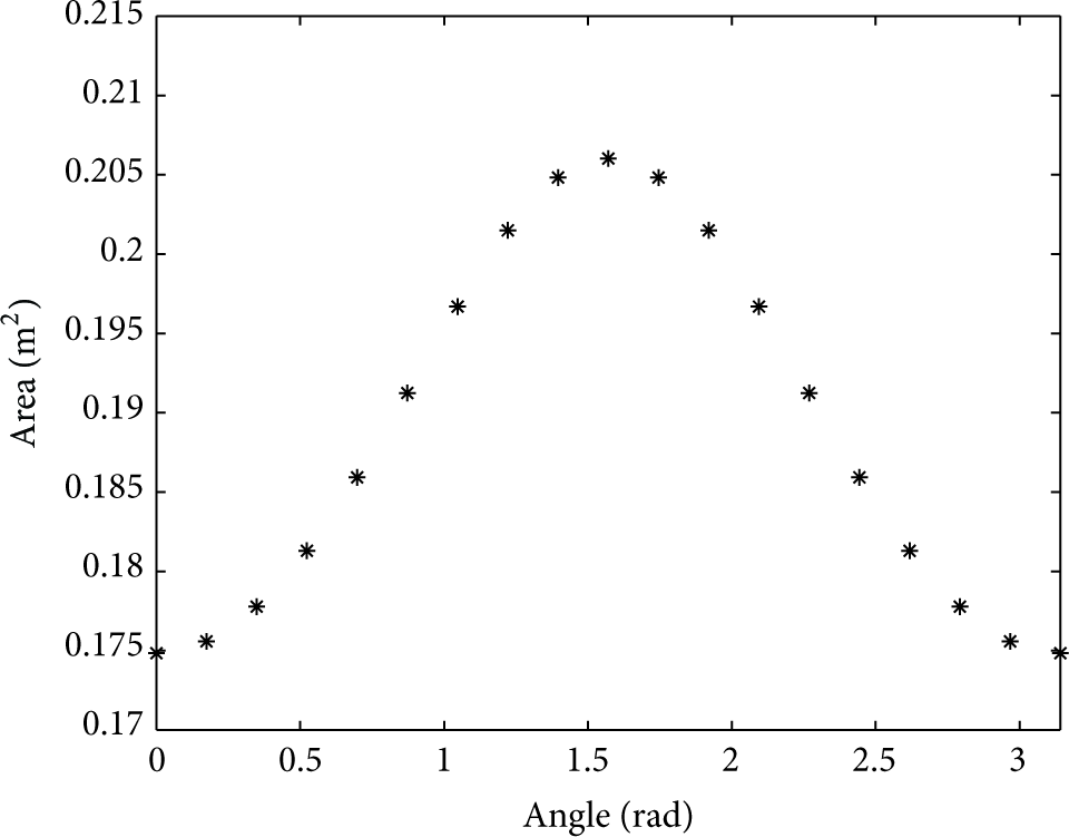
3.3. Mathematical Simulation of Three Tracking Stations at a Fixed Radius with Identical Sensor Systems

Equations (1) through (6) in the previous sections were also used to mathematically simulate three tracking stations at a fixed radius of 2.83 m from the tracked object. The sensor parameters were matched to the quadrotor sensor parameters: the angular error was 0.1 radians and the radial error was 0.4 m for each sensor. In all cases with three tracking stations, the first tracking station was placed directly in front of and facing the tracked object. The remaining two tracking stations were positioned symmetrically on either side of the first tracking station. The angle of separation was defined as the angle between the second and third tracking stations, as shown in Figure 8. In this simulation, the combined error ellipse area was found for angles of separation between 0 radians and 2π radians. The ideal angle of separation was found to be 2π/3 radians or 4π/3 radians, which both have the same effective angle of separation between sensor systems 2 and 3, although an angular separation of 2π/3 radians is easier to use in practice. The results of the mathematical simulation are shown in Figure 9.

Figure 8

Definition of the angle of separation for three tracking stations.

Figure 9

Mathematical simulation results of three tracking stations with the same sensors at a fixed radius of 2.83 m from the tracked object. This plot shows the area of the combined error ellipses as a function of the angle of separation between the three mobile tracking stations, as shown in Figure 8.

A variation of this simulation was also performed at a fixed radius of 2.83 m where each sensor system angle was varied separately, allowing for asymmetric angles of separation. This produced the contour plot shown in Figure 10. Here, there were two angles of separation: the angle between sensor system 2 and the static sensor system 1 and the angle between sensor system 3 and the static sensor system 1. These angles of separation were independent of one another. The lowest area of the combined ellipse occurred in eight places, marked by the smallest blue circles in Figure 10. These areas correspond to the following angle of separation couplets that represent sensor system 2 and sensor system 3 in radians: (2π/3, −2π/3), (−2π/3, 2π/3), (π/3, −π/3), (−π/3, π/3), (π/3, 2π/3), (−π/3, −2π/3), (2π/3, π/3), and (−2π/3, −π/3). Each of these combinations yielded an angle of separation between sensor systems 2 and 3, as defined in Figure 8, of ±2π/3 radians and represented the same effective geometric configuration. This confirms that the angle of separation was the global ideal and not simply an artifact of the definition of the angle of separation.

Figure 10

Mathematical simulation results of three tracking stations with the same sensors at a fixed radius of 2.83 m from the tracked object. This plot shows the area of the combined error ellipses as a function of the angle of separation between the three mobile tracking stations where each angle of separation is varied separately.

3.4. Mathematical Simulation of Three Tracking Stations at a Fixed Radius with Different Sensor Systems

Finally, (1) through (6) were used to mathematically simulate three tracking stations with different sensor systems at a fixed radius of 2.83 m from the tracked object. The angle of separation was again defined as in Figure 8 and only symmetric configurations were examined. Here, sensor 1 was given an angular error of 0.1 radians and a radial error of 0.4 m, sensor 2 was given an angular error of 0.1 radians and a radial error of 0.8 m, and sensor 3 was given an angular error of 0.2 radians and a radial error of 0.4 m. Again, the tracking stations were separated by 0 through 2π radians and the resulting area of the combined error ellipse was found. The ideal angle of separation was found to consist of a single value: π radians. Figure 11 shows the mathematical simulation results.

Figure 11

Mathematical simulation results of three tracking stations with different sensors at a fixed radius of 2.83 m from the tracked object. This plot shows the area of the combined error ellipse as a function of the angle of separation between the three mobile tracking stations, as shown in Figure 8.

A variation of this simulation was performed where each sensor system angle was varied independently to allow for asymmetric results. The same fixed radius of 2.83 m was used for all three sensor systems in this simulation, and the resulting contour plot can be seen in Figure 12. As in Section 3.3, the two independent angles of separation were defined as the angle between sensor 2 and sensor 1 and the angle between sensor 3 and sensor 1. The minimum of this plot occurred in four places, marked by the darkest blue circles in Figure 12, and was centered on the following couplets: (−π/2, −π/2), (π/2, π/2), (−π/2, π/2), and (π/2, −π/2). The first two couplets are not physically possible as the two sensor systems cannot be collocated, but the second two couplets both represent a separation angle of π radians, as was found in Figure 11. This further confirms that the ideal angle of separation was not merely an artifact of the definition of the angle of separation.

Figure 12

Mathematical simulation results of three tracking stations with different sensors at a fixed radius of 2.83 m from the tracked object. This plot shows the area of the combined error ellipses as a function of the angle of separation between the three mobile tracking stations where each angle of separation is varied separately.

3.5. Summary of Findings

The mathematical simulations in this section confirm that the ideal angle of separation calculations hold true for two and three robot configurations. This methodology can accommodate a variety of sensor system ranges and cases of both identical and nonidentical sensor systems. Specifically, the two robot results demonstrate that the ideal angle of separation is more heavily dependent on the relative sensor performance than on the radius between the sensor systems and the tracked object. The three drone cases with identical sensor systems verified that the ideal angle of separation of sensor systems is not an artifact of the definition of the angle of separation but is truly a property of the sensor systems themselves. The three drone cases with nonidentical sensor systems confirmed that the sensor properties affect the ideal angle of separation calculations.

4. Testbed

In the following experiments, the testbed described in [18] was used. In this testbed, the tracked object was a Pioneer 3-AT land rover robot, as seen in Figure 13. The Pioneer is 0.508 m long and 0.277 m wide and weighs 12 kg. It has a running time of 3 hours and a maximum speed of 0.7 m/s [19]. The mobile tracking stations were Parrot's AR.Drone 1.0 aerial robots. These quadrotors are 0.525 m by 0.515 m with the indoor hull shown in Figure 14 that was used for each of the experiments. They have a running time of 15 minutes and a maximum speed of 5 m/s with no payload [20].

Figure 13

Pioneer land rover used as the tracked object. A front view (a) and side view (b) are shown.

Figure 14

Parrot's AR.Drone 1.0 quadrotors were used as the mobile tracking stations. The front camera was used as the sensor to track the position of the Pioneer.

Additionally, the quadrotors have two RGB color cameras. The sensor used to estimate the position of the tracked object was the onboard front-mounted camera with a 93-degree wide-angle diagonal lens. The camera image is 240 by 320 pixels and is updated at a rate of 30 Hz [20]. The quadrotors located the Pioneer by its distinctive red color and the resulting image was simplified to allow for real-time data transmission on the quadrotors’ native WiFi network. Unfortunately, the quadrotors all used the same IP address, so separate computers were necessary for each robot.

The Sapphire Dart Ultrawide Band (UWB) tracking system was implemented in order to collect robot position data for the quadrotors and truth data for the Pioneer in this testbed. The UWB tracking system consisted of a series of receivers placed around the perimeter of the test area at various heights and radio frequency identification (RFID) tags, two of which were used as reference tags in the test area and two of which were placed on each robot. The RFID tags transmit at 25 Hz while the receivers triangulate the position of each tag [21]. Each robot, both quadrotors and the Pioneer, had two RFID tags attached: one on the robot's extreme right and one on its extreme left, the mean of which was used to calculate the robot's position. The two tags were also used to calculate the robot's heading. An image of an RFID tag and receiver can be seen in Figure 15 while a data flow diagram that illustrates how the various sensor readings and robot commands were passed through the system in this setup is shown in Figure 16.

Figure 15

An RFID tag and an UWB receiver, shown with a quarter for scale.

Figure 16

Data flow diagram for this testbed.

5. Experimental Results for Mobile Tracking Stations at a Fixed Radius

Next, two series of physical experiments were performed and compared to the mathematical results. Both series of physical experiments were performed with stationary quadrotors; to mimic actual flight conditions, the quadrotors were statically mounted at their nominal flight height. Configurations with separation angles of π/18 radians to π radians in increments of π/18 radians were evaluated at a fixed radius of 2.83 m. Data was collected for two minutes at each location and the mean total distance between the actual Pioneer position and the estimated Pioneer position was measured.

In the first series of experiments, the Pioneer itself was used as the tracked object and two quadrotors were used as the mobile tracking stations. The normalized results can be seen in Figure 17. The theoretical shape is the same as for the simulation results. Again, the general shape of the curve followed the theory. However, the angles below π/2 radians yielded a smaller change in the total distance error each time the angle of separation was changed than the theory predicted. This is believed to be because the RFID system errors have a larger relative effect on the position estimations at small distances between the sensor systems. Additionally, the angle of separation with the minimum mean total distance error was found to be 11π/18 radians rather than the predicted π/2 radians. The cause of this deviation was posited to be the shape of the Pioneer itself. Figure 13 shows that the Pioneer features large wheels that can obscure large portions of the body of the Pioneer.

Figure 17

Experimental results of two quadrotors at a fixed radius of 2.83 m from the tracked object. This plot shows the area of the combined error ellipse as a function of the angle of separation between the two mobile tracking stations.

To determine whether this feature was responsible for the difference between the theory and the experimental results, a second series of tests was performed with two tracking stations and a uniform object that looked the same when viewed from any angle. A red ball with an apparent surface area similar to the side of the Pioneer was chosen as the uniform object. Figure 18 shows the Pioneer from the front and side next to this uniform object. The normalized results from this series of experiments are also shown in Figure 17 and exhibit the same shape as the theoretical curve with the same lower slope at angles of separation below π/2 radians. However, the angle of separation that produced the minimum mean total distance error was found to be 5π/9 radians which is much closer to the theoretical minimum of π/2 radians, suggesting that the shift observed in the first series of physical experiments was mainly due to the shape of the Pioneer itself. The remaining deviation from theory is thought to be caused by the lack of uniform lighting in the test area and an exploration of this theory is suggested for future work.

Figure 18

The uniform object next to the Pioneer front view (a) and side view (b).

A third series of experiments was conducted using three quadrotors as the mobile tracking stations and the Pioneer as the tracked object. The normalized results can be seen in Figure 19. These physical results initially showed a slower decrease in the area of the combined ellipse per change in angle of separation than predicted by theory but resulted in a similar minimum value of 5π/6 radians. As in the two quadrotor cases, the discrepancy between the theoretical minimum of 2π/3 radians and the experimental minimum of 5π/6 radians was believed to be due to the shape of the Pioneer. After reaching this minimum value, the area of the combined error ellipse increased more sharply than predicted by the theory. This is thought to be because of differences in the background of the test environment. Testing in an area with uniformly painted walls and uniformly distributed building structures is recommended for future work.

Figure 19

Experimental results of three quadrotors at a fixed radius of 2.83 m from the tracked object. This plot shows the area of the combined error ellipse as a function of the angle of separation between the three mobile tracking stations, as shown in Figure 8.

To verify that a uniform object would yield a minimum closer to the theoretical minimum, a final series of physical experiments were performed using three static quadrotors as the mobile tracking stations and a uniform object, a red ball, as the tracked object. The results of these experiments are also shown in Figure 19 and demonstrate a smooth decrease down to a minimum value of 2π/3 radians and then a sharper increase in the area of the combined error ellipse than predicted by the theory. However, the minimum found by this series of experiments was the same as the theoretical minimum of 2π/3 radians, unlike when the Pioneer was used as the tracked object. This confirms that most of the discrepancy in the minimum was due to the shape of the Pioneer.

The application domain for this methodology assumes a maximum target speed of 0.315 m/s in the 19 by 12 m test area. Two solutions are presented here: one solution for the case with two mobile sensor systems and one solution for the case with three sensor systems. The case with two sensor systems resulted in a mean error of 0.68 m for the experimental results with the Pioneer. For the three sensor system case, the mean experimental error was even less at 0.6 m. This accuracy is sufficient to keep the object in view of the sensing systems, allowing for continued tracking of the object.

In general, the experimental results were found to match the theory within physical limitations. In the worst case scenario, two quadrotors with a separation angle of π radians tracking a Pioneer, the mean total distance error was less than 1.5 m. This distance was less than the field of view of the quadrotors at a distance of 2.83 m from the tracked object, meaning that the Pioneer could still be correctly located even after such a large estimation error. The best case scenario for the experimental results, three quadrotors with a separation angle of 2π/3 radians tracking a ball, had a mean total distance error of 0.1 m which was very close in a test area measuring approximately 19 m by 12 m.

6. Optimization

In the previous sections, (1) through (6) were shown to match real-world results. In this section, these equations are combined to obtain a single closed-form expression that can be formally optimized. Rather than calculating separate covariance matrices for each sensor heading, a single covariance matrix was calculated for each sensor at a heading of zero radians and a single fixed radius. This covariance matrix was then rotated to the desired heading using the matrix rotation formula shown in

$$\begin{array}{l}{\left.\left[\begin{array}{ll}{\left(\sigma x\right)}^{\mathrm{2}}& \sigma xy\\ \sigma xy& {\left(\sigma y\right)}^{\mathrm{2}}\end{array}\right]\right|}_{\theta }\\ =\left[\begin{array}{ll}\cos \left(\theta \right)& -\sin \left(\theta \right)\\ \sin \left(\theta \right)& \cos \left(\theta \right)\end{array}\right]\\ \ast \left[\begin{array}{ll}{\left(\sigma x\right)}^{\mathrm{2}}& \sigma xy\\ \sigma xy& {\left(\sigma y\right)}^{\mathrm{2}}\end{array}\right]\left[\begin{array}{ll}\cos \left(\theta \right)& \sin \left(\theta \right)\\ -\sin \left(\theta \right)& \cos \left(\theta \right)\end{array}\right].\end{array}$$

(7)

The matrix rotation formula used in (7) is a standard formula in dynamics and can be used in this application since x and y were independent variables.

Next, the sensor covariance matrix at a heading of zero radians was calculated symbolically. It was assumed that x and y were products of the independent random variables r (range to the target) and t (heading to the target), which were assumed to have a uniform distribution. Thus

$$\begin{array}{cc}& x=r_i\cos \left(t_i\right)+x_{\text{ts}n}-{\mu }_x,\\ y=r_i\sin \left(t_i\right)+y_{\text{ts}n}-{\mu }_y.\end{array}$$

(8)

Here, $x_{\text{ts}n}$ is the x location of tracking station n, ${\mu }_x$ is the average x position of tracking station n, $y_{\text{ts}n}$ is the y location of tracking station n, and ${\mu }_y$ is the average y position of tracking station n. At a heading of zero radians, $x_{\text{ts}n}-{\mu }_x$ simplifies to R, the radius from the tracking station to the tracked object, and $y_{\text{ts}n}-{\mu }_y$ simplifies to 0. This is due to the symmetric distribution of the valid sensing area about the target object and results in the following simplified equations:

$$\begin{array}{cc}& x=r_i\cos \left(t_i\right)+R,\\ y=r_i\sin \left(t_i\right).\end{array}$$

(9)

However, since the variance of $Z+q$ when q is a constant and Z is a variable is the same as the variance of Z by the properties of variance [22], the equation for x, for the purpose of calculating the variance only, can be further reduced to

$$\begin{array}{cc}& x=r_i\cos \left(t_i\right).\end{array}$$

(10)

At a fixed heading of zero radians, the values of $r_i$ and $t_i$ are dependent on the radius of the tracked object from the tracking station, the radial error, and the angular error of the tracking station. Consequently, the values of the covariance matrix can be found as follows:

$$\begin{array}{l}{\left(\sigma x\right)}^{\mathrm{2}}=E\left(x_{\mathrm{1}}^{\mathrm{2}}\right)E\left(x_{\mathrm{2}}^{\mathrm{2}}\right)-{\left(E\left(x_{\mathrm{1}}\right)\right)}^{\mathrm{2}}{\left(E\left(\left(x_{\mathrm{2}}\right)\right)\right)}^{\mathrm{2}}\\ =E\left(r^{\mathrm{2}}\right)E\left({\cos }^{\mathrm{2}}\left(\theta \right)\right)-{\left(E\left(r\right)\right)}^{\mathrm{2}}{\left(E\left(\cos \left(\theta \right)\right)\right)}^{\mathrm{2}}\\ =\left({{\displaystyle \int }}_{R-{\epsilon }_r}^{R+{\epsilon }_r}\left(\frac{r^{\mathrm{2}}}{R+{\epsilon }_r-\left(R-{\epsilon }_r\right)}\right)dr\right)\\ \ast \left({{\displaystyle \int }}_{-{\epsilon }_{\theta }}^{{\epsilon }_{\theta }}\left(\frac{{\cos }^{\mathrm{2}}\left(\theta \right)}{{\epsilon }_{\theta }-\left(-{\epsilon }_{\theta }\right)}\right)d\theta \right)\\ -{\left({{\displaystyle \int }}_{R-{\epsilon }_r}^{R+{\epsilon }_r}\left(\frac{r}{R+{\epsilon }_r-\left(R-{\epsilon }_r\right)}\right)dr\right)}^{\mathrm{2}}\\ \ast {\left({{\displaystyle \int }}_{-{\epsilon }_{\theta }}^{{\epsilon }_{\theta }}\left(\frac{\cos \left(\theta \right)}{{\epsilon }_{\theta }-\left(-{\epsilon }_{\theta }\right)}\right)d\theta \right)}^{\mathrm{2}}\\ =\left(R^{\mathrm{2}}+\frac{{\epsilon }_r^{\mathrm{2}}}{\mathrm{3}}\right)\frac{\mathrm{1}}{\mathrm{2}{\epsilon }_{\theta }}\left({\epsilon }_{\theta }+\frac{\mathrm{1}}{\mathrm{2}}\sin \left(\mathrm{2}{\epsilon }_{\theta }\right)\right)\\ -\frac{R^{\mathrm{2}}}{{\epsilon }_{\theta }^{\mathrm{2}}}{\sin }^{\mathrm{2}}\left({\epsilon }_{\theta }\right).\end{array}$$

(11)

In this equation, $x_1=r$ and $x_2=\cos (\theta )$ . Consider

$$\begin{array}{l}{\left(\sigma y\right)}^{\mathrm{2}}=E\left(y_{\mathrm{1}}^{\mathrm{2}}\right)E\left(y_{\mathrm{2}}^{\mathrm{2}}\right)-{\left(E\left(y_{\mathrm{1}}\right)\right)}^{\mathrm{2}}{\left(E\left(\left(y_{\mathrm{2}}\right)\right)\right)}^{\mathrm{2}}\\ =E\left(r^{\mathrm{2}}\right)E\left({\sin }^{\mathrm{2}}\left(\theta \right)\right)-{\left(E\left(r\right)\right)}^{\mathrm{2}}{\left(E\left(\sin \left(\theta \right)\right)\right)}^{\mathrm{2}}\\ =\left({{\displaystyle \int }}_{R-{\epsilon }_r}^{R+{\epsilon }_r}\left(\frac{r^{\mathrm{2}}}{R+{\epsilon }_r-\left(R-{\epsilon }_r\right)}\right)dr\right)\\ \ast \left({{\displaystyle \int }}_{-{\epsilon }_{\theta }}^{{\epsilon }_{\theta }}\left(\frac{{\sin }^{\mathrm{2}}\left(\theta \right)}{{\epsilon }_{\theta }-\left(-{\epsilon }_{\theta }\right)}\right)d\theta \right)\\ -{\left({{\displaystyle \int }}_{R-{\epsilon }_r}^{R+{\epsilon }_r}\left(\frac{r}{R+{\epsilon }_r-\left(R-{\epsilon }_r\right)}\right)dr\right)}^{\mathrm{2}}\\ \ast {\left({{\displaystyle \int }}_{-{\epsilon }_{\theta }}^{{\epsilon }_{\theta }}\left(\frac{\sin \left(\theta \right)}{{\epsilon }_{\theta }-\left(-{\epsilon }_{\theta }\right)}\right)d\theta \right)}^{\mathrm{2}}\\ =\left(R^{\mathrm{2}}+\frac{{\epsilon }_r^{\mathrm{2}}}{\mathrm{3}}\right)\frac{\mathrm{1}}{\mathrm{2}{\epsilon }_{\theta }}\left({\epsilon }_{\theta }-\frac{\mathrm{1}}{\mathrm{2}}\sin \left(\mathrm{2}{\epsilon }_{\theta }\right)\right).\end{array}$$

(12)

In (12), $y_1=r$ and $y_2=\sin (\theta )$ . Consider

$$\begin{array}{l}(\sigma xy)=E(xy)-E(x)*(y)\hfill \\ ={\int }_{R-{\varepsilon }_r}^{R+{\varepsilon }_r}{\int }_{-{\varepsilon }_{\theta }}^{{\varepsilon }_{\theta }}\frac{1}{2{\varepsilon }_{\theta }}\frac{1}{2{\varepsilon }_r}(r^{2}sin(\theta )cos(\theta )\hfill \\ +Rrsin(\theta ))d\theta dr\hfill \\ -\left(={\int }_{R-{\varepsilon }_r}^{R+{\varepsilon }_r}{\int }_{-{\varepsilon }_{\theta }}^{{\varepsilon }_{\theta }}\frac{1}{2{\varepsilon }_{\theta }}\frac{1}{2{\varepsilon }_r}(rcos(\theta )+R)d\theta dr\right)\hfill \\ *\left(={\int }_{R-{\varepsilon }_r}^{R+{\varepsilon }_r}{\int }_{-{\varepsilon }_{\theta }}^{{\varepsilon }_{\theta }}\frac{1}{2{\varepsilon }_{\theta }}\frac{1}{2{\varepsilon }_r}(rsin(\theta ))d\theta dr\right)=0-R\hfill \\ *0=0.\hfill \end{array}$$

(13)

These equations allow for the direct calculation of the covariance matrix for each sensor system as shown in (2).

Next, the individual covariance matrices were rotated as shown in (7) and substituted into (5) to obtain the combined covariance matrix. The resulting equation allows for the direct calculation of this combined covariance matrix using only the tracking stations’ radii, headings, and associated errors, reducing the number of calculations necessary. For the case with two tracking stations, the combined covariance matrix can be directly calculated using the following equations:

$$\begin{array}{l}\mathrm{cov}{\left(x,y\right)}_{\text{comb}}\\ =\frac{{\left(\sigma x\right)}_{\mathrm{1}}^{\mathrm{2}}{\left(\sigma y\right)}_{\mathrm{1}}^{\mathrm{2}}{\left(\sigma x\right)}_{\mathrm{2}}^{\mathrm{2}}{\left(\sigma y\right)}_{\mathrm{2}}^{\mathrm{2}}}{AC-B^{\mathrm{2}}}\ast \left[\begin{array}{ll}C& -B\\ -B& A\end{array}\right],\end{array}$$

(14)

$$\begin{array}{l}A\\ ={\left(\sigma x\right)}_{\mathrm{2}}^{\mathrm{2}}{\left(\sigma y\right)}_{\mathrm{2}}^{\mathrm{2}}\left({\sin }^{\mathrm{2}}\left({\theta }_{\mathrm{1}}\right){\left(\sigma x\right)}_{\mathrm{1}}^{\mathrm{2}}+{\cos }^{\mathrm{2}}\left({\theta }_{\mathrm{1}}\right){\left(\sigma y\right)}_{\mathrm{1}}^{\mathrm{2}}\right)\\ +{\left(\sigma x\right)}_{\mathrm{1}}^{\mathrm{2}}{\left(\sigma y\right)}_{\mathrm{1}}^{\mathrm{2}}\left({\sin }^{\mathrm{2}}\left({\theta }_{\mathrm{2}}\right){\left(\sigma x\right)}_{\mathrm{2}}^{\mathrm{2}}+{\cos }^{\mathrm{2}}\left({\theta }_{\mathrm{2}}\right){\left(\sigma y\right)}_{\mathrm{2}}^{\mathrm{2}}\right),\end{array}$$

(15)

$$\begin{array}{l}B\\ =\sin \left({\theta }_{\mathrm{1}}\right)\cos \left({\theta }_{\mathrm{1}}\right){\left(\sigma x\right)}_{\mathrm{2}}^{\mathrm{2}}{\left(\sigma y\right)}_{\mathrm{2}}^{\mathrm{2}}\left({\left(\sigma y\right)}_{\mathrm{1}}^{\mathrm{2}}-{\left(\sigma x\right)}_{\mathrm{1}}^{\mathrm{2}}\right)\\ +\sin \left({\theta }_{\mathrm{2}}\right)\cos \left({\theta }_{\mathrm{2}}\right){\left(\sigma x\right)}_{\mathrm{1}}^{\mathrm{2}}{\left(\sigma y\right)}_{\mathrm{1}}^{\mathrm{2}}\left({\left(\sigma y\right)}_{\mathrm{2}}^{\mathrm{2}}-{\left(\sigma x\right)}_{\mathrm{2}}^{\mathrm{2}}\right),\end{array}$$

(16)

$$\begin{array}{l}C\\ ={\left(\sigma x\right)}_{\mathrm{2}}^{\mathrm{2}}{\left(\sigma y\right)}_{\mathrm{2}}^{\mathrm{2}}\left({\cos }^{\mathrm{2}}\left({\theta }_{\mathrm{1}}\right){\left(\sigma x\right)}_{\mathrm{1}}^{\mathrm{2}}+{\sin }^{\mathrm{2}}\left({\theta }_{\mathrm{1}}\right){\left(\sigma y\right)}_{\mathrm{1}}^{\mathrm{2}}\right)\\ +{\left(\sigma x\right)}_{\mathrm{1}}^{\mathrm{2}}{\left(\sigma y\right)}_{\mathrm{1}}^{\mathrm{2}}\left({\cos }^{\mathrm{2}}\left({\theta }_{\mathrm{2}}\right){\left(\sigma x\right)}_{\mathrm{2}}^{\mathrm{2}}+{\sin }^{\mathrm{2}}\left({\theta }_{\mathrm{2}}\right){\left(\sigma y\right)}_{\mathrm{2}}^{\mathrm{2}}\right).\end{array}$$

(17)

For the case with three tracking stations, the combined covariance matrix can be similarly calculated using

$$\begin{array}{l}\mathrm{cov}{\left(x,y\right)}_{\text{comb}}\\ =\frac{{\left(\sigma x\right)}_{\mathrm{1}}^{\mathrm{2}}{\left(\sigma y\right)}_{\mathrm{1}}^{\mathrm{2}}{\left(\sigma x\right)}_{\mathrm{2}}^{\mathrm{2}}{\left(\sigma y\right)}_{\mathrm{2}}^{\mathrm{2}}{\left(\sigma x\right)}_{\mathrm{3}}^{\mathrm{2}}{\left(\sigma y\right)}_{\mathrm{3}}^{\mathrm{2}}}{GH-K^{\mathrm{2}}}\\ \ast \left[\begin{array}{ll}H& -K\\ -K& G\end{array}\right],\end{array}$$

(18)

$$\begin{array}{l}G\\ ={\left(\sigma x\right)}_{\mathrm{2}}^{\mathrm{2}}{\left(\sigma y\right)}_{\mathrm{2}}^{\mathrm{2}}{\left(\sigma x\right)}_{\mathrm{3}}^{\mathrm{2}}{\left(\sigma y\right)}_{\mathrm{3}}^{\mathrm{2}}\\ \ast \left({\sin }^{\mathrm{2}}\left({\theta }_{\mathrm{1}}\right){\left(\sigma x\right)}_{\mathrm{1}}^{\mathrm{2}}+{\cos }^{\mathrm{2}}\left({\theta }_{\mathrm{1}}\right){\left(\sigma y\right)}_{\mathrm{1}}^{\mathrm{2}}\right)\\ +{\left(\sigma x\right)}_{\mathrm{1}}^{\mathrm{2}}{\left(\sigma y\right)}_{\mathrm{1}}^{\mathrm{2}}{\left(\sigma x\right)}_{\mathrm{3}}^{\mathrm{2}}{\left(\sigma y\right)}_{\mathrm{3}}^{\mathrm{2}}\\ \ast \left({\sin }^{\mathrm{2}}\left({\theta }_{\mathrm{2}}\right){\left(\sigma x\right)}_{\mathrm{2}}^{\mathrm{2}}+{\cos }^{\mathrm{2}}\left({\theta }_{\mathrm{2}}\right){\left(\sigma y\right)}_{\mathrm{2}}^{\mathrm{2}}\right)\\ +{\left(\sigma x\right)}_{\mathrm{1}}^{\mathrm{2}}{\left(\sigma y\right)}_{\mathrm{1}}^{\mathrm{2}}{\left(\sigma x\right)}_{\mathrm{2}}^{\mathrm{2}}{\left(\sigma y\right)}_{\mathrm{2}}^{\mathrm{2}}\\ \ast \left({\sin }^{\mathrm{2}}\left({\theta }_{\mathrm{3}}\right){\left(\sigma x\right)}_{\mathrm{3}}^{\mathrm{2}}+{\cos }^{\mathrm{2}}\left({\theta }_{\mathrm{3}}\right){\left(\sigma y\right)}_{\mathrm{3}}^{\mathrm{2}}\right),\end{array}$$

(19)

$$\begin{array}{l}K\\ =\sin \left({\theta }_{\mathrm{1}}\right)\cos \left({\theta }_{\mathrm{1}}\right){\left(\sigma x\right)}_{\mathrm{2}}^{\mathrm{2}}{\left(\sigma y\right)}_{\mathrm{2}}^{\mathrm{2}}{\left(\sigma x\right)}_{\mathrm{3}}^{\mathrm{2}}{\left(\sigma y\right)}_{\mathrm{3}}^{\mathrm{2}}\\ \ast \left({\left(\sigma y\right)}_{\mathrm{1}}^{\mathrm{2}}-{\left(\sigma x\right)}_{\mathrm{1}}^{\mathrm{2}}\right)+\sin \left({\theta }_{\mathrm{2}}\right)\cos \left({\theta }_{\mathrm{2}}\right)\\ \ast {\left(\sigma x\right)}_{\mathrm{1}}^{\mathrm{2}}{\left(\sigma y\right)}_{\mathrm{1}}^{\mathrm{2}}{\left(\sigma x\right)}_{\mathrm{3}}^{\mathrm{2}}{\left(\sigma y\right)}_{\mathrm{3}}^{\mathrm{2}}\ast \left({\left(\sigma y\right)}_{\mathrm{2}}^{\mathrm{2}}-{\left(\sigma x\right)}_{\mathrm{2}}^{\mathrm{2}}\right)\\ +\sin \left({\theta }_{\mathrm{3}}\right)\cos \left({\theta }_{\mathrm{3}}\right){\left(\sigma x\right)}_{\mathrm{1}}^{\mathrm{2}}{\left(\sigma y\right)}_{\mathrm{1}}^{\mathrm{2}}{\left(\sigma x\right)}_{\mathrm{2}}^{\mathrm{2}}{\left(\sigma y\right)}_{\mathrm{2}}^{\mathrm{2}}\\ \ast \left({\left(\sigma y\right)}_{\mathrm{3}}^{\mathrm{2}}-{\left(\sigma x\right)}_{\mathrm{3}}^{\mathrm{2}}\right),\end{array}$$

(20)

$$\begin{array}{l}H\\ ={\left(\sigma x\right)}_{\mathrm{2}}^{\mathrm{2}}{\left(\sigma y\right)}_{\mathrm{2}}^{\mathrm{2}}{\left(\sigma x\right)}_{\mathrm{3}}^{\mathrm{2}}{\left(\sigma y\right)}_{\mathrm{3}}^{\mathrm{2}}\\ \ast \left({\cos }^{\mathrm{2}}\left({\theta }_{\mathrm{1}}\right){\left(\sigma x\right)}_{\mathrm{1}}^{\mathrm{2}}+{\sin }^{\mathrm{2}}\left({\theta }_{\mathrm{1}}\right){\left(\sigma y\right)}_{\mathrm{1}}^{\mathrm{2}}\right)\\ +{\left(\sigma x\right)}_{\mathrm{1}}^{\mathrm{2}}{\left(\sigma y\right)}_{\mathrm{1}}^{\mathrm{2}}{\left(\sigma x\right)}_{\mathrm{3}}^{\mathrm{2}}{\left(\sigma y\right)}_{\mathrm{3}}^{\mathrm{2}}\\ \ast \left({\cos }^{\mathrm{2}}\left({\theta }_{\mathrm{2}}\right){\left(\sigma x\right)}_{\mathrm{2}}^{\mathrm{2}}+{\sin }^{\mathrm{2}}\left({\theta }_{\mathrm{2}}\right){\left(\sigma y\right)}_{\mathrm{2}}^{\mathrm{2}}\right)\\ +{\left(\sigma x\right)}_{\mathrm{1}}^{\mathrm{2}}{\left(\sigma y\right)}_{\mathrm{1}}^{\mathrm{2}}{\left(\sigma x\right)}_{\mathrm{2}}^{\mathrm{2}}{\left(\sigma y\right)}_{\mathrm{2}}^{\mathrm{2}}\\ \ast \left({\cos }^{\mathrm{2}}\left({\theta }_{\mathrm{3}}\right){\left(\sigma x\right)}_{\mathrm{3}}^{\mathrm{2}}+{\sin }^{\mathrm{2}}\left({\theta }_{\mathrm{3}}\right){\left(\sigma y\right)}_{\mathrm{3}}^{\mathrm{2}}\right).\end{array}$$

(21)

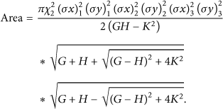
Next, the eigenvalues were found for (14) and the corresponding semimajor and semiminor axes were found using (3). These values were then substituted into (6) to obtain a single objective function for two tracking stations that could be minimized in order to find the optimal tracking configuration:

$$\begin{array}{l}\text{Area}=\frac{\pi {\chi }_{\mathrm{2}}^{\mathrm{2}}{\left(\sigma x\right)}_{\mathrm{1}}^{\mathrm{2}}{\left(\sigma y\right)}_{\mathrm{1}}^{\mathrm{2}}{\left(\sigma x\right)}_{\mathrm{2}}^{\mathrm{2}}{\left(\sigma y\right)}_{\mathrm{2}}^{\mathrm{2}}}{\mathrm{2}\left(AC-B^{\mathrm{2}}\right)}\\ \ast \sqrt{A+C+\sqrt{{\left(A-C\right)}^{\mathrm{2}}+\mathrm{4}{B}^{\mathrm{2}}}}\\ \ast \sqrt{A+C-\sqrt{{\left(A-C\right)}^{\mathrm{2}}+\mathrm{4}{B}^{\mathrm{2}}}}.\end{array}$$

(22)

Here, A, B, and C are defined by (15) through (17). For the case with three tracking stations, the eigenvalues from (18) were substituted into (6) to obtain a single objective function that could be minimized to find the optimal tracking configuration with three tracking stations as seen in

$$\begin{array}{l}\text{Area}=\frac{\pi {\chi }_{\mathrm{2}}^{\mathrm{2}}{\left(\sigma x\right)}_{\mathrm{1}}^{\mathrm{2}}{\left(\sigma y\right)}_{\mathrm{1}}^{\mathrm{2}}{\left(\sigma x\right)}_{\mathrm{2}}^{\mathrm{2}}{\left(\sigma y\right)}_{\mathrm{2}}^{\mathrm{2}}{\left(\sigma x\right)}_{\mathrm{3}}^{\mathrm{2}}{\left(\sigma y\right)}_{\mathrm{3}}^{\mathrm{2}}}{\mathrm{2}\left(GH-K^{\mathrm{2}}\right)}\\ \ast \sqrt{G+H+\sqrt{{\left(G-H\right)}^{\mathrm{2}}+\mathrm{4}{K}^{\mathrm{2}}}}\\ \ast \sqrt{G+H-\sqrt{{\left(G-H\right)}^{\mathrm{2}}+\mathrm{4}{K}^{\mathrm{2}}}}.\end{array}$$

(23)

Here, G, H, and K are defined in (19) through (21). In both (22) and (23), ${\chi }_{\mathrm{2}}^{\mathrm{2}}$ is the chi-squared distribution with two degrees of freedom as used in (3). Equations (22) and (23) were optimized using a constrained Hooke and Jeeves method [23], and the results were as expected: (22) had a minimum at an angle of separation of π/2 radians and (23) had a minimum at an angle of separation of 2π/3 radians. This further confirmed that the values found in the previous sections result in the minimum area of the combined error ellipse.

The Hooke and Jeeves method has the added benefit that its computation time scales linearly with the number of inputs [23]; the space complexity is $O(n)$ , so the number of robots can easily be increased. Specifically, the two robot cases presented here were computed on a conventional Pentium-class workstation with a 2.10 GHz processor and 4.00 GB of RAM in about 0.14 seconds while the result for the three robot cases was computed in 0.33 seconds. Both of these computation times are more than fast enough to correct a system under disturbances such as loss of a sensor system, changing sensor properties, or changing radii. If faster response times are desired, it is possible to precompute the optimal angle of separation for likely scenarios, reserving online computations for unforeseen changes.

7. Method Comparison

Compared to the symmetric, nonoptimized worst case examined by this research, the optimization method presented here results in a 6% target estimation improvement for both the two and the three fixed radius, identical sensor cases. This represents a significant improvement in the estimation of a target's location.

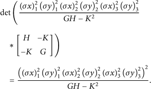
The method of sensor placement examined in this research was also compared to existing sensor placement optimization methods. Although similar to the method presented in [9], it cannot be directly compared since [9] assumes a covariance matrix produced by a Kalman filter. The method presented here does not use a Kalman filter, so the algorithm developed in [9] does not apply. Instead, this method is compared with the method presented in [24, 25] where the determinant of the error covariance matrix was minimized. In this method, the global covariance matrix was defined as follows:

$$\begin{array}{cc}& \det \left(P_{\text{global}}\right)=\det \left({\left({\displaystyle \sum }_{i=\mathrm{1}}^n{P}_i^{-\mathrm{1}}\right)}^{-\mathrm{1}}\right).\end{array}$$

(24)

Here, n is the total number of sensor systems and P is the error covariance matrix. Since $P_{\text{global}}$ is defined as in (5), a direct comparison between the methods can be found, for two mobile tracking stations, by taking the determinant of (14) in the previous section:

$$\begin{array}{l}\det \left(\frac{{\left(\sigma x\right)}_{\mathrm{1}}^{\mathrm{2}}{\left(\sigma y\right)}_{\mathrm{1}}^{\mathrm{2}}{\left(\sigma x\right)}_{\mathrm{2}}^{\mathrm{2}}{\left(\sigma y\right)}_{\mathrm{2}}^{\mathrm{2}}}{AC-B^{\mathrm{2}}}\ast \left[\begin{array}{ll}C& -B\\ -B& A\end{array}\right]\right)\\ =\frac{{\left({\left(\sigma x\right)}_{\mathrm{1}}^{\mathrm{2}}{\left(\sigma y\right)}_{\mathrm{1}}^{\mathrm{2}}{\left(\sigma x\right)}_{\mathrm{2}}^{\mathrm{2}}{\left(\sigma y\right)}_{\mathrm{2}}^{\mathrm{2}}\right)}^{\mathrm{2}}}{AC-B^{\mathrm{2}}}.\end{array}$$

(25)

In the case of a fixed radius and identical sensor systems examined here, (11) and (12) show that ${\left(\sigma x\right)}_{\mathrm{1}}^{\mathrm{2}}={\left(\sigma x\right)}_{\mathrm{2}}^{\mathrm{2}}$ and ${\left(\sigma y\right)}_{\mathrm{1}}^{\mathrm{2}}={\left(\sigma y\right)}_{\mathrm{2}}^{\mathrm{2}}$ for the fixed radius, identical sensor system case. Finally, the assumption can be made that ${\theta }_1=-{\theta }_2$ since any symmetric separation of angles yields the same result in the method presented here. Thus, $AC-B^2$ reduces to

$$\begin{array}{cc}& AC-B^{\mathrm{2}}=\mathrm{2}{\left(\sigma x\right)}^{\mathrm{2}}{\left(\sigma y\right)}^{\mathrm{2}}\left({\left(\sigma x\right)}^{\mathrm{2}}+{\left(\sigma y\right)}^{\mathrm{2}}\right).\end{array}$$

(26)

Equation (26) consists only of ${\left(\sigma x\right)}^{\mathrm{2}}$ and ${\left(\sigma y\right)}^{\mathrm{2}}$ terms, which were shown in the previous section to always have the same value. Thus, no minimum can be found for the fixed radius, identical sensor system case using the determinate method presented in [24, 25].

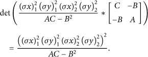
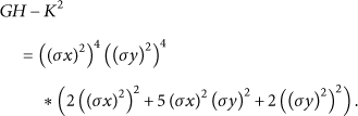
The fixed radius, identical sensor system, three mobile tracking stations’ case was also compared to the determinate method by taking the determinate of the matrix found in (18) from the previous section:

$$\begin{array}{l}\det (\frac{{\left(\alpha x\right)}_{\mathrm{1}}^{\mathrm{2}}{\left(\alpha y\right)}_{\mathrm{1}}^{\mathrm{2}}{\left(\alpha x\right)}_{\mathrm{2}}^{\mathrm{2}}{\left(\alpha y\right)}_{\mathrm{2}}^{\mathrm{2}}{\left(\alpha x\right)}_{\mathrm{3}}^{\mathrm{2}}{\left(\alpha y\right)}_{\mathrm{3}}^{\mathrm{2}}}{GH-K^{\mathrm{2}}}\\ *\left[\begin{array}{ll}\hspace{0.17em}H& -K\\ -K& G\end{array}\right])\\ =\frac{{\left({\left(\alpha x\right)}_{\mathrm{1}}^{\mathrm{2}}{\left(\alpha y\right)}_{\mathrm{1}}^{\mathrm{2}}{\left(\alpha x\right)}_{\mathrm{2}}^{\mathrm{2}}{\left(\alpha y\right)}_{\mathrm{2}}^{\mathrm{2}}{\left(\alpha x\right)}_{\mathrm{3}}^{\mathrm{2}}{\left(\alpha y\right)}_{\mathrm{3}}^{\mathrm{2}}\right)}^{\mathrm{2}}}{GH-K^{\mathrm{2}}}.\end{array}$$

(27)

Again, the ${\left(\sigma x\right)}^{\mathrm{2}}$ and ${\left(\sigma y\right)}^{\mathrm{2}}$ terms are the same for each sensor with identical properties at a fixed radius. Using the definition of the separation of angles presented here, ${\theta }_1=0$ radians and ${\theta }_2=-{\theta }_3$ since, once again, any symmetric angle distribution yields the same results. Thus, $GH-K^2$ reduces to the following:

$$\begin{array}{l}GH-K^{\mathrm{2}}\\ ={\left({\left(\sigma x\right)}^{\mathrm{2}}\right)}^{\mathrm{4}}{\left({\left(\sigma y\right)}^{\mathrm{2}}\right)}^{\mathrm{4}}\\ \ast \left(\mathrm{2}{\left({\left(\sigma x\right)}^{\mathrm{2}}\right)}^{\mathrm{2}}+\mathrm{5}{\left(\sigma x\right)}^{\mathrm{2}}{\left(\sigma y\right)}^{\mathrm{2}}+\mathrm{2}{\left({\left(\sigma y\right)}^{\mathrm{2}}\right)}^{\mathrm{2}}\right).\end{array}$$

(28)

Even in the case of three mobile tracking stations, the determinate method presented in [24, 25] fails to yield a result. Thus, the method presented here can be applied in cases where the determinate method fails.

8. Conclusion and Discussion

This paper presented the mathematical formulation for optimizing sensor system locations in a multisensor, single-object environment through the use of error ellipses. The simulation and experimental results followed this mathematical theory well, validating the theory for the two and three sensor system cases. Further, this method was able to yield optimal results even in cases where alternative methods failed, showing promise for future applications. It made no assumptions about the use of a Kalman filter and can be used even under changing conditions. These characteristics make the method presented in this paper applicable to scenarios that have not been covered in the literature to date.

While the methodology presented in this paper does not scale to thousands of robots, it works well for “small” groups of robots with as many as tens of robots. These small groups are easier to deploy and maintain than large numbers of robots, allowing them to be fielded in remote areas that are difficult for robot delivery, deployed by only a few people, or purchased by groups that cannot afford large groups of robots. This methodology makes the increased tracking accuracy of a multisensor system available for limited-resource systems without requiring large numbers of robots, creating a methodology that is accessible for more applications.

Further work is planned to validate this theory with moving mobile sensor systems under autonomous control using the methods presented in [26] and moving tracked objects. Work is currently underway validating this theory for the moving two and three sensor system cases. Additionally, the position optimization algorithm will be integrated into the controller so that the optimal position of the mobile sensor systems can be found in real time. This will initially be implemented in simulation, with the goal of implementation on a physical testbed. Future work is also recommended to combine the effect of position uncertainty in the tracking system with position uncertainty of the tracking stations themselves in the analysis.

Finally, future work is planned to compensate for the dynamics of the system. The sensor systems will compute the optimal sensor system configuration at a future time step and then move into an intercept course that will result in this optimal configuration at the desired time step. To the best of the authors’ knowledge, this has not been explored on a physical testbed before. This research will help extend the tracking methodology to additional applications.