
Abstract
The wireless sensor network (WSN) is composed of a set of sensor nodes. It is deemed suitable for deploying with large-scale in the environment for variety of applications. Recent advances in WSN have led to many new protocols specifically for reducing the power consumption of sensor nodes. A new scheme for predetermining the optimized routing path is proposed based on the enhanced parallel cat swarm optimization (EPCSO) in this paper. This is the first leading precedent that the EPCSO is employed to provide the routing scheme for the WSN. The experimental result indicates that the EPCSO is capable of generating a set of the predetermined paths and of smelting the balanced path for every sensor node to forward the interested packages. In addition, a scheme for deploying the sensor nodes based on their payload and the distance to the sink node is presented to extend the life cycle of the WSN. A simulation is given and the results obtained by the EPCSO are compared with the AODV, the LD method based on ACO, and the LD method based on CSO. The simulation results indicate that our proposed method reduces more than 35% power consumption on average.
1. Introduction
The wireless sensor network (WSN) is a popular research field in computer science and telecommunications. It is extensively used in a variety of applications such as the environmental observation [1], the air pollution monitoring, the natural disaster prevention, and the healthcare. The WSN is composed of a few to hundreds or even thousands of sensor node modules; sensor nodes are capable of cooperating with others by passing packages through the network to the sink node, which is regarded as the data collection and control center. The price of a sensor node should be inexpensive. It implies that the battery, which supplies the power for the sensor node, is with a limited capacity. In many real-world applications, the sensor nodes are stochastic deployed by airplanes, vehicles, or other transportations. The distance and the density between sensor nodes are not identical. Without properly designing the deployment density, some of the sensor nodes would take higher payload of forwarding packages. This kind of situation is very common to be observed on the inner layer nodes located near to the sink node. Since the inner layer nodes have higher payload than the outer layer nodes, the life cycle of the inner layer nodes is shorter than those deployed in the outer layer. Once the inner layer nodes are out of battery, the whole WSN is paralyzed because the packages cannot be forwarded to the sink node. Therefore, a scheme for extending the life cycle of the whole WSN is employed at phase of the sensor node deployment. In addition, the connectivity and the coverage of the sensor nodes also affect the performance of the whole WSN, directly. For example, when using the WSN to monitor the environment in an area with natural disasters, the lack of full coverage is not tolerable. An effective WSN must provide the best coverage to meet the need of the user's requirement. For deploying structural network, each node plays the same role with the fixed and equalized sensing and transmitting range. These sensor nodes work collaboratively for both sensing and broadcasting packages and transmit the interested packages to the relay nodes. The relay nodes will further forward the package to the sink node. Each sensor node can be treated as the relay node to its neighborhoods. Moreover, the sensor nodes are usually small and inexpensive. Considering the deployment method and the environment of using the WSN, the battery module on the sensor node is generally neither changeable nor rechargeable. The life cycle of the whole WSN can be extended by properly designing the deployment of the sensor nodes and employing the suitable routing algorithm. Hence, how to design an efficient data forwarding path and to maximally extend the life cycle of the WSN become the principal issues. Answering to these needs, enhanced parallel cat swarm optimization (EPCSO) [2–5] is modified partially and is employed to produce the balanced paths for the whole WSN. This is the first application that utilizes EPCSO in the routing design for WSN.
In this paper, we propose a strategy for deploying the sensor nodes by considering the coverage of WSN base on the minimum-number-node theory. Furthermore, we utilize EPCSO to design a routing algorithm for providing the balanced routing paths. Our design balances the power consumption between the forwarding distance and the energy saving for all nodes in the whole WSN. The rest of the paper is composed as follows: the related works on the minimum-number-node theory and EPCSO algorithm are briefly reviewed in Section 2; our proposed sensor node deployment strategy is presented in Section 3; our proposed method by using EPCSO to produce the balanced routing paths for the WSN is explained in detail in Section 4; the simulation result is given and is compared with the AODV method, the LD methods with both ACO and CSO in Section 5; finally, the conclusion is given in Section 6.
2. Related Works
2.1. Minimum-Number-Node Theory
In general, a WSN in the real-world application contains hundreds or even thousands of sensor nodes scattered in the network field. Keeping the WSN in a high connectivity status with full sensing coverage in a certain region is a difficult problem. The full sensing coverage can be secured by deploying massive sensor nodes into the field. However, deploying too many redundant sensor nodes into the field is very wasteful. Thus, the issue on the minimum requirement of the sensor node number has been discussed in many exiting literatures [8, 9]. In 2006, Liu et al. present the definition of coverage intensity [9] for a specific point (

where
where q is the probability that each sensor node covers a given point and k denotes the number of subset. The minimum-number-node theory is a corollary from
2.2. Enhanced Parallel Cat Swarm Optimization (EPCSO)
In the field of swarm intelligence (AI), many optimization algorithms were being proposed in recent years. Chu et al. first present the cat swarm optimization algorithm [2] for solving optimization problems by model upon the natural behaviors of cats in 2006. In 2008, Tsai et al. propose a parallel cat swarm optimization (PCSO) algorithm based on the frame structure of parallelizing the CSO method, which has the ability to find the near best solution under more strict conditions. However, the operation in PCSO becomes more complex and requires more computational time to complete the whole process. Therefore, Tsai et al. propose a new algorithm called enhanced parallel cat swarm optimization in 2013 by adopting the orthogonal array of the Taguchi method into the tracing mode process of CSO. EPCSO algorithm has two modes called the seeking mode and the tracing mode for retaining the behaviors of cats to move the individuals in the solution space. The flowchart of EPCSO algorithm is given in Figure 1.
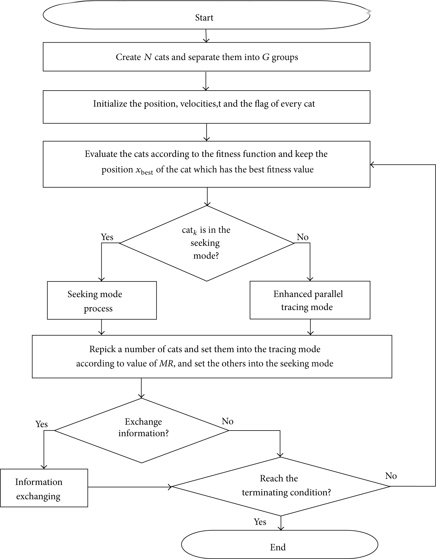
The flowchart of EPCSO algorithm.
A brief review of EPCSO algorithm is given as follows.
Step 1.
Create N cats, randomly classify the cats into the M-dimensional solution space within the limited ranges of the initial value, and randomly split them into G groups. Generate the velocities for each dimension of each cat and set the motion flags that define which mode the cat belongs to be according to the user predefined value of MR, where
Step 2.
By taking the cats’ coordinates into fitness function to evaluate the fitness values, respectively, record the best coordinate and the fitness value of the cat which has the better fitness value calculated so far.
Step 3.
Move the cats by the seeking mode process or the tracing mode process. If the cat is assigned into seeking mode, it takes (4) and (5). Otherwise, it takes (6)–(9) according to the statues of the motion flag.
Step 4.
Reset the motion flag for all cats. Repick and separate
Step 5.
Check whether the number of iterations reaches a predefined iteration number or not. If it is satisfied, run the information exchanging process.
Step 6.
Check whether the termination criteria are satisfied. If the answer is positive, output the coordinate, which represents the best solution found in the whole process and terminate the program. Otherwise, go back to Step 2 and repeat the process.
2.2.1. The Seeking Mode Process
Tsai et al. define 4 essential parameters in the seeking mode process, that is, the seeking memory pool (SMP), the seeking range of the selected dimension (SRD), the counts of dimension to change (CDC), and the self-position considering (SPC). These parameters affect the searching ability, directly, because they are related to the quantity of the changes caused to the cats. The seeking mode process is briefly reviewed as follows.
Step 1.
Generate SMP copies of the present position of cat. If SPC value is true, then store the present position as one of the candidates.
Step 2.
For each copy cat, according to CDC, randomly plus or minus SRD percent values and replace the old ones:

Here rand is a random variable in the range
Step 3.
Calculate the fitness values (FS) of all candidate points, respectively.
Step 4.
If all FS are not exactly equal, calculate the selecting probability
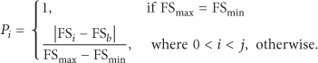
If the goal of the optimization process is to find the minimum solution of the fitness function, let
Step 5.
Pick the coordinate from the candidate points to move to base on the probability.
2.2.2. The Parallel Tracing Mode Process
Once a cat runs into tracing mode, it migrates according to its’ own velocities corresponding to every dimension. The parallel tracing mode process can be depicted as follows.
Step 1.
Generate two sets of the velocities for every dimension

where M denotes the dimension of the solution space,

where s is the index of the velocity set.
Step 2.
Take one velocity set to update the original velocity
Then update the position

Calculate its fitness value for later use. Accumulate the FS values contributed by the column factors and take the most adaptive factors to compose the latest velocity.
Step 3.
Move the present
2.2.3. The Information Exchanging Process
This process aims at exchanging subpopulation information and forming the cooperation structure between different groups. There is a factor ECH to monitor the condition of each subpopulation. After ECH number iterations, these subpopulations exchange information once. Four steps of the exchanging process are showed as follows.
Step 1.
Pick up a group of subpopulations sequentially and sort these cats according to their FS values.
Step 2.
Randomly select a local best solution from an unrepeatable group.
Step 3.
Replace the position of the worst of cat whose FS value is the worst with the local best solution cat position.
Step 4.
Repeatedly perform Step 1 to
3. Network Model Deployment
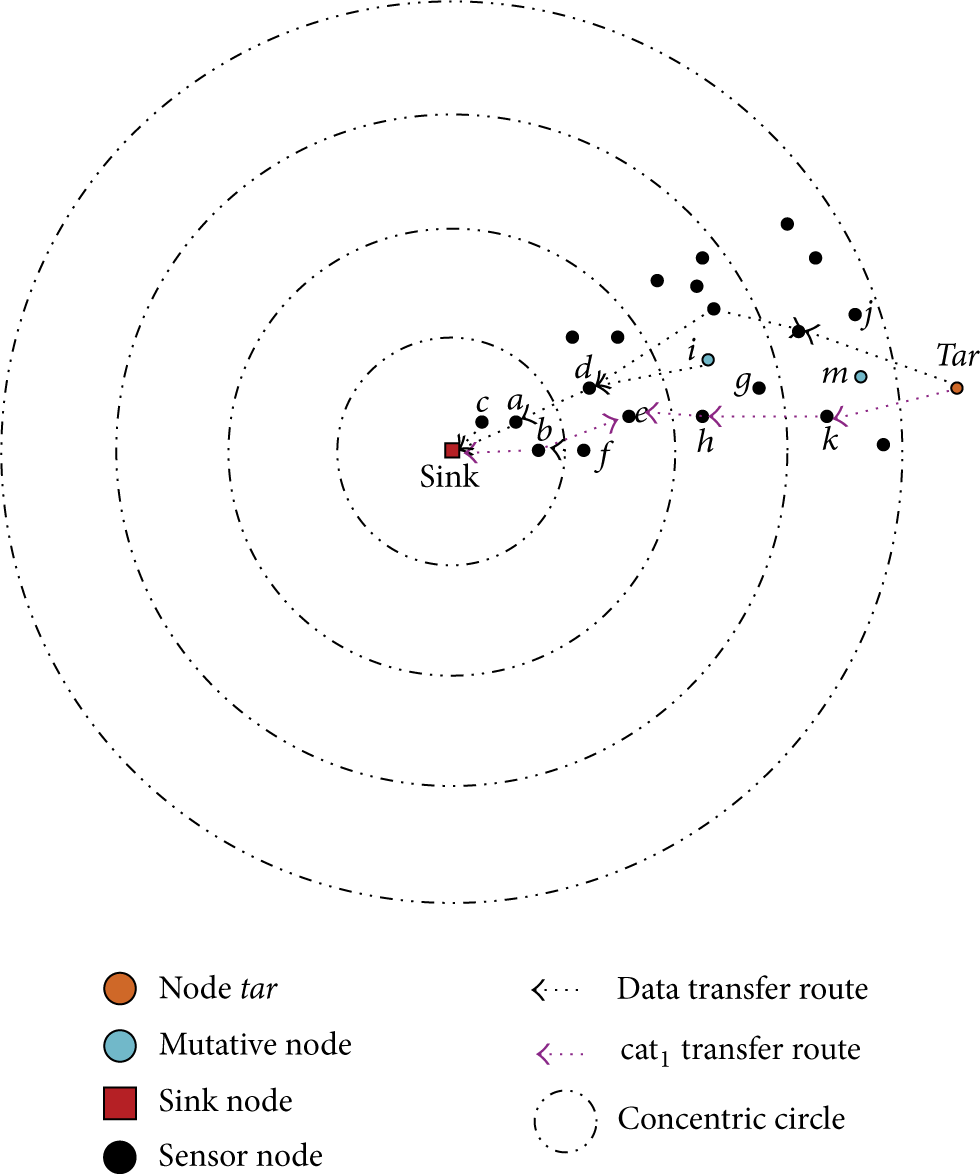
In this paper, we consider two-dimensional static flat environment and assume each node equipped with the same fixed transmission range. The network region is a circle with radius 350. It would be much easier and cheaper than predefined position deployment. However, for the sake of diminishing the critical nodes workload and then prolonging the whole network lifetime, we propose a scheme for the sensor deployment. The closer to the sink node results in the more power consumption is a definite fact in deploying sensor nodes. The reason is that the nodes closer to the sink node are much frequently treated as the delay nodes. To overcome the power consumption problem, it is necessary to increase the number of nodes in the regions near to the sink node. Answering to the problem mentioned above, we propose a scheme to deploy the sensor nodes by calculating the required density of the sensor nodes. To deploy sensor nodes in a two-dimensional field, we divide the field into 7 concentric circles, 8 sectors, and 56 subboxes as shown in Figure 2.

A quarter of network structure.
There are 2,688 sensor nodes deployed in this field. The outer layer is defined as sectors on the 7th concentric circle; and the inner layer is defined as sectors numbered as 1 to 6 on the 1st concentric circle. For the outer layer concentric circles, each sector is assigned 48 sensor nodes scattered randomly to the field. Based on this condition, the same amount of sensor nodes is assigned to all sectors. This result in the coverage intensity is increased in the inner layer sectors. Therefore, the payload of WSN in the inner layer sectors can be shared with more optional paths. The power consumption is now with larger chance to be balanced automatically by deploying sensor nodes with higher density in the inner layer sectors. Furthermore, the possibility of network paralyzing caused by disabled internal nodes is reduced. In addition, the lifetime of the WSN is also extended. For a fixed amount of sensor nodes, the larger the measure of area is, the lower the coverage intensity is. To ensure the WSN is functional, the network coverage intensity must be above a certain threshold. Hence, in our deployment strategy, the minimum amount of sensor deployed in a sector is calculated based on the sector located on the outer layer. This deployment strategy is easy to operate. And the result is capable of achieving high coverage intensity. The proof of high coverage intensity is given as follows.
Proof.
For the reason that the shape of each sector is not a circle, we cannot directly apply the minimum number of nodes theory to the sector area. Thus, we use the derivation method to verify the high coverage intensity. First, we calculate the coverage intensity value of an area covered by 48 sensor nodes. According to reverse deduction, the whole network minimum coverage intensity can be found.
Only one subset exists in the WSN,
where a is the area of circle with radius 350, which covers the whole region, and r denotes the size of sensing area of one node. It is known that the outer layer sector such as number 49, which is covered by 48 sensor nodes, satisfies the minimum full coverage condition. The same coverage intensity can be treated as the criterion for defining the number of sensor nodes used in other sectors to achieve the same coverage condition. The number of sensor nodes can be figured out by the equivalent proportional relationship. The area ratio of sector 49 to the whole field is In (10), given q, we get Finally, taking q, k, S into (10), we get


The area of a sector located in the outer layer such as sector 49 is larger than any sectors in the other layers. Hence, the coverage intensity of the most outer layer concentric is definitely smaller than the inner layer concentric sectors. In order to ensure a good data forwarding quality, the whole network coverage intensity is designed to be greater than 0.99. Based on the criteria mentioned above, the overview of the WSN based on our proposed deployment scheme is shown in Figure 3.
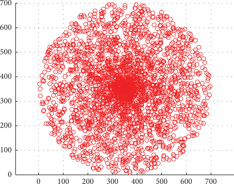
Network node deployment result.
4. Using EPCSO Method to Solve the Routing Problem in WSN
In the wireless sensor network, we need to build routing path for every sensor node. The routing path is different in the number of relay nodes for each concentric circle node. However, the EPCSO originally is not a method used in finding paths for the WSN. Its first application is designed for the aircraft schedule recovering. Thus, we have to partially modify EPCSO before employing it to solve the routing problem in WSN. The modifications we made for EPCSO in this paper are listed as follows: (1) The representation of the artificial agent is modified from the coordinate to a set. (2) A newly defined cluster flag is added into the basic component of the artificial agent. (3) The newly designed fitness function is custom-made for the WSN routing problem.
Assume that the transmission range of a single sensor node is 50. Thus, the nodes located in the sectors in the 5th concentric circles need four relay nodes to transmit their package to the sink node. We use node tar as an example to explain how to use EPCSO to solve the routing problem. The modified EPCSO and the whole processes are explained as follows.
4.1. Initialization
In the initialization process, some parameters and constants are required to be defined before the whole process starts. In the original EPCSO, the artificial agent (the cat) is composed of the coordinate representing its position in the solution space. In our design, the artificial agent is composed by a set of sensor nodes. The sensor nodes in one set are from different layers and should be capable of forming at least one complete path from the most outer layer back to the sink node. For each cat, the set is defined by

where i is the identity index of the cat and l is the identifier of the concentric circle (the layer). In this application, the population size is set to 16. There are three backup sensor nodes located in the same layer in every cat. As shown in Figure 4, sensor node tar in the given example is located on the 5th layer.
One of the initialized cats for node tar.
In this case, one of the initialization results of node tar can be described by

As given in (13),

The velocity is corresponding to the composition of cat. For example,
where l stands for the numerical value of concentric circles and
4.2. Custom-Made Fitness Function
The fitness function (also called the object function or the evaluation function) plays the principal role in the whole process. A well-designed fitness function should be capable of representing the input solution's behavior in the solution space.
To utilize the modified EPCSO in finding the balanced path for the WSN, a fitness function is designed specifically for this goal. Our proposed fitness function can be described by
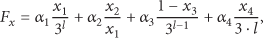
where
Path Number (
Total Power Consumption (
Relay Number (
Usage Number (
The fitness function can be decomposed into 4 parts, that is, the path ratio, the average power consumption, the relay ratio, and the usage rate. The detailed description is listed as follows.
Path Ratio. The path ratio is defined by (17); it stands for the ratio of the found path numbers to the ideal path in the cat:

where Pathratio represents the path ratio, l is the position circles minus one, and the ideal path number is known as
Average Power. The average power is defined by (18). Avepower calculates the power consumption on average over all paths carried by the cat:

Relay Ratio. The relay ratio is defined by (19). It is known that, in the ideal case, the total relay number is

Usage Rate. The usage rate is defined by (20). It stands for the ratio of the usable nodes to all nodes collected by the cat. In the ideal case, all nodes carried by a cat should be useable; that is, the usage rate is equal to 1:

The fitness function is employed in the EPCSO process to evaluate the fitness of the cats and is the gauge to find the global near-the-best solution (denoted by
4.3. An Example Is Given as Follows
Assume the target node tar is located in the 5th layer as shown in Figure 4; the parameter l is 4. For cat1, we have
4.4. Seeking Mode Process
Suppose cat1 is assigned to move by the seeking mode process; j copies of

Assume
An example of

The result of
4.5. Tracing Mode Process
In the tracing mode process, the cat's velocity should be updated, and the cat will be moved based on its velocity produced by the Taguchi method. The velocity is produced based on
The

5. Experiment and Experimental Result
The experimental result is produced by our proposed routing method based on the minimum-number-node theory and the modified EPCSO. As mentioned above, 2,688 nodes are deployed in a 2D field within a 350-radius circle. The circle is divided into 7 concentric circles and each of the concentric circles contains the same number of sensor nodes, that is, 384 nodes. The experimental result of the total power consumption produced by our proposed method is compared with LDACO [10], AODV [6], and LDCSO [7] in Table 2. In our simulation, we only count the routing power consumption. The routing path is from one node that senses an event to the sink. In the first column, “all” stands for the power consumption caused by all sensor nodes deployed in the environment, “one” means the power consumption caused by all sensor nodes located in the most inner layer, “two” is the power consumption caused by the sensor nodes located in the 2nd layer, and “seven” is the power consumption caused by the sensor nodes located in the most outer layer. The experimental result indicates that the whole power consumption is
The results of four algorithms.

6. Conclusion
In this paper, we propose a strategy for deploying the sensor nodes by considering the coverage of WSN based on the minimum-number-node theory. Furthermore, we utilize EPCSO to design a routing algorithm for providing the balanced routing paths. Three modifications are made for the EPCSO algorithm to make it suitable for finding routing paths for WSN. Our design balances the power consumption between the forwarding distance and the energy saving for all nodes in the whole WSN. Our deployment strategy is easy to use in different WSN applications. Furthermore, the problem of which the inner layer nodes usually are out of battery is solved because our deployment method with EPCSO finding transmission paths keeps the sensor nodes in the inner layer alive and the nodes in the most outer layer are firstly out of battery.
The experimental result indicates that our proposed method could partially balance the power consumption between the inner layer and the outer layer. The total power consumption of our proposed method is the lowest among other algorithms. The simulation results indicate that our proposed method reduces more than 35% power consumption on average.
Footnotes
Conflict of Interests
The authors declare that there is no conflict of interests regarding the publication of this paper.