Delay Minimization Topology Control in Planetary Surface Network: An Autonomous Systems Approach

Abstract

This paper investigates the topology control problem in the planetary surface network (PSN) of Interplanetary Internet (IPN) using an autonomous system (AS) approach. We propose a delay minimization topology control (DMTC) algorithm to achieve low time delay and strong connectivity in the planetary surface network. Compared with the most existing approaches where either the purely centralized or the purely distributed control method is adopted, the proposed algorithm is a hybrid control method. In order to reduce the cost of control, the control message exchange is constrained among neighboring AS networks. We prove that the proposed algorithm could achieve logical k-connectivity on the condition that the original physical topology is k-connectivity. Simulation results validate the theoretic analysis and effectiveness of the DMTC algorithm.

1. Introduction

The Interplanetary Internet (IPN) was proposed to satisfy the demands of deep space communications early in this century. As proposed in [1, 2], the IPN includes a backbone network, external networks, and planetary networks (PNs). A PN is composed of an orbiter network (ON) and a planetary surface network (PSN). The former is composed of orbiters circling the planets and provides a relay service between the surface network and the backbone network [3, 4]. The latter is composed of landers, rovers, astronauts, and sensors from different countries or space missions [5, 6]. Nodes in the planetary surface network autonomously connect to each other in order to perform collaborative tasks. Unlike wireless sensor network (WSN) on the earth, the PSN has distinguishing characteristics [7]. The scale of the PSN is large. Communication abilities of nodes in the PSN are usually stronger. Nodes in the PSN have a wide and uneven distribution. Some links among them are short and some are extremely long. Excessive use of these long-distance links data not only brings additional delay but also reduces operation efficiency. What is more, long links usually mean more energy will be consumed. Consequently, how to make an efficient and reliable topology control is challenging.

Existing works about network topology control mainly focus on maintaining a specified topology and achieve a set of network-wide objectives such as reducing energy consumption, guaranteeing the robustness, increasing the network capacity, and reducing end-to-end delay, for example, [8–16]. But, in most studies, either the purely centralized or the purely distributed control method is adopted. Centralized algorithms rely on a central entity which knows the conditions of all the nodes in order to calculate the optimal topology [17–19]. However, these algorithms are not suitable for large scale network such as PSN where excessive amounts of control messages need to be collected by one central entity. Control information in the PSN is costly for long distance and too many hops. On the other hand, in distributed algorithms, each node collects the information from its neighboring nodes and autonomously computes which link should be preserved [19–21]. Consider that the information each node obtains is limited; the final topology usually cannot achieve global optimization for large scale networks. Thus, it is important to develop a special topology control algorithm for the PSN.

Instead of using long links, nodes in the PSN should collaboratively determine which links will be used and define the network topology though forming proper neighbor relations. That is, topology control algorithms of the PSN actually remove unnecessary long links. As a result, the network topology is susceptible to unpredictable events such as hardware failures in such a harsh environment. Therefore, to design robust topology control algorithms, k-connectivity of the network is considered, where a k-connected network is $k-1$ fault-tolerant; that is, the failure of less than $k-1$ nodes will not disconnect the whole network.

In this paper, we study the topology control problem in the PSN using an autonomous system (AS) approach. An AS network is a collection of nodes with similar properties, for example, nodes distributed in the same region. The reasons for using the AS approach are twofold. Firstly, the complex PSN is decoupled into a series of small AS networks, and centralized method can be used in each AS to ensure strong connectivity. Secondly, distributed method is used among AS networks; thus the topology control message exchange can be constrained among neighboring AS networks. We propose a delay minimization topology control (DMTC) algorithm using such a hybrid approach. DMTC preserves k-connectivity and is min-max delay optimal. The min-max criterion tries to minimize the maximum end-to-end delay between any pair of nodes in the network [22]. Briefly, the DMTC algorithm consists of three phases: (i) nodes in the PSN autonomously form AS networks and elect AS cores; (ii) with the topology information gathered from the members of its AS network, each AS core minimizes the maximum link delay used by all the nodes and guarantees strong connectivity using a centralized method; (iii) each AS core selects a set of border nodes, shares topology information with neighboring AS cores, and computes low time delay links between neighboring AS networks using a distributed method. The main contributions of this paper are summarized as follows:

• (1)

An AS network model of PSN is proposed. The large scale and complex PSN is decoupled into small AS networks with similar nodes to achieve strong connectivity with low cost control messages.

(2)

A delay minimization topology control (DMTC) algorithm is proposed to achieve low time delay. It is a hybrid algorithm within an AS network and among neighboring AS networks.

(3)

The strong connectivity of DMTC algorithm proved that the algorithm could achieve logical k-connectivity on the condition that the original physical topology is k-connectivity.

The rest of this paper is organized as follows. In Section 2, we define the network model and provide some definitions. In Section 3, we propose an AS based algorithm DMTC to achieve low time delay and strong connectivity. Then, the validity of DMTC is proved in Section 4, and the message complexity of our algorithm is analyzed in Section 5. In Section 6, simulation results and discussion are presented. Finally, we make conclusion in Section 7.

2. Network Model

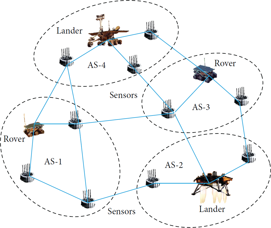
In this section, the network model of AS network is defined. As presented above, the PSN is a self-organizing system constituted by various nodes. For example, as demonstrated in Figure 1, the Mars PSN is a part of the IPN. Nodes in the PSN have a wide and uneven distribution. They work in different areas with either mobile (e.g., rovers) or static (e.g., sensors) statuses. If we apply a unified strategy to manage the whole PSN, it will induce low efficiency and even cannot maintain the normal operation of the network with too much control information. So, as shown in Figure 2, we divide the PSN into a series of AS networks according to the property of the nodes. Each AS network can adopt independent topology control strategy to achieve strong connectivity. And the control message exchange is constrained among neighboring AS networks to reduce the cost of control.

Figure 1

The PSN is a part of the IPN and is a self-organizing system constituted by various nodes.

Figure 2

The whole PSN is divided into a series of AS networks according to the property of the nodes.

Considering that the properties of nodes in the PSN are similar except few nodes, we assume that all the nodes are homogeneous. They have the same maximal transmission range $R_{\mathrm{m}\mathrm{a}\mathrm{x}}$ . Let the PSN network topology be represented by undirected simple graph $G=\left(V,E\right)$ , where $V=\left\{u_{\mathrm{1}},u_{\mathrm{2}},\dots ,u_n\right\}$ is the set of nodes (or, equivalently, vertices) and $E=\left\{\left(u_i,u_j\right)\hspace{0.17em}|\hspace{0.17em}\left(u_i,u_j\in V\right)\wedge \left(r\left(u_i,u_j\right)\le R_{\mathrm{m}\mathrm{a}\mathrm{x}}\right)\right\}$ is the set of links (edges). $r\left(u_i,u_j\right)$ is the distance between nodes $u_i$ and $u_j$ . Each node is assigned a unique identifier (ID) according to its property, such as MAC address.

We assume that G is a general graph; that is, if $\left(u,v\right)\in E$ , u and v can exchange information with each other. We also assume that the link is symmetric and obstacle-free, and each node is able to obtain its location by some means (e.g., celestial navigation [23], initial navigation [24], and vision navigation [25]). We then define several graphs related terms in the following, which will be used in both algorithms and proofs. For all definitions, we refer to graph $G=\left(V,E\right)$ and subgraphs $G_i=\left(V_i,E_i\right)$ and $G_j=\left(V_j,E_j\right)$ .

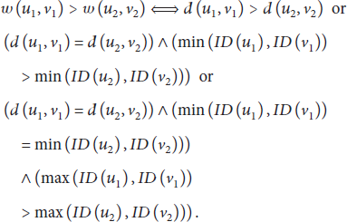
Definition 1 (weight function).

For edge $e=\left(u,v\right)$ , the weight function is $w\left(u,v\right)=\left(d\left(u,v\right),\mathrm{m}\mathrm{i}\mathrm{n}\left(ID\left(u\right),ID\left(v\right)\right),\mathrm{m}\mathrm{a}\mathrm{x}\left(ID\left(u\right),ID\left(v\right)\right)\right)$ , where $d\left(u,v\right)$ is the time delay between u and v when exchanging information. Given $\left(u_{\mathrm{1}},v_{\mathrm{1}}\right),\left(u_{\mathrm{2}},v_{\mathrm{2}}\right)\in E$ , the relationship between $w\left(u_{\mathrm{1}},v_{\mathrm{1}}\right)$ and $w\left(u_{\mathrm{2}},v_{\mathrm{2}}\right)$ is given as

$$\begin{array}{cc}& w\left(u_{\mathrm{1}},v_{\mathrm{1}}\right)>w\left(u_{\mathrm{2}},v_{\mathrm{2}}\right)⟺d\left(u_{\mathrm{1}},v_{\mathrm{1}}\right)>d\left(u_{\mathrm{2}},v_{\mathrm{2}}\right)\hspace{0.17em}\hspace{0.17em}\text{or}\\ \left(d\left(u_{\mathrm{1}},v_{\mathrm{1}}\right)=d\left(u_{\mathrm{2}},v_{\mathrm{2}}\right)\right)\wedge \left(\mathrm{m}\mathrm{i}\mathrm{n}\left(ID\left(u_{\mathrm{1}}\right),ID\left(v_{\mathrm{1}}\right)\right)>\mathrm{m}\mathrm{i}\mathrm{n}\left(ID\left(u_{\mathrm{2}}\right),ID\left(v_{\mathrm{2}}\right)\right)\right)\hspace{0.17em}\hspace{0.17em}\text{or}\\ \left(d\left(u_{\mathrm{1}},v_{\mathrm{1}}\right)=d\left(u_{\mathrm{2}},v_{\mathrm{2}}\right)\right)\wedge \left(\mathrm{m}\mathrm{i}\mathrm{n}\left(ID\left(u_{\mathrm{1}}\right),ID\left(v_{\mathrm{1}}\right)\right)=\mathrm{m}\mathrm{i}\mathrm{n}\left(ID\left(u_{\mathrm{2}}\right),ID\left(v_{\mathrm{2}}\right)\right)\right)\wedge \left(\mathrm{m}\mathrm{a}\mathrm{x}\left(ID\left(u_{\mathrm{1}}\right),ID\left(v_{\mathrm{1}}\right)\right)>\mathrm{m}\mathrm{a}\mathrm{x}\left(ID\left(u_{\mathrm{2}}\right),ID\left(v_{\mathrm{2}}\right)\right)\right).\end{array}$$

(1)

It is obvious that edges with the same vertices have equivalent weights. However, edges with different end-vertices have different weights.

Definition 2 (k-connected).

In graph (topology) G, node u is said to be connected to node v, if there exists path $p=\overline{u{x}_{\mathrm{1}}{x}_{\mathrm{2}}\cdots x_{m-\mathrm{1}}{x}_{m}v}$ , where $x_i\in V$ and $\left(u,x_{\mathrm{1}}\right),\left(x_i,x_j\right),\left(x_m,v\right)\in E$ . And, for any $u,v\in V$ , if there exist at least k disjoint paths between them. Graph G is k-connected and denoted by $CON\left(G,k\right)$ . If G is k-connected, it follows that there does not exist a set of $k-1$ vertices, whose removal will partition G into two or more connected components.

Definition 3 (neighboring k-connected subgraphs).

For two disjoint subgraphs $G_i$ and $G_j$ of G, if $\exists u\in V_i,v\in V_j$ , and $\exists \left(u,v\right)\in E$ , $G_i$ and $G_j$ are neighboring subgraphs, denoted by $NB{R}_G\left(G_i,G_j\right)$ . If $CON\left(G_i,k\right)\wedge CON\left(G_j,k\right)$ and $\exists \left(u_{\mathrm{1}},v_{\mathrm{1}}\right),\dots ,\left(u_k,v_k\right)\in E$ , where $u_{\mathrm{1}},\dots ,u_k\in V_i$ and $v_{\mathrm{1}},\dots ,v_k\in V_j$ , $G_i$ and $G_j$ are neighboring k-connected subgraphs, denoted by $NB{R}_G\left(G_i,G_j,k\right)$ .

Definition 4 (multihop k-connected subgraphs).

Let $G_{\mathrm{1}},G_{\mathrm{2}},\dots ,G_n$ be partitioning of G. If $\exists G_l$ subject to $NB{R}_G\left(G_i,G_l,k\right)\wedge NB{R}_G\left(G_l,G_j,k\right)$ , $G_i$ and $G_j$ are multihop k-connected subgraphs, denoted by $MCO{N}_G\left(G_i,G_j,k\right)$ .

3. Algorithms for Topology Control

Recall from Introduction that the design aims of the DMTC algorithm are twofold, (1) to provide min-max delay optimal through an AS approach and (2) to achieve strong connectivity in the resulting network. The DMTC algorithm does not require the global topology of the PSN network to be known by any entity. On the contrary, DMTC relies on AS networks where nodes autonomously form groups and select a core for each AS network. It is a hybrid of centralized algorithm and distributed algorithm. A centralized topology control algorithm is applied to each AS network to achieve the desired connectivity within the AS, while the desired connectivity between adjacent AS networks is achieved via localized information sharing between adjacent AS cores. The following subsections detail the three phases of the DMTC algorithm.

3.1. Phase 1: AS Network Formation

The main function of Phase 1 is to select a minimal number of nodes as cores that dominate the AS networks by using only 1-hop transmission. And these cores will take the main responsibility for the subsequent two phases.

Step 1 (broadcasting hello messages).

When starting up, each node broadcasts hello messages periodically in order to let them discover each other in the surrounding area. A hello message is of the form $\left(NodeID,Location,CoreID,Degree,Delay\right)$ . The explanation of each field is as follows: $(1)\hspace{0.17em}\hspace{0.17em}NodeID$ : the unique ID of each node; $(2)\hspace{0.17em}\hspace{0.17em}Location$ : the location of each node; $(3)\hspace{0.17em}\hspace{0.17em}CoreID$ : the ID of the core with which the sending node is currently associated; if the sending node does not associate with any core, it is zero; note that a core node uses its own ID for this field; $(4)\hspace{0.17em}\hspace{0.17em}Degree$ : the degree of connectivity (the number of neighbors); $(5)\hspace{0.17em}\hspace{0.17em}Delay$ : time delay to each neighbor when exchanging information. It may contain processing, transmission, and propagation delay in practice. In order to facilitate the analysis, we only consider propagation delay in this paper.

Step 2 (core selection process).

The core selection process of each node begins after it has broadcasted hello messages for a certain waiting time. The waiting time should be long enough to allow this node to receive at least one hello message from every immediate neighbor. In this process, every node will decide whether it is suitable as a core of an AS or become a member of an AS by checking for its local optimality. Each node computes its own height from its current states. The height metric should be chosen to suit the design goals of the PSN topology control algorithm. As a result, we use $\left(Delay,Degree,NodeID\right)$ as the height metric. $NodeID$ is included in the metric calculation to break ties. The height function is $height\left(u\right)=\left(h\left(u\right),ID\left(u\right)\right)$ . In order to balance the factor of $Delay$ and $Degree$ , we formulate $h\left(u\right)$ as

$$\begin{array}{cc}& h\left(u\right)=f\left(Degree\left(u\right),Delay\left(u,v_i\right),\alpha \right),\end{array}$$

(2)

where $f\left(·\right)$ denotes the balance function and α is the balance factor. The relationship between $hight\left(u\right)$ and $hight\left(v\right)$ is given by

$$\begin{array}{cc}& hight\left(u\right)>hight\left(v\right)⟺h\left(u\right)>h\left(v\right)\hspace{0.17em}\hspace{0.17em}\text{or}\\ \left(h\left(u\right)=h\left(v\right)\right)\wedge \left(NodeID\left(u\right)>NodeID\left(v\right)\right).\end{array}$$

(3)

Then, if a node has the highest height among its neighbors, it is considered as a local optimal node and should serve as a core. After this process, the first batch of cores is selected, and all consequent hello messages will be changed accordingly.

Step 3 (supplement of cores).

After Step 2, each node checks if there are cores in the range $R_{\mathrm{m}\mathrm{a}\mathrm{x}}$ . If cores exist, it will regard the core that has the least $Delay$ between them as its parent. That is, this node will be the member of the AS dominated by its parent core. Then nodes update the $CoreID$ in their hello messages with their parent cores' ID. Note that a core node uses its own ID for this field. After that, nodes whose $CoreID$ are zero without parent calculate their height functions. And the node that has the highest height among its neighbors without parent in the range $R_{\mathrm{m}\mathrm{a}\mathrm{x}}$ should serve as a core.

Step 4 (optimization and maintenance process).

Considering nodes' mobility, and in order to keep the number of cores as low as possible, if a core detects there are other cores in the range $R_{\mathrm{m}\mathrm{a}\mathrm{x}}$ (from the hello process), it will check whether it has the highest height among these cores. If not, it will turn into a member of the highest height core, and its member nodes will turn into nodes without parent. If there exist nodes without parent in the PSN, process will turn to Step 3. Finally, there are only two kinds of nodes: cores and members. And this optimization and maintenance process will keep monitoring the PSN. For instance, if a new node is added to the PSN, the process will take this node as a node without parent and turn to Step 3.

3.2. Phase 2: Intra-AS Topology Control

In this phase, we present a centralized algorithm for intra-AS network. Each core will calculate the links for all of the members of its AS such that the resulting topology of the AS meets the given topology constraint (min-max delay and k-connectivity). The intra-AS topology control algorithm is described in Algorithm 1, where G represents the PSN, and let $G_{\mathrm{1}},G_{\mathrm{2}},\dots ,G_n$ (AS) be partitioning of G.

Algorithm 1: Intra-AS topology control.

Input: (at AS $G_s=(V_s,E_s)$ )

 k (required connectivity)

Output:

  $G_k=(V_k,E_k)$

Begin:

  $V_k\leftarrow V_s$ , $E_k\leftarrow \mathrm{\varnothing }$

 Sort all edges in $E_s$ in ascending order of weight (as defined in Definition 1)

 for all edge $(u_i,v_i)$ in the order do

  if   $u_i$ is not k-connected to $v_i$   then

    $E_k\leftarrow E_k\cup (u_i,v_i)$

  end if

 end for

 for all edge $(u_j,v_j)$ of $E_k$ in the descending order do

  if   $u_j$ is still k-connected to $v_j$ with the disconnection of edge $(u_j,v_j)$   then

    $$E_k\leftarrow E_k-(u_j,v_j)$$

  end if

 end for

Return   $G_k$

For each AS, Algorithm 1 ensures that $G_k$ preserve the k-connectivity of $G_s$ ; that is, $CON\left(G_s,k\right)\Rightarrow CON\left(G_k,k\right)$ . And the maximum end-to-end delay among all edges in the AS network is minimized by Algorithm 1; that is, let $D_{\mathrm{m}\mathrm{a}\mathrm{x}}\left(G_k\right)$ be the maximum delay of all edges in the AS minimized by Algorithm 1, and let $S_k\left(G_s\right)$ be the set of all kinds of k-connected subgraphs of $G_s$ with the same vertices $V_s$ ; then we have $D_{\mathrm{m}\mathrm{a}\mathrm{x}}\left(G_k\right)=\mathrm{m}\mathrm{i}\mathrm{n}\left\{D_{\mathrm{m}\mathrm{a}\mathrm{x}}\left(G_i\right)\hspace{0.17em}|\hspace{0.17em}{G}_i\in S_k\left(G_s\right)\right\}$ . The correctness of Algorithm 1 is provided in Section 4.

3.3. Phase 3: Inter-AS Topology Control

In this phase, connectivity between adjacent AS networks is considered. In order to allow adjacent AS networks to discover each other, every node continues broadcasting hello message $\left(NodeID,Location,CoreID,Degree,Delay\right)$ as in Phase 1 periodically. When node u receives a hello message from node v that belongs to a different AS (e.g., they have different $CoreID$ ), u will place v's information in its border list. Then this border list is reported to the node's parent core. With these border lists, we present a distributed algorithm for inter-AS. This algorithm is described in Algorithm 2, where G represents the PSN, and let $G_{\mathrm{1}},G_{\mathrm{2}},\dots ,G_n$ (AS) be partitioning of G.

Algorithm 2: Inter-AS topology control.

Input: (at AS $G_k=(V_k,E_k)$ )

 k (required connectivity)

Output:

 Links for all nodes in $G_k$ 's border list.

Begin:

  $G_{ki}=(V_{ki},E_{ki})$ , $V_{ki}\leftarrow V_k$ , $E_{ki}\leftarrow \mathrm{\varnothing }$

 for  all $G_i$ subject to ${NBR}_G(G_k,G_i)$   do

   $V^{\prime }\leftarrow \{v\hspace{0.17em}|\hspace{0.17em}(v\in G_i)\wedge (v\hspace{0.17em}\hspace{0.17em}\mathrm{i}\mathrm{s}\hspace{0.17em}\hspace{0.17em}\mathrm{a}\mathrm{d}\mathrm{j}\mathrm{a}\mathrm{c}\mathrm{e}\mathrm{n}\mathrm{t}\hspace{0.17em}\hspace{0.17em}\mathrm{t}\mathrm{o}\hspace{0.17em}\hspace{0.17em}{G}_k)\}$

   $V_{ki}\leftarrow V_{ki}\cup V^{\prime }$

   $E_{ki}\leftarrow \{(u,v)\hspace{0.17em}|\hspace{0.17em}(u\in V_k)\wedge (v\in V^{\prime })\wedge (r(u,v)\le R_{\mathrm{m}\mathrm{a}\mathrm{x}})\}$

   $M\leftarrow \mathrm{\varnothing }$

   $E_a$ ← sort all edges in $E_{ki}$ in ascending order of weight (as defined in Definition 1)

   $k_m\leftarrow \left|MaxMatching(G_{ki})\right|$

  %   $\left|MaxMatching(G_{ki})\right|$ is the number of edges in $MaxMatching(G_{ki})$

  if   $k_m\ge k$   then

   for  all edges $e_t=(u_t,v_t)\in E_a$ in the order  do

    Find the smallest t, subject to $\left|M\right|\ge k$ , where $M\leftarrow MaxMatching(G_t=(V_{ki},E_a(t)))$ , and $\left|M\right|$ is the number of

    edges in M, $E_a\left(t\right)=\{e_{\mathrm{1}},\dots ,e_t\}$

   end for

    $D_{IA}(G_k,G_i)\leftarrow \left|e_t\right|$ , where $\left|e_t\right|$ is the weight of $e_t$

    $L(G_k,G_i)\leftarrow M$

  else

   for  all edges $e_t=(u_t,v_t)\in E_a$ in the order  do

    Find the smallest t, subject to $\left|M\right|\ge k_{\mathrm{2}}$ , and $M\leftarrow MaxMatching(G_t=(V_{ki},E_a(t)))$

   end for

    $D_{IA}(G_k,G_i)\leftarrow \mathrm{\infty }$

    $L(G_k,G_i)\leftarrow M$

  end if

  Send $D_{IA}(G_k,G_i)$ to neighbor AS

 end for

 Collect $D_{IA}$ from neighboring AS

  $LIST\leftarrow \mathrm{\varnothing }$

 for  all $G_p$ subject to ${NBR}_G(G_k,G_p)$   do

  if  there does not exist $G_q$ subject to

    ${NBR}_G(G_k,G_q)\wedge {NBR}_G(G_k,G_p)\wedge$

    $(D_{IA}(G_k,G_q)<D_{IA}(G_k,G_p))\wedge$   then

    $(D_{IA}(G_p,G_q)<D_{IA}(G_k,G_p))$

      $LIST\leftarrow LIST\cup L(G_k,G_i)$

  end if

 end for

Return   $LIST$

In this algorithm, the core of AS A checks whether there exist k disjoint links from this AS to each adjacent AS B. That is accomplished by applying an algorithm ( $MaxMatching$ ) [26] that computes a matching of maximum cardinality in a bipartite graph defined by the nodes in respective AS networks and the edges with one vertex in each AS. If k does not exceed the size of maximum cardinality matching, the core of AS A selects k disjoint links that meet the min-max delay optimal. When there do not exist k disjoint links between A and B (only $k_m$ disjoint links), the core preserves the $k_m$ -connectivity between these two AS networks and minimizes the maximum delay between them. Note that this connectivity preservation ( $k_m$ -connectivity) cannot guarantee k-connectivity between AS A and B. However, global k-connectivity can be guaranteed after Phase 3 is completed when connectivity with other neighboring AS networks is already established. This will be proved in Section 4.

Parameter $D_{IA}\left(G_{\mathrm{1}},G_{\mathrm{2}}\right)$ in Algorithm 2 is used to perform an optimization which removes unnecessary links between certain adjacent AS networks, while preserving the connectivity of the resulting topology. $D_{IA}\left(G_{\mathrm{1}},G_{\mathrm{2}}\right)$ is the maximum delay of the selected k links. However, when the number $k_m$ of disjoint links between two adjacent AS networks is less than k, $D_{IA}\left(G_{\mathrm{1}},G_{\mathrm{2}}\right)$ is ∞. Then, AS A will not connect to neighboring AS B directly if it observes that there exists another AS C, where C is also a neighbor of B, and both $D_{IA}\left(G_A,G_C\right)$ and $D_{IA}\left(G_B,G_C\right)$ are less than $D_{IA}\left(G_A,G_B\right)$ .

After Phase 3 is completed, each node is assigned a link list, and nodes connect to each other according to these lists. This topology will be maintained by every node with hello message periodically and always preserve the objective connectivity of the network.

4. Proof of Strong Connectivity

In this section, we prove the strong connectivity of Algorithms 1 and 2 [27]. The results are given as the following theorems.

4.1. Strong Connectivity of Algorithm 1

Theorem 5.

Algorithm 1 can preserve k-connectivity of AS $G_s$ ; that is, $CON\left(G_s,k\right)\Rightarrow CON\left(G_k,k\right)$ . And the maximum delay among all nodes in the network is minimized by Algorithm 1.

Before proving the correctness of Theorem 5, two lemmas are first provided. Let $p=\overline{u{x}_{\mathrm{1}}{x}_{\mathrm{2}}\cdots x_{m-\mathrm{1}}{x}_{m}v}$ be the path from node u to v (as defined in Definition 2). Let the maximal set of disjoint paths from node u to v in graph $G_s$ be represented by $P_{u,v}\left(G_s\right)$ ; that is, $\forall p_m,p_n\in P_{u,v}\left(G_s\right)$ , $p_m\cap p_n=\left\{u,v\right\}$ . If edge $e_{\mathrm{0}}=\left(u,v\right)$ , let $G_s-e_{\mathrm{0}}$ be the resulting graph by removing the edge $e_{\mathrm{0}}$ from $G_s$ .

Lemma 6.

Let u and v be two vertices in the k-connected graph $G_s$ ; if u and v are still k-connected after the removal of edge $e_{\mathrm{0}}=\left(u,v\right)$ , then $CON\left(G_s-e_{\mathrm{0}},k\right)$ .

Proof of Lemma 6.

In order to prove $CON\left(G_s-e_{\mathrm{0}},k\right)$ , we prove that $G_s^{\prime }=G_s-e_{\mathrm{0}}$ is connected with the removal of any $k-1$ vertices from $G_s^{\prime }$ . We already know that u and v are k-connected in $G_s^{\prime }$ . Thus, considering any two vertices $\left\{u_{\mathrm{1}},v_{\mathrm{1}}\right\}$ , we assume that $\left\{u_{\mathrm{1}},v_{\mathrm{1}}\right\}\cap \left\{u,v\right\}=\varnothing$ . We only need to prove that $u_{\mathrm{1}}$ is still connected to $v_{\mathrm{1}}$ after the removal of set $k-1$ vertices $X=\left\{x_{\mathrm{1}},\dots ,x_{k-\mathrm{1}}\right\}$ , where $x_i\in \left(V\left(G_s^{\prime }\right)-\left\{u_{\mathrm{1}},v_{\mathrm{1}}\right\}\right)$ . If $\left(u_{\mathrm{1}},v_{\mathrm{1}}\right)$ is an edge in $G_s^{\prime }$ , that is obviously true. Hence, we only consider the case that there is no direct edge from $u_{\mathrm{1}}$ to $v_{\mathrm{1}}$ .

Since $CON\left(G_s,k\right)$ , we have $\left|P_{u_{\mathrm{1}},v_{\mathrm{1}}}\left(G_s\right)\right|\ge k$ , where $\left|P_{u_{\mathrm{1}},v_{\mathrm{1}}}\left(G_s\right)\right|$ is the number of paths in the set $P_{u_{\mathrm{1}},v_{\mathrm{1}}}\left(G_s\right)$ . Let $r_{\mathrm{1}}$ be the number of paths in $P_{u_{\mathrm{1}},v_{\mathrm{1}}}\left(G_s^{\prime }\right)$ that are broken after the removal of vertices in the set of X; that is, $r_{\mathrm{1}}=\left\{p\in P_{u_{\mathrm{1}},v_{\mathrm{1}}}\left(G_s^{\prime }\right)\hspace{0.17em}|\hspace{0.17em}\left(x_i\in X\right)\wedge \left(x_i\in p\right)\right\}$ . We know that paths in $P_{u_{\mathrm{1}},v_{\mathrm{1}}}\left(G_s^{\prime }\right)$ are disjoint, so the removal of any one vertex in X can only break at most one path in $P_{u_{\mathrm{1}},v_{\mathrm{1}}}\left(G_s^{\prime }\right)$ . Given $\left|X\right|=k-\mathrm{1}$ , we have $r_{\mathrm{1}}\le k-\mathrm{1}$ .

Let $G_s^{\prime \prime }$ be the resulting graph by removing X from $G_s^{\prime }$ . If $\left|P_{u_{\mathrm{1}},v_{\mathrm{1}}}\left(G_s^{\prime }\right)\right|\ge k$ , we have $\left|P_{u_{\mathrm{1}},v_{\mathrm{1}}}\left(G_s^{\prime \prime }\right)\right|\ge \left(\left|P_{u_{\mathrm{1}},v_{\mathrm{1}}}\left(G_s^{\prime }\right)\right|-r_{\mathrm{1}}\right)\ge \mathrm{1}$ ; that is, $u_{\mathrm{1}}$ is still connected to $v_{\mathrm{1}}$ in $G_s^{\prime \prime }$ . Otherwise, $\left|P_{u_{\mathrm{1}},v_{\mathrm{1}}}\left(G_s^{\prime }\right)\right|<k$ ; it occurs only if the removal of edge $e_{\mathrm{0}}=\left(u,v\right)$ breaks one path $p_j\in P_{u_{\mathrm{1}},v_{\mathrm{1}}}\left(G_s\right)$ . Without loss of generality, let the order of vertices in the path $p_j$ be $\overline{u_{\mathrm{1}},\dots ,u,v,\dots ,v_{\mathrm{1}}}$ . Since the paths in $P_{u_{\mathrm{1}},v_{\mathrm{1}}}\left(G_s\right)$ are disjoint, the removal of edge $e_{\mathrm{0}}$ breaks at most one path; that is, $\left|P_{u_{\mathrm{1}},v_{\mathrm{1}}}\left(G_s\right)-\left\{p_j\right\}\right|\ge k-\mathrm{1}$ . So we have $\left|P_{u_{\mathrm{1}},v_{\mathrm{1}}}\left(G_s^{\prime }\right)\right|=k-\mathrm{1}$ .

If $r_{\mathrm{1}}<k-\mathrm{1}$ , it is obvious that $\left(\left|P_{u_{\mathrm{1}},v_{\mathrm{1}}}\left(G_s^{\prime }\right)\right|-r_{\mathrm{1}}\right)\ge \mathrm{1}$ . Hence $\left|P_{u_{\mathrm{1}},v_{\mathrm{1}}}\left(G_s^{\prime \prime }\right)\right|\ge \mathrm{1}$ . That is, $u_{\mathrm{1}}$ is still connected to $v_{\mathrm{1}}$ in $G_s^{\prime \prime }$ . Otherwise, if $r_{\mathrm{1}}=k-\mathrm{1}$ , every vertex in the set X belongs to the paths in $P_{u_{\mathrm{1}},v_{\mathrm{1}}}\left(G_s^{\prime }\right)$ . We know that $p_j\in P_{u_{\mathrm{1}},v_{\mathrm{1}}}\left(G_s\right)$ is disjoint with the paths in $P_{u_{\mathrm{1}},v_{\mathrm{1}}}\left(G_s^{\prime }\right)$ , so we have $p_j\cap X=\varnothing$ . Hence, no vertex in $\overline{u_{\mathrm{1}},\dots ,u,v,\dots ,v_{\mathrm{1}}}$ is removed with the removal of X. So, with the removal of $e_{\mathrm{0}}$ , $u_{\mathrm{1}}$ is still connected to u, and v is still connected to $v_{\mathrm{1}}$ in $G_s^{\prime \prime }$ . With the assumption that u and v are still k-connected after the removal of edge $e_{\mathrm{0}}=\left(u,v\right)$ in Lemma 6. it is obvious that u is still connected to v in $G_s^{\prime \prime }$ . So $u_{\mathrm{1}}$ is still connected to $v_{\mathrm{1}}$ in $G_s^{\prime \prime }$ .

We have proved that, for any two vertices $\left\{u_{\mathrm{1}},v_{\mathrm{1}}\right\}\in G_s^{\prime }$ , $u_{\mathrm{1}}$ is connected to $v_{\mathrm{1}}$ with the removal of any $k-1$ vertices from $V\left(G_s^{\prime }\right)-\left\{u_{\mathrm{1}},v_{\mathrm{1}}\right\}$ . Hence, $CON\left(G_s^{\prime },k\right)$ .

Lemma 7.

Let $G_s$ and ${\widehat{G}}_s$ be two graphs, where $CON\left(G_s,k\right)$ and $V\left(G_s\right)=V\left({\widehat{G}}_s\right)$ . If every edge subject to $\left(u,v\right)\in \left(E\left(G_s\right)-E\left({\widehat{G}}_s\right)\right)$ satisfies that u is still k-connected to v in graph $G_s-\left\{\left(u^{\prime },v^{\prime }\right)\in E\left(G_s\right)\hspace{0.17em}|\hspace{0.17em}w\left(u^{\prime },v^{\prime }\right)\ge w\left(u,v\right)\right\}$ , then $CON\left({\widehat{G}}_s,k\right)$ .

Proof of Lemma 7.

Without loss of generality, let $\left\{e_{\mathrm{1}},e_{\mathrm{2}},\dots ,e_m\right\}=E\left(G_s\right)-E\left({\widehat{G}}_s\right)=\left\{\left(u_{\mathrm{1}},v_{\mathrm{1}}\right),\left(u_{\mathrm{2}},v_{\mathrm{2}}\right),\dots ,\left(u_m,v_m\right)\right\}$ be a set of edges subject to $w\left(e_{\mathrm{1}}\right)>w\left(e_{\mathrm{2}}\right)>\cdots >w\left(e_m\right)$ . We define a series of subgraphs of $G_s$ : $G_s^{\mathrm{0}}=G_s$ , and $G_s^i=G_s^{i-\mathrm{1}}-e_i$ , where $i=\mathrm{1,2},\dots ,m$ . Then $E\left(G_s^m\right)\subseteq E\left({\widehat{G}}_s\right)$ . Here we prove Lemma 7 by induction.

Base. Obviously, we have $G_s^{\mathrm{0}}=G_s$ and $CON\left(G_s^{\mathrm{0}},k\right)$ .

Induction. If $CON\left(G_s^{i-\mathrm{1}},k\right)$ , we prove that $CON\left(G_s^i,k\right)$ , where $i=\mathrm{1,2},\dots ,m$ . Since $G_s-\left\{\left(u^{\prime },v^{\prime }\right)\in E\left(G_s\right)\hspace{0.17em}|\hspace{0.17em}w\left(u^{\prime },v^{\prime }\right)\ge w\left(u_i,v_i\right)\right\}\subseteq G_s^{i-\mathrm{1}}-\left(u_i,v_i\right)$ , and from the assumption of Lemma 7 ( $u_i$ is k-connected to $v_i$ in graph $G_s-\left\{\left(u^{\prime },v^{\prime }\right)\in E\left(G_s\right)\hspace{0.17em}|\hspace{0.17em}w\left(u^{\prime },v^{\prime }\right)\ge w\left(u_i,v_i\right)\right\}$ ), we obtain that $u_i$ is k-connected to $v_i$ in graph $G_s^{i-\mathrm{1}}-\left(u_i,v_i\right)$ . Applying Lemma 6 to $G_s^{i-\mathrm{1}}$ , it is obvious that $CON\left(G_s^{i-\mathrm{1}}-\left(u_i,v_i\right),k\right)$ . That is, $CON\left(G_s^i,k\right)$ .

By induction, we have $CON\left(G_s^m,k\right)$ . Since $E\left(G_s^m\right)\subseteq E\left({\widehat{G}}_s\right)$ , hence $CON\left({\widehat{G}}_s,k\right)$ .

Finally, we prove the correctness of Theorem 5 as follows.

Proof of Theorem 5.

In Algorithm 1, we place all edges into $G_k$ in the ascending order. Whether $\left(u,v\right)$ should be placed into $G_k$ depends on the connection of u and v and edges of smaller weights. That is, every edge $\left(u,v\right)\in E\left(G_s\right)-E\left(G_k\right)$ should satisfy that u is k-connected to v in $G_s-\left\{\left(u^{\prime },v^{\prime }\right)\in E\left(G_s\right)\hspace{0.17em}|\hspace{0.17em}w\left(u^{\prime },v^{\prime }\right)\ge w\left(u,v\right)\right\}$ . Applying Lemma 7 here, then we can prove that $CON\left(G_s,k\right)\Rightarrow CON\left(G_k,k\right)$ .

Recall that $D_{\mathrm{m}\mathrm{a}\mathrm{x}}\left(G_k\right)$ is the maximum delay of all edges in the AS minimized by Algorithm 1, and $S_k\left(G_s\right)$ is the set of all kinds of k-connected subgraphs of $G_s$ with the same vertices $V_s$ . The maximum delay among all edges in the network is minimized by Algorithm 1 which can be described as $D_{\mathrm{m}\mathrm{a}\mathrm{x}}\left(G_k\right)=\mathrm{m}\mathrm{i}\mathrm{n}\left\{D_{\mathrm{m}\mathrm{a}\mathrm{x}}\left(G_i\right)\hspace{0.17em}|\hspace{0.17em}{G}_i\in S_k\left(G_s\right)\right\}$ .

Let $\left(u_m,v_m\right)$ be the last edge that is placed into $G_k$ . It is obvious that $\left(u_m,v_m\right)$ cannot be removed from $E\left(G_k\right)$ in the process of Algorithm 1; that is, $w\left(u_m,v_m\right)={\mathrm{m}\mathrm{a}\mathrm{x}}_{\left(u,v\right)\in E\left(G_k\right)}\left\{w\left(u,v\right)\right\}$ . Let $G_k^{\prime }=G_k-\left(u_m,v_m\right)$ ; then we obtain that $\left|P_{u_m,v_m}\left(G_k^{\prime }\right)\right|<k$ . Now, we assume that there is graph $H_s=\left(V\left(H_s\right),E\left(H_s\right)\right)$ , where $V\left(H_s\right)=V\left(G_s\right)$ and $E\left(H_s\right)=\left\{\left(u,v\right)\in E\left(G_s\right)\hspace{0.17em}|\hspace{0.17em}w\left(u,v\right)<w\left(u_m,v_m\right)\right\}$ . If we can prove that $CON\left(H_s,k\right)$ is not true, we will obtain that any $G_i\in S_k\left(G_s\right)$ should have at least one edge equal to or heavier than $\left(u_m,v_m\right)$ . That is, $D_{\mathrm{m}\mathrm{a}\mathrm{x}}\left(G_k\right)=\mathrm{m}\mathrm{i}\mathrm{n}\left\{D_{\mathrm{m}\mathrm{a}\mathrm{x}}\left(G_i\right)\hspace{0.17em}|\hspace{0.17em}{G}_i\in S_k\left(G_s\right)\right\}$ . We prove that $CON\left(H_s,k\right)$ is not true by contradiction in the following.

Assume that $CON\left(H_s,k\right)$ ; hence, $\left|P_{u_m,v_m}\left(H_s\right)\right|\ge k$ . We have $H_s-G_k^{\prime }\ne \varnothing$ . Since all edges are placed into $G_k^{\prime }$ in the ascending order, $\forall \left(u,v\right)\in H_s-G_k^{\prime }$ should satisfy that u is k-connected to v in $H_s-\left\{\left(u^{\prime },v^{\prime }\right)\in E\left(H_s\right)\hspace{0.17em}|\hspace{0.17em}w\left(u^{\prime },v^{\prime }\right)\ge w\left(u,v\right)\right\}$ . Applying Lemma 7 here, we obtain that $CON\left(G_k^{\prime },k\right)$ . That is, $\left|P_{u_m,v_m}\left(G_k^{\prime }\right)\right|\ge k$ , which is a contradiction.

4.2. Strong Connectivity of Algorithm 2

Theorem 8.

Let $G=\left(V,E\right)$ be the initial topology of the PSN. Let $G^{\prime }=\left(V,E^{\prime }\right)$ be the topology after Algorithm 2 is completed. Then we have $CON\left(G,k\right)\iff CON\left(G^{\prime },k\right)$ .

Before proving the correctness of Theorem 8, several lemmas used in that proof are first provided.

Lemma 9.

Let $G_i=\left(V_i,E_i\right)$ and $G_j=\left(V_j,E_j\right)$ be two subgraphs of graph G. If $NB{R}_G\left(G_i,G_j,k\right)$ , then $CON\left(G_i{\cup }_G{G}_j,k\right)$ .

Proof of Lemma 9.

In order to prove $CON\left(G_i{\cup }_G{G}_j,k\right)$ , we prove $G_i{\cup }_G{G}_j$ is connected with the removal of any $k-1$ vertices from it. Since $NB{R}_G\left(G_i,G_j,k\right)$ , we have $CON\left(G_i,k\right)$ and $CON\left(G_j,k\right)$ ; that is, consider any $u,v\in G_i$ or $u,v\in G_j$ ; u is k-connected to v. Then we only need to consider the case $\left(u\in G_i\right)\wedge \left(v\in G_j\right)$ .

Since $NB{R}_G\left(G_i,G_j,k\right)$ ,   $\exists u_{\mathrm{0}}\in G_i,v_{\mathrm{0}}\in G_j$ , $u_{\mathrm{0}}$ is connected to $v_{\mathrm{0}}$ with the removal of any $k-1$ vertices from $V_i\cup V_j-\left\{u_{\mathrm{0}},v_{\mathrm{0}}\right\}$ . With $CON\left(G_i,k\right)$ and $CON\left(G_j,k\right)$ , we know that u is connected to $u_{\mathrm{0}}$ , and v is connected to $v_{\mathrm{0}}$ . Hence u is connected to v. That is, $G_i{\cup }_G{G}_j$ is connected with the removal of any $k-1$ vertices from it.

Corollary 10.

Let subgraphs $G_{\mathrm{1}},G_{\mathrm{2}},\dots ,G_n$ be partitioning of G. Let $S_m$ be the maximal set of subgraphs subject to the following: $\forall G_i,G_j\in S_m$ , $\exists MCO{N}_G\left(G_i,G_j,k\right)$ . Then, ${\cup }_G\left\{G_i\hspace{0.17em}|\hspace{0.17em}{G}_i\in S_m\right\}$ is k-connected.

Lemma 11.

Let $G_s$ be a subgraph of G, and let $G_s^{\prime }$ be edges reduction of $G_s$ . Let $G^{\prime \prime }=\left(V,E^{\prime }\right)=\left(G-G_s\right){\cup }_G{G}_s^{\prime }$ . If $CON\left(G_s,k\right)\wedge CON\left(G_s^{\prime },k\right)\wedge CON\left(G,k\right)$ , then $CON\left(G^{\prime \prime },k\right)$ .

Proof of Lemma 11.

In order to prove $CON\left(G^{\prime \prime },k\right)$ , we prove that, $\forall u,v\in G^{\prime \prime }$ is connected with the removal of any $k-1$ vertices from $G^{\prime \prime }$ . Without loss of generality, three cases are considered in the following:

• (1)

$u,v\in V_s$ : it is obviously true because of $CON\left(G_s^{\prime },k\right)$ .

(2)

$u\in V_s$ and $v\in V-V_s$ : since $CON\left(G,k\right)$ ,  u is connected to v in path p with the removal of any $k-1$ vertices in G. If $p\subseteq E-E_s$ , p also exists in $G^{\prime \prime }$ ; u is connected to v by removing those $k-1$ vertices. Otherwise, $\exists \left(a\in p\right)\wedge \left(a\in V_s\right)$ and a is connected to v in $G-G_s$ . Since $CON\left(G_s^{\prime },k\right)$ ,  u is connected to a by removing those $k-1$ vertices. Then u is connected to v with the removal of any $k-1$ vertices in $G^{\prime \prime }$ .

(3)

$u,v\in V-V_s$ : similarly, since $CON\left(G,k\right)$ ,  u is connected to v in path p with the removal of any $k-1$ vertices in G. If $p\subseteq E-E_s$ , u is k-connected to v in $G^{\prime \prime }$ . Otherwise, $\exists \left(a_{\mathrm{1}},a_{\mathrm{2}}\in p\right)\wedge \left(a_{\mathrm{1}},a_{\mathrm{2}}\in V_s\right)$ , u is connected to $a_{\mathrm{1}}$ , and $a_{\mathrm{2}}$ is connected to v in $G-G_s$ . Since $CON\left(G_s^{\prime },k\right)$ ,   $a_{\mathrm{1}}$ is connected to $a_{\mathrm{2}}$ by removing those $k-1$ vertices. Then u is connected to v with the removal of any $k-1$ vertices in $G^{\prime \prime }$ .

Corollary 12.

Let $G_{\mathrm{1}},G_{\mathrm{2}},\dots ,G_n$ be k-connected subgraphs of k-connected graph G. Let $G_{\mathrm{1}}^{\prime },G_{\mathrm{2}}^{\prime },\dots ,G_n^{\prime }$ be edges reduction of $G_{\mathrm{1}},G_{\mathrm{2}},\dots ,G_n$ , and $G_{\mathrm{1}}^{\prime },G_{\mathrm{2}}^{\prime },\dots ,G_n^{\prime }$ are k-connected. Then,

$$\begin{array}{cc}& G^{\prime \prime }=\left(G-{\displaystyle \bigcup }_{i=\mathrm{1}}^n{}_G{\hspace{0.17em}G}_i\right){\cup }_G\left({\displaystyle \bigcup }_{i=\mathrm{1}}^n{}_G{\hspace{0.17em}G}_i^{\prime }\right)\end{array}$$

(4)

is k-connected.

Lemma 13.

Let $G=\left(V,E\right)$ be the initial topology of the PSN. Let $G^{\prime }=\left(V,E^{\prime }\right)$ be the topology after Algorithm 2 is completed. Let $G_i=\left(V_i,E_i\right)$ be the AS networks resulting from Phase 1 in the topology control, where $i=\mathrm{1},\dots ,n$ and $E_i=\left\{\left(u,v\right)\in E\hspace{0.17em}|\hspace{0.17em}u,v\in V_i\right\}$ . Let $G_i^{\prime }=\left(V_i,E_i^{\prime }\right)$ , where $E_i^{\prime }=E_i\cap E^{\prime }$ . Then, $\forall i,j$ subject to $\mathrm{1}\le i\le j\le n$ , we have that $MCO{N}_G\left(G_i,G_j,k\right)\Rightarrow MCO{N}_{G^{\prime }}\left(G_i^{\prime },G_j^{\prime },k\right)$ .

Proof of Lemma 13.

Since nodes of any intra-AS are k-connected, we take an AS as a node here. Formally, we represent graph G as $\bar{G}=\left(V_S,E_S\right)$ , where $V_S=\left\{G_{\mathrm{1}},G_{\mathrm{2}},\dots ,G_n\right\}$ and $E_S=\left\{\left(G_i,G_j\right)\hspace{0.17em}|\hspace{0.17em}NB{R}_G\left(G_i,G_j,k\right)\right\}$ . Actually, edge $\left(G_i,G_j\right)$ contains at least k disjoint paths between $G_i$ and $G_j$ . Let ${\bar{G}}^{\prime }=\left(V_S,E_S^{\prime }\right)$ be the AS level representation of $G^{\prime }$ , where $E_S^{\prime }=\left\{\left(G_i^{\prime },G_j^{\prime }\right)\hspace{0.17em}|\hspace{0.17em}NB{R}_{G^{\prime }}\left(G_i^{\prime },G_j^{\prime },k\right)\right\}$ . We use $V_S$ to represent the set of AS networks in ${\bar{G}}^{\prime }$ , because we do not need to consider the topology of intra-AS (both $G_i$ and $G_i^{\prime }$ are k-connected). We take all of them as nodes, so we consider $\left(G_i,G_j\right)$ and $\left(G_i^{\prime },G_j^{\prime }\right)$ as the same edge. Recall that, in Algorithm 2, each edge $\left(G_i,G_j\right)\in E_S$ has weight $D_{IA}\left(G_i,G_j\right)$ .

In order to prove Lemma 13, it suffices to show that, $\forall G_i,G_j\in \bar{G}$ , $G_i$ is connected to $G_j$ in ${\bar{G}}^{\prime }$ . We order all edges in $\bar{G}$ in the ascending sequence of weights and then judge whether an edge should be placed into ${\bar{G}}^{\prime }$ . Without loss of generality, let the ordering be $\left(e_{\mathrm{1}},e_{\mathrm{2}},\dots ,e_m\right)$ , where $m=\left|E_S\right|$ . Then we prove Lemma 13 by induction.

Base. Obviously, the pair of AS networks corresponding to edge $e_{\mathrm{1}}$ should always be placed into ${\bar{G}}^{\prime }$ ; that is, $e_{\mathrm{1}}\in E_S^{\prime }$ .

Induction. $\forall t\le m$ , if for all $q<t$ , the pair of AS networks corresponding to $e_q$ are connected in ${\bar{G}}^{\prime }$ (either directly or indirectly). And suppose $e_t=\left(G_i,G_j\right)$ . From Algorithm 2, the only reason why $e_t\notin E_S^{\prime }$ ( $G_i$ is not directly connected to $G_j$ in ${\bar{G}}^{\prime }$ ) is that there exists another AS   $G_l$ , where both $D_{IA}\left(G_i,G_l\right)$ and $D_{IA}\left(G_l,G_j\right)$ are less than $D_{IA}\left(G_i,G_j\right)$ . However, edges $\left(G_i,G_l\right)$ and $\left(G_l,G_j\right)$ come before $\left(G_i,G_j\right)$ in the ascending order. From path $\overline{G_i{G}_l{G}_j}$ , $G_i$ is connected to $G_j$ in ${\bar{G}}^{\prime }$ .

By induction, we prove that $G_i$ is connected to $G_j$ in ${\bar{G}}^{\prime }$ , and then $MCO{N}_G\left(G_i,G_j,k\right)\Rightarrow MCO{N}_{G^{\prime }}\left(G_i^{\prime },G_j^{\prime },k\right)$ .

Finally, we prove the correctness of Theorem 8. In the proof, $G_i$ and $G_i^{\prime }$ have the same definition in Lemma 13.

Proof of Theorem 8.

For every AS $G_i$ , we know that $CON\left(G_i,k\right)$ is true after Algorithm 1. Then we partition those AS networks into sets $A_{\mathrm{1}},\dots ,A_s$ , where each set contains AS networks which are multihop k-connected in G; that is, $\forall r=\mathrm{1},\dots ,s$ , then $\left(G_i\in A_r\right)\wedge \left(MCO{N}_G\left(G_i,G_j,k\right)\right)\Rightarrow G_j\in A_r$ . Then we define sets $A_{\mathrm{1}}^{\prime },\dots ,A_s^{\prime }$ , where, $\forall i,G_i\in A_r\Rightarrow G_i^{\prime }\in A_r^{\prime }$ . Applying Lemma 13 here, for every $A_r^{\prime }=\left\{G_{r_{\mathrm{1}}}^{\prime },\dots ,G_{r_m}^{\prime }\right\}$ , $\forall \mathrm{1}\le i<j\le m$ , we have $MCO{N}_{G^{\prime }}\left(G_{r_i}^{\prime },G_{r_j}^{\prime },k\right)$ . Take $A_r^{\prime }$ as a subgraph of $G^{\prime }$ ; $A_r^{\prime }=\left(V_{A_r^{\prime }},E_{A_r^{\prime }}\right)$ , where $V_{A_r^{\prime }}=\left\{v\hspace{0.17em}|\hspace{0.17em}v\in A_r^{\prime }\right\}$ and $E_{A_r^{\prime }}=\left\{\left(u,v\right)\hspace{0.17em}|\hspace{0.17em}\left(u,v\in A_r^{\prime }\right)\wedge \left(\left(u,v\right)\in E^{\prime }\right)\right\}$ . Since $A_r^{\prime }$ only contains multihop k-connected subgraphs, applying Corollary 10 here, we have that $A_r^{\prime }$ is k-connected. Then, applying Corollary 12 here, we have that

$$\begin{array}{cc}& G^{\prime }=\left(G-\left({\displaystyle \bigcup }_{r=\mathrm{1}}^s{}_G\hspace{0.17em}{A}_r\right)\right){\cup }_G\left({\displaystyle \bigcup }_{r=\mathrm{1}}^s{}_G\hspace{0.17em}{A}_r^{\prime }\right)\end{array}$$

(5)

is k-connected. Then   $CON\left(G,k\right)\iff CON\left(G^{\prime },k\right)$ .

5. Control Message Complexity Analysis

We study the control message complexity here by computing the total number of control messages exchanged during the three phases of the DMTC algorithm. The following terms are used in the complexity analysis.

Let N be the total number of nodes in the PSN. Let S be the number of AS networks, and let $N_S$ be the average number of nodes per AS; that is, $N_S=N/S$ . Let $R_B$ be the average probability of nodes that are border nodes in an AS, where $\mathrm{0}<R_B<\mathrm{1}$ . Let $S_N$ be the average number of neighboring AS networks for each AS; that is, $\mathrm{0}<S_N<S$ .

Table 1 shows the average control messages utilized in each phase to complete the topology algorithm for each AS. We partition each phase into major steps. Hence, from Table 1, the total number of control messages required in the PSN is $S\left(\left(\mathrm{2}+\lambda +R_B\right)N_S+\mathrm{2}{S}_N+\mathrm{2}\right)$ . It can be simplified as $\left(\mathrm{2}+\lambda +R_B\right)N+\mathrm{2}{S}_{N}S+\mathrm{2}S$ , which is $o\left(N\right)+o\left(S_{N}S\right)$ in the worst case.

Table 1

Average message complexity in each phase of an AS.

Steps in each phase	Number of control messages
Phase 1:
Each node announces its existence	$N_s$
Core of the AS is selected with λ cycles	$\lambda N_s$
Each node announces its current role	$N_s$
Phase 2:
Core node computes the intra-AS topology	0
Phase 3:
All border nodes report their border lists to the parent core	$N_s\cdot R_B$
Core node distributes $D_{IA}$ vector to its border nodes	1
Border nodes send $D_{IA}$ vector to border nodes of other AS networks	$S_N$
Border nodes of other AS networks report $D_{IA}$ vector to their parent core	$S_N$
Core node sends the link list to the AS members	1

6. Simulation Results and Discussions

In this section, we present several sets of simulation results to evaluate the effectiveness of the proposed DMTC algorithm. Recall that the proposed algorithm is a hybrid of centralized algorithm and distributed algorithm. We compare it with typical centralized algorithm $\mathrm{F}\mathrm{G}\mathrm{S}{\mathrm{S}}_k$ [19] and distributed algorithm $\mathrm{F}\mathrm{L}\mathrm{S}{\mathrm{S}}_k$ [19]. We chose these two algorithms because they are also min-max optimal as our algorithm. These simulations were carried out using the NS2 simulator.

In this simulation study, the wireless channel is symmetric (i.e., both the sender and the receiver should observe the same channel fading) and obstacle-free, and each node has an equal maximal transmission range $R_{\mathrm{m}\mathrm{a}\mathrm{x}}=450$  km. Nodes are randomly distributed in a $\mathrm{2500}\times \mathrm{2500}\hspace{0.17em}\mathrm{k}{\mathrm{m}}^{\mathrm{2}}$ region. In order to study the effect of AS size on the resulting topologies, we vary the number of nodes in the region among 125, 150, 175, 200, 225, and 250.

For each network, we consider

• (1)

k-connectivity: $k=1$ and $k=2$ ;

(2)

algorithms: the proposed hybrid algorithm DMTC, centralized algorithm $\mathrm{F}\mathrm{G}\mathrm{S}{\mathrm{S}}_k$ , and distributed algorithm $\mathrm{F}\mathrm{L}\mathrm{S}{\mathrm{S}}_k$ ;

(3)

1000 Monte Carlo simulations.

Relative to DMTC, recall that, in Phase 1 of AS network formation, we configure that each node is at most one hop away from its parent core. In our simulations, algorithm in Phase 1 generates AS networks where the average number of nodes per AS is 6.39, 7.48, 8.51, 9.69, and 10.69 (results of 1000 simulations), respectively. Note that, by varying the number of nodes in the network while maintaining other parameters such as the region size and maximal transmission range of nodes, we implicitly adjust the node degree of these topology control algorithms.

Before providing the experimental results regarding time delay, we first observe the actual topologies for one simulated network using DMTC algorithm. Four figures are given here:

• (1)

Figure 3(a) shows the original physical topology without topology control. All nodes communicate with the maximal transmission range $R_{\mathrm{m}\mathrm{a}\mathrm{x}}$ .

(2)

Figure 3(b) shows the topology after applying algorithm of Phase 1. Nodes of the PSN are divided into 17 AS networks, where the average number of nodes per AS is 7.35.

(3)

Figure 3(c) is the topology resulting from the intra-AS topology control algorithm of Phase 2, when $k=\mathrm{2}$ .

(4)

Figure 3(d) shows the topology after applying inter-AS topology control algorithm of Phase 3, when $k=\mathrm{2}$ . The inter-AS links are represented by black color.

Figure 3

Network topologies of 125 nodes with different topology control settings. (a) Without topology control. (b) After applying algorithm of Phase 1. (c) $k=\mathrm{2}$ , after applying algorithm of Phase 2. (d) $k=\mathrm{2}$ , after applying algorithm of Phase 3.

In Figure 4, we show average and maximum delay between two nodes which are obtained from three topology control algorithms (the proposed hybrid algorithm DMTC, centralized algorithm $\mathrm{F}\mathrm{G}\mathrm{S}{\mathrm{S}}_k$ [19], and distributed algorithm $\mathrm{F}\mathrm{L}\mathrm{S}{\mathrm{S}}_k$ [19]). Note that we only consider link propagation delay in this simulation. It is evident from those results that DMTC is very effective in reducing the delay between nodes. Recall that the maximal transmission range $R_{\mathrm{m}\mathrm{a}\mathrm{x}}$ of one node is 450 km. The corresponding delay is 1.501 ms. When $k=\mathrm{1}$ (Figure 4(a)), DMTC reduces the maximum delay to 1.106 ms when there are 125 nodes in the PSN and as low as 0.703 ms when there are 225 nodes. The maximum delay is approximately 13.6% to 20.1% lower than $\mathrm{F}\mathrm{L}\mathrm{S}{\mathrm{S}}_{\mathrm{1}}$ distributed algorithm and 6.1% to 18.6% higher than $\mathrm{F}\mathrm{G}\mathrm{S}{\mathrm{S}}_{\mathrm{1}}$ centralized algorithm. For the average delay, DMTC reduces the delay to 0.656 ms when there are 125 nodes in the PSN and as low as 0.451 ms when there are 225 nodes, which is approximately 5.2% to 10.3% lower than $\mathrm{F}\mathrm{L}\mathrm{S}{\mathrm{S}}_{\mathrm{1}}$ distributed algorithm and 8.5% to 10.9% higher than $\mathrm{F}\mathrm{G}\mathrm{S}{\mathrm{S}}_{\mathrm{1}}$ centralized algorithm.

Figure 4

Results from three topology control algorithms (DMTC, $\mathrm{F}\mathrm{G}\mathrm{S}{\mathrm{S}}_k$ , and $\mathrm{F}\mathrm{L}\mathrm{S}{\mathrm{S}}_k$ showing average and maximum link delay when (a) $k=\mathrm{1}$ and (b) $k=\mathrm{2}$ and (c) average node degree).

When $k=\mathrm{2}$ (Figure 4(b)), both the maximum and average delay resulting from DMTC, $\mathrm{F}\mathrm{G}\mathrm{S}{\mathrm{S}}_{\mathrm{2}}$ , and $\mathrm{F}\mathrm{L}\mathrm{S}{\mathrm{S}}_{\mathrm{2}}$ are all higher than those when $k=\mathrm{1}$ . That is expected because 2-connected connectivity is a stronger property than 1-connected connectivity. What is more, the difference among the three algorithms when $k=\mathrm{2}$ is in a greater range than when $k=\mathrm{1}$ . This is the consequence of having to maintain another higher delay link between adjacent AS networks and one more additional disjoint path from each node to other nodes within all AS networks. The maximum delay is approximately 18.5% to 20.9% lower than $\mathrm{F}\mathrm{L}\mathrm{S}{\mathrm{S}}_{\mathrm{2}}$ distributed algorithm and 10.3% to 17.8% higher than $\mathrm{F}\mathrm{G}\mathrm{S}{\mathrm{S}}_{\mathrm{2}}$ centralized algorithm. The average delay is approximately 12.5% to 18.6% lower than $\mathrm{F}\mathrm{L}\mathrm{S}{\mathrm{S}}_{\mathrm{2}}$ distributed algorithm and 8.2% to 15.6% higher than $\mathrm{F}\mathrm{G}\mathrm{S}{\mathrm{S}}_{\mathrm{2}}$ centralized algorithm.

The delay performance of the proposed algorithm DMTC falls in between $\mathrm{F}\mathrm{G}\mathrm{S}{\mathrm{S}}_k$ and $\mathrm{F}\mathrm{L}\mathrm{S}{\mathrm{S}}_k$ . This is expected because DMTC is a hybrid of centralized algorithm and distributed algorithm. Even though centralized algorithm has better delay performance (less than 20%), they are not suitable for large scale networks. Because excessive amounts of control messages need to be collected by one central entity, and long delay makes the control messages exchanged with remote nodes costly. However, the control message exchange in DMTC is constrained among neighboring AS networks, and the delay performance is better than distributed algorithm in the simulation result. Thus, the proposed DMTC algorithm is better than centralized algorithm and distributed algorithm for PSN.

Figure 4(c) shows the average node degrees produced by DMTC versus a network without topology control. It is obvious that the node degree of a network with DMTC does not depend on the size or density of the network.

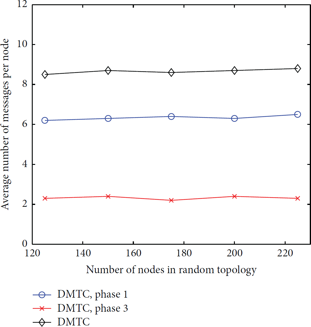
Figure 5 illustrates the number of messages exchanges required per node to complete DMTC in our simulation environment. Recall that the message complexity of the DMTC algorithm is $o\left(N\right)+o\left(S_{N}S\right)$ . For each node, the average number of messages required is $\left(o\left(N\right)+o\left(S_{N}S\right)\right)/N=o\left(\mathrm{1}\right)$ . The result validates the analysis. When the number of nodes in the PSN increases from 125 to 225, the average number of messages required per node in DMTC does not increase. This shows that the DMTC algorithm has little extra overhead.

Figure 5

Number of messages exchanges per node in DMTC when the number of nodes in the PSN increases.

7. Conclusion

We studied the topology control problem in the PSN using an AS approach. The motivation was that the AS network model decouples the complex PSN into simple AS networks. Then we proposed the DMTC algorithm to minimize time delay in the PSN. Compared with most existing approaches where either the purely centralized or the purely distributed control method is adopted, DMTC utilizes a hybrid method. In this way, not only is the control message exchange constrained among local neighboring AS networks, but also the strong connectivity of the network is preserved. Our simulation results validated the theoretic analysis and effectiveness of the DMTC algorithm.

Although the assumptions stated in Sections 2 and 6 are widely used in existing topology algorithms, some of them may not be practical. Our future work will focus on how to relax these constraints (e.g., nodes in the PSN are homogeneous, obstacle-free channel and equal $R_{\mathrm{m}\mathrm{a}\mathrm{x}}$ ) for DMTC algorithm so as to improve its practicality in real applications. In addition, we find that the proposed “hybrid approach” is a general method. It can be extended to solve the control problem of many other large scale networks, for example, machine-to-machine (M2M) network and space information network (SIN). Different topology control algorithms can be applied within AS network and between adjacent AS networks, depending on the optimization objective. And each AS network can be further separated into sub-AS networks. We will study these issues in the near future.