
Abstract
The sensor deployment problem of wireless sensor networks (WSNs) is a key issue in the researches and the applications of WSNs. Fewer works focus on the 3D autonomous deployment. Aimed at the problem of sensor deployment in three-dimensional spaces, the 3D self-deployment (3DSD) algorithm in mobile sensor networks is proposed. A 3D virtual force model is utilized in the 3DSD method. A negotiation tactic is introduced to ensure network connectivity, and a density control strategy is used to balance the node distribution. The proposed algorithm can fulfill the nodes autonomous deployment in 3D space with obstacles. Simulation results indicate that the deployment process of 3DSD is relatively rapid and the nodes are well distributed. Furthermore, the coverage ratio of 3DSD approximates the theoretical maximum value.
1. Introduction
The proliferation of wireless and mobile devices has fostered the applications of wireless sensor networks (WSNs) pervaded from military to industry, agriculture, and other scenarios [1]. The node deployment is a key issue in WSNs, since it seriously influences the feasibility and Quality of Service (QoS) for WSNs. Generally, the node deployment methods can be classified into static deployment scheme and dynamic deployment scheme [2]. And the static deployment schemes are mainly applied in WSNs with nonmobility nodes; it concludes determinate deployment methods and random deployment methods. In the random deployment scenario, sensor nodes are scattered via airplane or other aided measures into the Area of Interest (AOI) to which human being cannot get conveniently. Random static deployment methods ensure the supervision performance via sensor node redundancy. While the dynamic deployment methods are mainly used in a mobile WSNs (i.e., the sensor node has mobility) [3], after being scattered in AOI, the sensor nodes accomplish deployment autonomously. The autonomous deployment of mobile WSNs is a process in which the mobile sensor nodes adjust their positions dynamically according to a certain algorithm, until the predefined coverage requirement is achieved. By adopted dynamic deployment method, the coverage performance is improved, while the overhead of hardware is decreased. However, the self-deployment scheme designing in three-dimension scenario is difficult; aside from this, the obstacle and area boundary may disturb the deployment process. Aimed at solving these problems aforementioned, we proposed a 3D self-deployment (3DSD) algorithm to fulfill the nodes autonomous deployment in 3D area with obstacles. Virtual force model is introduced in 3DSD method. The network connectivity and nodes distribution density are also took into account to provide the feasibility of 3DSD. Extensive simulations are conducted, and experiment results indicate that the deployment duration of 3DSD is comparatively short, and the coverage ratio of 3DSD approximates the theoretical maximum value. The main contributions of our work can be summarized as follows: (1) the virtual force model is extended to three-dimensional space, and the optimal coverage ratio of 3D deployment is defined and calculated, (2) a density control tactic is explored, node density of each cluster is under control to ensure the node distribution of clusters is balance, (3) the network connectivity is concerned, and a negotiation protocol is designed to provide the practicability of 3DSD.
The rest of this paper is organized as follows. A brief introduction to the state of art of the sensor node deployment methods is presented in Section 2. The three-dimensional sensing model and the virtual force model are defined in Section 3. In Section 4, the 3DSD method is described in detail. Performance analysis of the proposed algorithm is provided in Section 5, and conclusions are drawn in Section 6.
2. The State of the Art
For the node deployment in WSN, there are certain coverage performance criteria required to be satisfied. According to the application scenario of WSN, deployment coverage category can be classified into blanket coverage, barrier coverage, and scan coverage [4]. Our work belongs to the blanket coverage.
2.1. Methodology of Deployment
The node deployment is an enabling issue for WSN, so a large number of deployment methods are presented by scholars [5]. There are mainly three categories of research methods in node deployment: incremental deployment method [6], geometric analysis method [7], and virtue force based method [8].
The incremental deployment method is appropriate for the scenario that the prior information of the monitored area is unknown, but the deployment duration is too long. Geometric analysis method cannot guarantee network connectivity, and it is hard to be applied to some scenario with obstacles. Zou and Chakrabarty [8] first proposed deployment method using virtual force model (VFM) in WSN. In VFM, sensor nodes are supposed to be subjected to some kinds of forces which come from area border, other nodes, and so forth. The force balance is regarded as the final state of network. Due to the intuition and the descriptive ability of VFM, it is widely used in deployment issue of WSN [9]. There certainly are some hybrid methods used in node deployment [10].
2.2. Static Deployment and Dynamic Deployment
The node deployment issue can also be classified into static deployment and dynamic deployment according to whether nodes have moving ability. In dynamic blanket deployment, one subissue is how to mend deployment holes formed in static deployment process using mobile nodes [11]. Another subissue is self-deployment of some mobile enabling nodes after they are launched in AOI [12]. Our work focuses on the latter. A geometric analysis method is proposed in [13]; however, there is still the problem that it is hard to be employed in scenarios with obstacles. Zhang and Fei present a deployment scheme to enhance the coverage while keeping the network connected at each step of the deployment [14]. However the obstacle is not taken into consideration. In [15], an autonomous deployment algorithm based on VFM is adopted in 2D scenario. But, for the VFM model with obstacle forces, some certain strategies should be adopted to avoid algorithm trapping into local optimum.
2.3. 3D Surface Deployment and 3D Space Deployment
According to the dimensionality of AOI, the node deployment method can be divided into two classes: deployment in 2D space and deployment in 3D space. In 3D space deployment, there are two subissues, one is 3D area coverage [16] (e.g., underwater sensor deployment) and the other is 3D surface deployment (e.g., mountain surface deployment). An underwater acoustic sensor self-deployment scheme is proposed in [17], which achieved relative good performance. Our work is about the former. A lot of applications of WSN are 3D scenario, so the autonomous deployment of mobile WSN in 3D space is of great significance [18]. It is hard to directly utilize 2D deployment method in 3D space [19]. One kind of solution for 3D coverage or 3D deployment is dimensionality reduction, such that [20] presented an efficient polynomial-time algorithm to solve the coverage problem in three-dimensional wireless sensor networks by translating the problem to 2D and 1D. However, it is not suitable for autonomous self-deployment algorithm. Another solution is to construct the 3D deployment model directly as [21]. However, this centralized method is lack of pervasiveness, because it can only be used in static deployment. Liu et al. [22] proposed a combined virtual force (CVF) algorithm for 3D autonomous deployment, and the performance of this algorithm is good, but the deployment duration is comparatively long.
2.4. The Gap between the Proposed 3DSD and Related Works
The topic of 3D node self-deployment in WSNs has already received considerable attention in the literature. However, our work is different from them because our proposed scheme is comprehensive. There are many practical requirements considered in our work, such as shortening the deployment process, avoiding the local optimum problem [23], handling the obstacles in AOI, and, meanwhile, maintaining the network connectivity.
3. Preliminaries
3.1. Problem Statement
The 3D self-deployment problem can be defined as follows: “Given a connected network of n sensors each of which has a fixed transmission and sensing range respectively, and are placed in a 3D space with a given area boundaries and some obstacles, our goal is to maximize the coverage area using these mobile sensors as rapidly as possible, meanwhile the network connectivity should be provided.” Taking the limited computation capacity into consideration, the deployment scheme should be lightweight. In the node self-deployment process, there may be some local optimum areas due to the obstacles; this situation must also be considered.
3.2. Three-Dimensional Sensing Model
We adopted a sphere perception model that node s is the center, and,

Ideal 3D perception model.
In Figure 1, node P is an arbitrary point in sphere,

Sensor nodes in 3D space.
In the two-dimensional plane, seamless maximum effective coverage area of three circles is acquired when the three circles intersect at one point and their centers constitute a regular triangle. Compared to the two-dimensional plane, the coverage problem in three-dimensional space is more complex, and the best coverage problem in three-dimensional space is proved to be an NP-hard problem [25], but the foundational idea of the best coverage in the three-dimensional space is the same as that in two-dimensional space. First, two definitions are proposed as follows.
Definition 1 (
).
For an arbitrary node

Definition 2 (
).
For an arbitrary node

Next, let us discuss the intersection of four nodes.
Theorem 3.
There are four seamless topological spheres
Proof.
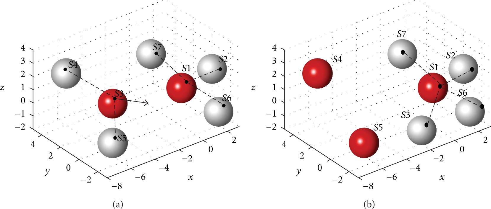
Here we divided the positional relationship of the four sphere centers into two cases. The first one is shown in Figure 3(a); add a ball

The second case is shown in Figure 3(b), and the tetrahedral made up of
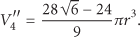
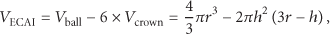
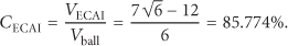
Obviously, it can be seen that the maximum effective coverage space in four balls is obtained when the four sphere centers constitute a regular tetrahedron. According to formulas (2) and (3), the increment of


The center of the sphere location map.
3.3. Three-Dimensional Virtual Force Model
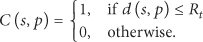
The idea of virtual force model in three-dimensional space is that there are interactive forces between every node in the 3D space. According to the threshold
The formula of the virtual force in three-dimensional space can be described as
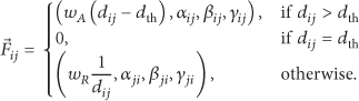
The vector
Force that a sensor node subject to come not only from neighbor sensor nodes but also from obstacles, and this kind of force is treated as repulsion. Due to the repulsion force between node and obstacle, the node is able to be deployed around the obstacle to the open area.

4. Description of 3DSD Algorithm
The design scenario of 3DSD is presented in this section. The explanation and analysis of some design details are also illustrated, such as node density calculating, clustering strategy, and movement location calculation. Finally, we explain the concrete execution steps of 3DSD.
4.1. Assumptions
The 3DSD algorithm is a theoretical model in 3D space. All the sensor nodes have mobility. To highlight the emphasis, some assumptions are proposed as follows.
The sensing area of each sensor node is a sphere; furthermore, the sensing radius and communication radius of each node are equivalent. Each sensor node has mobility and also has the ability to calculate distance and angle using received signal strength and direction. Each sensor node can detect obstacles in its communication scope and can estimate the relative position of obstacles. The travelling speed of each node is very fast, so the time consumption of single movement of node can be ignored. The sensor node movement in its route would not be hindered by other nodes.
4.2. Density Calculation
The magnitude of virtual force is determined by density of nodes and obstacles. The spherical communication area of the sensor node is divided into k subareas evenly, and the value of k is larger, and the expression of density is more accurate. A partition of certain sensor communication area (

Node's communication area partition (
(1) The node density of


(2) The density of an obstacle is defined as

The node density of area 2 (or area 8):
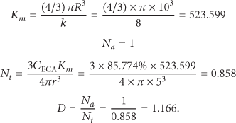
In area 5:

There is one node in area 2 and area 8, respectively, so the node density of these two areas is equivalent. While the number of nodes in the other six areas is 0, the node density is 0. Similarly, obstacle only can be perceived in area 5, so the obstacle density of other areas is 0.
4.3. Clustering Strategy and Density Control
Sensor nodes need clustering to fulfill density control, and the clustering strategy should be simple and efficient to decrease the deployment duration. So, the minimum ID clustering algorithm is adopted here [26].
With nodes movement, there may appear a situation that the member nodes and head node need reselect. As depicted in Figure 5, nodes form two clusters in a certain moment; that is,
Clustering after node moving.
Due to the presence of obstacles, the phenomenon “regional segmentation” may emerge; namely, the force that the nodes are subject to is balanced in local area. To solve this problem, cluster density control is adopted. After clustering is finished, the neighboring head nodes exchange the in-cluster node density. The cluster with higher density schedules some nodes to move in the cluster with lower density, in case the density difference is greater than a certain threshold. To do so, the local force balance is broken, and also the node distribution is more even. The threshold can be determined by the amount of nodes in advance.
4.4. Decision of Target Location
There is a key issue, that is, how to calculate the target location that the node needs to move to. The distance and direction information can be calculated according to the received signal strength and received signal direction, based on the virtual force model proposed in Section 3.2, and we define a virtual force vector


The movement range of a node calculated from resultant force may be very large, and the direction of each node is different. So, after moving, some nodes maybe isolated. Here, a negotiation strategy is adopted to ensure network connectivity.
Node Neighbor node
If there is no effect on network connectivity after movement of If the new position of If the new position of Node
If there is no “alert” message sent back and numbers In case that there is some “alert” message sent back, the minimum suggested distance
To do so, there are at least two one-hop neighbors of
4.5. Description of 3DSD
Each node maintains two types of states; one is cluster state, and the other is node state. The cluster state has three substates: “undecided state,” “cluster head,” and “membership,” while the node state has two substates: “undeployed” and “deployed.” The node state is used to distinguish whether the nodes have been deployed in present round. Arguments of 3DSD are listed in Table 1.
Input arguments of 3DSD.

The pseudocode of 3DSD is provided in Algorithm 1. Here,
Initiated While (there are some nodes moved in the last round) {For each node i sent( update adjacency list calculate D and sent( negotiation process For each node i if ( {move to the destination if (there is obstacle in the planed path) change destination to the surface of the obstacle} re-clustering For each cluster-header Cluster density balancing process }
5. Simulation and Analysis
5.1. Simulation Environments
The size of the AOI is set as 80 m × 80 m × 80 m. In order to calculate the volume of the obstacles and the coverage ratio, the AOI is divided into grids, and the region area is 1 m × 1 m × 1 m. We assume that the sensing range is 10 m, and the communication range is 20 m. In the simulation, the success rate of sending and receiving messages is 100%. There are several obstacles in this three-dimensional space, and they are randomly placed, and in order to facilitate the calculation of obstacle density, the shapes of the obstacles are set as rectangular in simulation. The boundaries of the three-dimensional space are also treated as an obstacle.
5.2. Effect and Evaluation
In the three-dimensional space with obstacles, 120 nodes are scattered randomly in the center of the area. Then, the deployment commences. These 120 nodes finally are deployed evenly to the whole space under the functions of attraction and repulsion, and the effect of the algorithm implementation is shown in Figure 6. The ID distribution of cluster head node during the algorithm execution is shown in Figure 7. In the figure, the abscissa represents the ID number, and the ordinate indicates the times the node was selected as cluster head in the total 30 deployment rounds. Algorithm has performed twice as illustrated in Figures 7(a) and 7(b), we can see the difference of the two results of execution, this is because the nodes are randomly placed in initialization stage, and different initial position will lead to forming different cluster during the algorithm execution. Density control strategy is used in 3DSD. Changes of the average density during the implementation are shown in Figure 8. The abscissa is deployment rounds, and the ordinate is the average density of clusters. From the beginning, there is high density because nodes are concentrated, slow nodes start to spread out, density becomes lower and lower, and node density between clusters tends to be balanced. Two most important indicators to assess deployment algorithm are coverage ratio and deployment rounds. Figures 9 and 10 are the results of the execution of 3DSD. Still in the previous environment of 3D space, the number of nodes increased from 5 to 120, the abscissas are number of nodes, and the ordinate is the coverage ratio and deployment rounds, respectively. We can see that with the gradual increase of the number of nodes, both coverage and deployment rounds show ascendant trend. The number of nodes is in a linear relationship with the coverage, and the number of nodes is proportionate to the deployment rounds. When there are 120 nodes in the AOI, the highest coverage rate can reach 82%. But the theoretical calculated value of the highest coverage rate is 88%; nearly 6% of the error is caused by the system parameter setting and the too big grid.

Execution effect of 3DSD.

ID distributions of cluster head node.

Average node density variation.

Coverage ratio variation.

Deployment round variation.
5.3. Comparison with CVF
The CVF algorithm [22] also focuses on how to maximize the coverage ratio in 3D space by autonomous tactic. Comparisons are conducted between the CVF and our 3DSD algorithm. The two comparison indicators are coverage ratio and deployment time (i.e., deployment duration), as shown in Figures 11 and 12, respectively. The network coverage performances of these two methods are similar. The deployment rounds of these two methods are both increasing with the number of sensor nodes increased. But, the deployment time of 3DSD is less than the CVF. The reasons are that clustering and density control tactics are introduced in 3DSD, and the terminal criteria of 3DSD are threshold judgment, while the terminal criteria of CVF are round-movement judgment. Note that the time of deployment becomes important when the coverage ratio of deployment algorithm is close to the theoretical maximum.

Comparison of coverage ratio.

Comparison of deployment variation.
5.4. The Flexibility of 3DSD
In previous subsection, the rapid deployment feature of 3DSD is indicated. The terminal criteria of deployment are related to value of ω. When the amount of sensor nodes is enough to fully cover the AOI, we can adjust the value of ω to speed up the deploying process as illustrated in Figure 13. The amount of nodes is 200 in the identical area, and the value of ω varies from 10% of sensing radius to 30% of it. As we can see in Figure 13, in all of these five cases with different ω, the coverage is the same, that is, 100%. However, the deployment duration is shortened along with ω increase.

Iterations versus value of ω.
This result shows that 3DSD has flexibility, and it can provide rapid deployment for different initial condition.
6. Conclusion
A distribution autonomous deployment algorithm 3DSD is proposed in this paper. Aimed at the node deployment issue in 3D space, the virtual force model is adopted in 3DSD. The forces coming from boundaries of AOI, obstacles in sensing area, and the sensitive area are totally considered. The negotiation strategy is introduced to provide network connectivity. The node density control scheme is adopted such that the density between clusters is balanced. Simulation results show that the performance of 3DSD is preferable, and the coverage ratio of 3DSD is quite high.
The work focus on 3D autonomous deployment for WSN situates initially theoretical stage yet. In the future, the following issues should be considered: (1) to construct the 3D irregular sensing model, (2) to introduce error eliminating methods for computing and moving, and (3) to evaluate the feasibility of 3D node deployment algorithm in field experiment.
Footnotes
Conflict of Interests
The authors declare that there is no conflict of interests regarding the publication of this paper.
Acknowledgment
This research was supported by The National Natural Science Foundation of China (61379023).