On the Use of Perfect Sequences and Genetic Algorithms for Estimating the Indoor Location of Wireless Sensors

Abstract

Determining the indoor location is usually performed by using several sensors. Some of these sensors are fixed to a known location and either transmit or receive information that allows other sensors to estimate their own locations. The estimation of the location can use information such as the time-of-arrival of the transmitted signals, or the received signal strength, among others. Major problems of indoor location include the interferences caused by the many obstacles in such cases, causing among others the signal multipath problem and the variation of the signal strength due to the many transmission media in the path from the emitter to the receiver. In this paper, the creation and usage of perfect sequences that eliminate the signal multipath problem are presented. It also shows the influence of the positioning of the fixed sensors to the precision of the location estimation. Finally, genetic algorithms were used for searching the optimal location of these fixed sensors, therefore minimizing the location estimation error.

1. Introduction

The GPS (Global Positioning System) receivers work well in line-of-sight (LOS) conditions, meaning they cannot be used in an indoor scenario or locations in which there is limited LOS to the GPS satellites. Current GPS outdoor location accuracy is around 3 meters and is too high for most home automation purpose tasks. Additionally a GPS signal cannot be caught clearly in indoor scenarios.

The type and quality of measurements have a considerable effect on the performance of a positioning algorithm in a Wireless Sensor Network (WSN). Different types of measurements have been considered in the literature [1] for the positioning problem, for example, received signal strength (RSS), angle-of-arrival (AOA), time-of-arrival (TOA), and time-difference-of-arrival (TDOA). The application of such techniques can be found in [2].

Since designing an estimator for the positioning problem strongly depends on the model of measurements, it is of great importance to use an accurate model for measurements. The sensor nodes can be either stationary or moving. They might also be able to make more than one type of measurement. Our project started with RSS-based measurement because it is the only accepted measurement that does not suffer from NLOS conditions. Our real scenario work instance is a building with a considerable set of walls where a wireless sensor should be able to locate itself.

The performance of communication systems using Code Division Multiple Access (CDMA) and Orthogonal Frequency Division Multiple Access (OFDMA) is directly related to the coding sequence they use. These sequences should have a perfect autocorrelation and excellent cross-correlation properties for synchronization or code detection in noisy environments. The importance of code detection accuracy in these coding sequences becomes evident when they are applied in WSN environments that have much interference.

In this paper, the general issue of implementing an accurate Indoor Positioning System (IPS) will be tackled, using a small TDM-CDMA (Time Division Multiplexing-Code Division Multiple Access) distributed sensor network. This IPS system will be implemented using low cost FM (Frequency Modulation) transmitters and receivers.

Several sequences have been proposed and used in communication and localization systems. In the third generation of mobile communication (3G), Walsh-Hadamard sequences are used in UMTS [3]. This system has been further improved in what is now called 4G Long Term Evolution (LTE), using Zadoff-Chu sequences instead of the Walsh-Hadamard [3]. Another set of sequences, the Gold sequences, are currently used in the Global Positioning System (GPS) for outdoor localization [4]. Golay sequences are also widely considered in many areas, including radar systems [5].

An analysis was performed by comparing the behavior of novel OPDG (Orthogonal Perfect DFT Golay) codes to the ZigBee codes (32-length Pseudo Noise code of a WSN), demonstrating that OPDG codes have better correlation properties. Afterwards, a scenario of an IPS is set up, and the significance of using OPDG codes with better correlation properties is presented. We start the paper by explaining the intention of using a novel code family (OPDG), comparing it to the well-known PN (Pseudo Noise) ZigBee codes. Afterwards, a scenario of our IPS system is introduced, and testing results are presented. To further improve the IPS system, we introduce a genetic algorithm that helps us locate the optimum FM transmitter placement positions within the indoor scenario.

At the end, it is pointed out how the presented results indicate that this system is a viable alternative to existing IPS systems, with the additional advantage of its low implementation cost.

2. OPDG IPS Model

One of the major problems of wireless communication is multipath interference (MPI). Transmission media, such as wireless, can bounce off certain obstacles, taking multiple paths to reach the receiver. Delays created by these obstacles can cause interference in communication. Other interferences include the multicarrier interference, intersymbol interference, and the multiple access interference. These interferences can be reduced by using perfect sequences for transmission [6]. The latter two interferences can be reduced if those sequences are also orthogonal for any delay between them [7].

Our task is to improve accuracy in IPS systems that use wireless communication. In indoor wireless communication, the use of code sequences that are resistant to multipath interferences is vital to achieve accuracy, due to a large number of obstacles present in the environment. We propose the use of perfect sequences, whose correlation properties render them immune to multipath interferences, as opposed to commonly used coding sequences.

In this section, autocorrelation and cross-correlation properties of coding sequences will be explained. Further on, a comparison will be made between the widely used ZigBee coding sequences and the novel OPDG sequences. Lastly, a low cost IPS scenario will be set up and explained.

2.1. Autocorrelation and Cross-Correlation

A sequence is a periodic sequence with a period M when $x(n)=x(\mathrm{mod}(n,M))$ , where $\mathrm{mod}(a,b)$ is the remainder of a divided by b.

Let $x[n]$ with $n=\mathrm{0,1},2,\dots ,M-1$ be one of the M values of a periodic sequence x. The DFT (Discrete Fourier Transform) of $x[n]$ is defined as

$$\begin{array}{cc}& X\left[k\right]=\text{DFT}\left\{x\left[n\right]\right\}={{\displaystyle \sum }}_{n=\mathrm{0}}^{M-\mathrm{1}}x\left[n\right]W_M^{kn},\end{array}$$

(1)

where $W_M$ = exp $(-j2\pi /M)$ , $k=\mathrm{0,1},2,\dots ,M-1$ , with $j=\sqrt{-1}$ for convenience of notation. The IDFT (Inverse Discrete Fourier Transform) of $X[k]$ is then given by

$$\begin{array}{cc}& \text{IDFT}\left\{X\left[n\right]\right\}=x\left[n\right]=\frac{\mathrm{1}}{M}{{\displaystyle \sum }}_{k=\mathrm{0}}^{M-\mathrm{1}}X\left[k\right]W_M^{-kn}.\end{array}$$

(2)

Using (1) and (2), the periodic cross-correlation between two different sequences $x^{(r)}$ and $x^{(s)}$ is defined as

$$\begin{array}{l}{R}_{x^{\left(s\right)}{x}^{\left(r\right)}}\left[n\right]={{\displaystyle \sum }}_{k=\mathrm{0}}^{M-\mathrm{1}}{x}^{\left(r\right)}\left[k\right]x^{\mathrm{\ast }\left(s\right)}\left[\mathrm{mod}\left(k+n,M\right)\right]\\ \hspace{1em}\hspace{1em}\hspace{1em}\hspace{1em}={{\displaystyle \sum }}_{k=\mathrm{0}}^{M-\mathrm{1}}{x}_k^{\left(r\right)}{x}_{k+n}^{\mathrm{\ast }\left(s\right)}.\end{array}$$

(3)

Alternatively, it can be defined as

$$\begin{array}{cc}& R_{x^{\left(S\right)}{x}^{\left(r\right)}}\left[n\right]=\text{IDFT}\left\{X^{\left(r\right)}{X}^{\mathrm{\ast }\left(s\right)}\right\},\end{array}$$

(4)

where the superscript $\mathrm{\ast }$ denotes the complex conjugate.

The autocorrelation of a periodic sequence can also be calculated using (4), when $r=s$ .

When a periodic sequence has an autocorrelation of zero for any nonzero delay, the sequence is said to be a perfect sequence. Additionally, the two different sequences are called orthogonal if the cross-correlation between them is zero for a null delay. Because of these correlation properties, orthogonal perfect sequences are ideal to be used in several applications, such as radar systems, sonar systems, and communication synchronization systems.

2.2. OPDG Code

Any sequence set with perfect or near-perfect autocorrelation values, which is also orthogonal or near-orthogonal, is a good candidate to be used in asynchronous communication systems, such as DS-CDMA (Direct-Sequence Code-Division Multiple Access), or any other system where the signal reception may be contaminated by the multipath problem. Another important property for the sequence set is the number of orthogonal sequences available. The Gold sequences are a good example of a set of sequences having these properties, since they have excellent correlation properties while being possible to generate in large numbers. For instance, it is possible to create 32 orthogonal Gold sequences with a length of 32. However, sequences with low cross-correlation values usually have high out-of-phase autocorrelation values. Likewise, low out-of-phase autocorrelation values are usually achieved at the cost of higher cross-correlation values. A compromise between these properties must be carefully selected for usage on a CDMA-based communication system.

Golay sequences are bipolar complementary sequences. Additionally, the autocorrelation of a single sequence of a Golay pair is not zero with all non-null delays, for any length $L=2^N$ . However, the sum of the out-of-phase autocorrelations of both sequences in the pair is zero. Therefore, Golay sequences are not perfect sequences. Nevertheless, they are interesting for their properties. A generic algorithm for Golay sequence generation was presented by Budisin [8] as follows:

$$\begin{array}{cc}& a_{\mathrm{0}}\left[k\right]=\delta \left[k\right],\\ b_{\mathrm{0}}\left[k\right]=\delta \left[k\right],\\ a_n\left[k\right]=a_{n-\mathrm{1}}\left[k\right]+w_n{b}_{n-\mathrm{1}}\left[k-D_n\right],\\ a_n\left[k\right]=a_{n-\mathrm{1}}\left[k\right]-w_n{b}_{n-\mathrm{1}}\left[k-D_n\right],\end{array}$$

(5)

where $\delta [k]$ is the unit pulse function that works as a trigger signal, $a_n[k]$ and $b_n[k]$ are the Golay sequences, $w_n$ is a generation seed (either 1 or −1), and $D_n$ is a delay $(2^{n-1})$ .

An example of a Golay complementary sequence of length 4 is the following pair: $(+1,+1,+1,-1)$ and $(+1,+1,-1,+1)$ . The amplitude of a Golay sequence $a_n[k]$ is a constant value given by $\left|a_n[k]\right|=1$ .

It is well-known that any constant amplitude sequence, defined in the frequency domain, corresponds to a perfect sequence in the time domain.

Applying an IDFT to Golay sequences creates two new polyphase perfect sequences, which are

$$\begin{array}{cc}& \text{OPD}{\text{G}}_{\mathrm{1}}=\text{IDFT}\left\{a_n\left[k\right]\right\},\\ \text{OPD}{\text{G}}_{\mathrm{2}}=\text{IDFT}\left\{b_n\left[k\right]\right\}.\end{array}$$

(6)

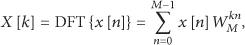
It should be noted that it is possible to find the IDFT of any sequence X using also a DFT, because

$$\begin{array}{cc}& \text{IDFT}\left\{X\left(n\right)\right\}=\frac{\mathrm{1}}{N}{\left[\text{DFT}\left\{X^{\mathrm{\ast }}\left(n\right)\right\}\right]}^{\mathrm{\ast }}.\end{array}$$

(7)

The same sequences can be achieved by a recursive algorithm as follows:

$$\begin{array}{cc}& a_{\mathrm{0}}\left[k\right]=A,\\ b_{\mathrm{0}}\left[k\right]=A,\\ a_n\left[k\right]=a_{n-\mathrm{1}}\left[k\right]+q·W_{{\mathrm{2}}^N}^{-k·{\mathrm{2}}^{n-\mathrm{1}}}·b_{n-\mathrm{1}}\left[k\right],\\ b_n\left[k\right]=a_{n-\mathrm{1}}\left[k\right]-q·W_{{\mathrm{2}}^N}^{-k·{\mathrm{2}}^{n-\mathrm{1}}}·b_{n-\mathrm{1}}\left[k\right],\end{array}$$

(8)

where A is a constant signal or vector, $W_L$ = exp $(-j2\pi /L)$ , $j=\sqrt{-1}$ , and $0<n\le N$ . The resulting sequences $a_n$ and $b_n$ are the OPDG₁ and OPDG₂ as per (6) scaled by $A\times L$ . They can be on the same scale as (6) using $A=1/L$ , with $L=2^N$ .

Several operations can be applied to the OPDG sequences to generate different sequences. One can create a real code by ignoring the imaginary part of the complex valued sequences and keeping only the real part $(\mathrm{Re}\{{\text{OPDG}}_x\})$ . Likewise, one can ignore the real part of the sequence and keep only the imaginary part $(\mathrm{Im}\{{\text{OPDG}}_x\})$ . One can also add the real part to the imaginary part ( $\mathrm{Re}\{{\text{OPDG}}_x\}$ + $\mathrm{Im}\{{\text{OPDG}}_x\}$ ). It is also possible to apply a sign function to any of the previous sequences. A sign function (Sgn(x)) returns −1 to negative inputs and 1 to positive ones. Another possibility is to make a cyclic shift of the imaginary part of each code, prior to the sum, thus generating $L-1$ new complex valued sequences.

It is also possible to decode the original input value A, from (8), back from the OPDG codes. A recursive decoding method can be used as follows:

$$\begin{array}{cc}& a_{n-\mathrm{1}}\left[k\right]=q·W_{{\mathrm{2}}^N}^{-k·{\mathrm{2}}^{n-\mathrm{1}}}·\left\{a_n\left[k\right]+b_n\left[k\right]\right\},\\ b_{n-\mathrm{1}}\left[k\right]=a_n\left[k\right]-b_n\left[k\right],\end{array}$$

(9)

where $1\le n\le N$ , $a_n$ and $b_n$ are the OPDG₁ and OPDG₂ that resulted from (8), and, as previously, $W_L$ = exp $(-j2\pi /L)$ . Notice that, in (9), n varies from N down to 1. From $a_0$ and $b_0$ , a vector $A^{\prime }$ can be created by

$$\begin{array}{cc}& A^{\prime }\left[k\right]=a_{\mathrm{0}}\left[k\right]+b_{\mathrm{0}}\left[k\right].\end{array}$$

(10)

The resulting $A^{\prime }$ is an interesting vector because it presents two different method decoding processes:

$$\begin{array}{cc}& \mathrm{Re}\left\{\text{DFT}\left(A^{\prime }\right)\right\}=A{\left[q\right]}^N{\mathrm{2}}^{\mathrm{2}N+\mathrm{1}}\delta \left[k-{\mathrm{2}}^N+\mathrm{1}\right],\end{array}$$

(11)

$$\begin{array}{cc}& {\left|A^{\prime }\right|}^{\mathrm{2}}=A^{\mathrm{2}}{\mathrm{2}}^{\mathrm{2}N+\mathrm{2}}.\end{array}$$

(12)

As seen in (11), the real part of a DFT applied to $A^{\prime }$ is proportional to a Dirac pulse delayed by $2^N-1$ . This property allows an enhanced detection process in spite of MPI.

2.3. Usage in the ZigBee Communication System

The novel OPDG codes are derived from real orthogonal perfect DFT sequences. To be more precise, the first OPDG code is obtained by making the sum of the real and imaginary part of OPDG₁. The second OPDG code is built using the addition of the real and imaginary part of OPDG₂. These novel codes are real, orthogonal, and perfect. As such, they should be optimum alternative codes for a ZigBee communication system, which uses PN codes defined in [9, 10].

An autocorrelation crest factor can be used as a parameter of autocorrelation efficiency. The autocorrelation crest factor ACCF is defined as a ratio of the maximum peak $A_{\text{peak}}$ and the root mean square of the autocorrelation function $A_{\text{rms}}$ as

$$\begin{array}{cc}& \text{ACCF}=\frac{A_{\text{peak}}}{A_{\text{rms}}}.\end{array}$$

(13)

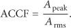
When the autocorrelation is perfect, like a Dirac pulse, the ACCF of a periodic sequence of length L is equal to $\sqrt{L}$ .

A comparison between these two codes is as follows. Figure 1 shows the normalized periodic autocorrelation properties of the standard ZigBee codes with the code length of 32. The ACCF average is 7.77. Figure 2 shows the normalized periodic autocorrelation properties of the OPDG codes with the length of 32. The ACCF average is 9.48. Furthermore, by increasing the code length, autocorrelation properties (or ACCF) increase greatly. Increasing the code length of the OPDG codes results in a reduction of fluctuation in the normalized periodic autocorrelation function, as can be seen in Figure 3. This last ACCF average, 18.62, is much higher.

Figure 1

Normalized absolute periodic autocorrelation, ZigBee PN codes, with resolution of 16 bits.

Figure 2

Normalized absolute periodic autocorrelation, OPDG codes, with resolution of 16 bits.

Figure 3

Normalized absolute periodic autocorrelation, OPDG codes with the code length of 128, with a resolution of 16 bits.

As it may be observed, the novel OPDG codes have better correlation properties despite using a simple 16-bit resolution.

2.4. Indoor Positioning System

Building an IPS system that would enable us to accurately determine the position of an entity in a closed space, with a lot of MPI, is a difficult problem in positioning systems. We believe that the use of the OPDG codes can greatly enhance the accuracy of low cost IPS systems that use CDMA.

We propose a system that can use the communication of FM transmitters and receivers with OPDG codes to determine the indoor location of a device. The computing device we use to receive and process the codes is a small, low-powered single-board computer Raspberry Pi [10]. A second Raspberry Pi is also used to control the transmissions of all emitter pairs.

Our system is depicted by Figure 4, where each pair transmits its code in TDM. Inside the indoor scenario, FM transmitters are placed in optimum positions to cover the room with as much signal as possible. The Raspberry Pi is mounted on an object that allows its location discovery. As the different FM transmitters emit different OPDG codes, Raspberry Pi uses those codes to approximate the distance to each individual transmitter using the following formula:

$$\begin{array}{cc}& {\widehat{d}}_{ij}=d_{\mathrm{0}}\mathrm{1}{\mathrm{0}}^{(P_{\mathrm{0}i}-\mathrm{10}\log (\text{ACCF}\times A_{\text{rms}}\left)\right)/\mathrm{10}\beta }.\end{array}$$

(14)

Figure 4

IPS network topology.

Equation (14) was derived from the distance estimation equation introduced in [2] and represents the distance between nodes i and j. $P_{0i}$ denotes the power in dB at the distance $d_0$ , β is a path-loss exponent that is usually between 2 and 6 [11], ACCF is the autocorrelation crest factor, and $A_{\text{rms}}$ is the root mean square of the autocorrelation function.

2.5. Use Case Scenario

We have implemented an IPS scenario using a pair of FM transmitters. Each emitter was broadcasting one different real OPDG code of the set {Re[OPDG₁] + Im[OPDG₁] ∪ Re[OPDG₂] + Im[OPDG₂]}. Both FM emitters transmitted 128-length OPDG codes with a total-length of 128 × 4 chips, at 106.9 MHz (mono), with a sample rate of 8000 samples/sec and a hardware resolution of 16 bits. The broadcast was continuous during 30 seconds. FM transmitters were located 7 m away from each other.

Figure 5 shows two theoretical ratios of ACCF values of a pair of OPDG codes. Using this ratio, we can approximate a linear function for the displacement estimation and reduce the error of the IPS. The theoretical worst case ratio of Figure 5 was calculated using all phases of the two FM signals.

Figure 5

Theoretical ACCF1/ACCF2 ratios.

On the other hand, the theoretical best case ratio was achieved considering 2 constructive multipath interferences. These interferences were created by placing a RF (Radio Frequency) reflector 35 cm behind each emitter. Using this scenario, a stationary wave average has less fluctuation and represents the best theoretical case.

This theoretical model shows the possibility of finding a linear function based on the interval around −1.75 m and 3 m.

3. Results and Discussion

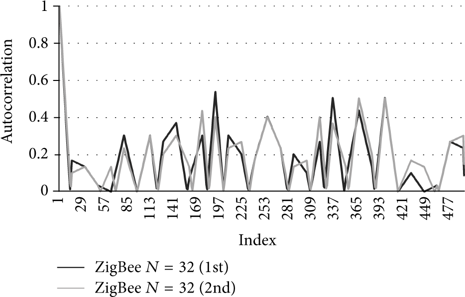
We have implemented the first stage of our low cost IPS testbed and in this section we will present some results. Normalized autocorrelation functions and ACCF parameters are presented in Figures 6 and 7.

Figure 6

Normalized autocorrelationof ZigBee codes, 32-length.

Figure 7

Normalized autocorrelation of OPDG codes, 32-length.

Figures 6 and 7 show the correlation between the received and reference codes within the Raspberry FM receiver. When compared to the ZigBee codes, OPDG codes with the length of 32 can reveal an ACCF 40% higher and therefore substantially better. Figure 8 shows the correlation of 128-length OPDG codes. Peaks are distinguishable and the fluctuation is significantly lower. Its better autocorrelation properties enable better approximation of the crest factor using (13).

Figure 8

Normalized periodic autocorrelation of OPDG codes, 128-length.

Our IPS measurements of the ACCF are shown in Figure 9. OPDG codes with the same code length as ZigBee codes give an average of 8% better ACCF, while increasing the code length of the OPDG codes to 128 highly improves the ACCF to an average of 7.1. These measurements were made during 30 seconds.

Figure 9

ACCF measurements of different codes.

In the last scenario, a pair of real OPDG codes {Re[OPDG₁] + Im[OPDG₁]} and {Re[OPDG₂] + Im[OPDG₂]} has been used. The first FM emitter of the pair, with the code {Re[OPDG₁] + Im[OPDG₁]}, was located at −3.5 meters of the central point zero. The second FM emitter of the pair, with the code {Re[OPDG₂] + Im[OPDG₂]}, was located at +3.5 meters. Both emitters were in LOS, with some walls around them, creating a real indoor environment with some MPI.

We have tested the theoretical model of the ACCF ratios in a real scenario and have come to the following results. By emitting 2 pairs of 128-length OPDG codes, a decreasing line trend from one FM emitter to the other is visible, as can be seen in Figure 10. Two linear equations are also shown in the figure, along with reliability R.

Figure 10

ACCF ratios of 2 pairs of OPDG codes with FM modulation at a distance of 7 m.

Reliability can be further increased by calculating the average of the functions in Figure 10, as seen in Figure 11.

Figure 11

The average of 2 ACCF ratios of 2 pairs of 128-length OPDG codes with FM modulation at a distance of 7 m.

With two pairs of FM OPDG emitters, we obtain an average IPS error of 0.86 meters, with a maximum error of 2 meters. However, it is possible to predict a lower error if more pairs of emitters can be used around the FM receiver. The correct emitter locations are an open issue that should be solved shortly.

4. Positioning the Sensors Using Genetic Algorithms

The indoor location, as seen in the previous section, is estimated using the received signal strength (RSS) of multiple emitters. The placement of these emitters can have a large influence on the location estimation error of the receiver sensor. In this section, we will show a metaheuristic approach to this signal emitter placement problem, namely, using genetic algorithms.

4.1. Positioning of the Sensors

The emitter placement presents two different problems to solve: how many emitters are needed to cover an area (such as a building or a room) and where to place them so that their signal is best used. The first problem is a standard coverage problem and can be stated as follows: given a site plant, including all possible emitter locations, how many emitters are needed so that every position in that location receives n different signals? This is a minimization problem where the variable to minimize is the number of required emitters.

The second problem is more complex. When a receiver detects n signals it will start the triangulation calculations to estimate its location. However, the resulting precision of that estimation will vary greatly with the source of those signals. Figures 12 and 13 exemplify this problem. These figures represent a simple 4 m × 4 m square room with 3 emitters (represented by triangles in the figures) and 1 receiver (represented by an x). The plus sign (symbol +) represents the location estimation of the receiver considering the RSS of the emitters. The 3 emitted signals cover all the room, so the signal coverage is the same for both figures. In Figure 1, the emitters are close to each other, which makes having 3 signals almost as good as having only 1, resulting in a large location estimation error (above 1 meter). Dispersing the location of the emitters, as shown in Figure 13, results in better conditions to estimate the receiver location. In this example, the theoretical location estimation error is reduced from around 1 meter in Figure 12 to a mere 4 cm in Figure 13. Taking this into account, the second problem consists in finding the best location of n signal emitters so that the location estimation error of a receiver is minimized for all possible receiver locations.

Figure 12

Low precision of the location estimation when the signal sources are too near to each other. The estimation is approximately 1 m away from the true location of the receiver.

Figure 13

High precision of the location estimation when the emitters are scattered around the target location. In here, the estimated location is only 4 cm away from the true receiver location.

Both of the previously described problems can be seen as combinatorial optimization problems. The number of possible combinations is, however, extremely large and would take too long for a computer to calculate and evaluate all of the possible combinations. Since the finding of the optimal solution is very hard, in these classes of problems, one generally accepts a near optimal solution. Metaheuristic algorithms deliver this near optimal solution and have been successfully applied to combinatorial optimization problems. One such algorithm is the genetic algorithm.

4.2. Genetic Algorithms

A genetic algorithm (GA) is a population based metaheuristic search algorithm [12, 13]. Its basic operation is depicted in Algorithm 1. A GA starts by creating an initial population $P_0$ and evaluating it. Then, a new population $P_0^{\prime }$ is created by selecting parents from the original population $P_0$ and applying several different operators to them. These operators are usually crossover and mutation operators. The execution of the GA proceeds to the evaluation of $P_0^{\prime }$ and then combines $P_0$ with $P_0^{\prime }$ , replacing the previous generation of the population ( $P_0$ ) with a new population generation $(P_1)$ . Since the population size is usually immutable during the algorithm execution, this combination is basically a selection of a few members from the old population $P_0$ with the remaining slots being filled with elements of the new population $P_0^{\prime }$ . Selection, modification, evaluation, and replacement operations repeat for many generations until a stopping condition is reached.

Algorithm 1: Pseudocode of a genetic algorithm.

$$n=0$$

$$P_0$$ = generateInitialPopulation()

evaluate( $$P_0$$ )

while not stoppingCondition() do

   $$P_n^{\prime }$$ = selectParents( $$P_n$$ )

   $$P_n^{\prime }$$ = applyVariationOperators( $$P_n^{\prime }$$ )

  evaluate( $$P_n^{\prime }$$ )

   $$P_{n+1}$$ = selectNewPopulation( $$P_n$$ , $$P_n^{\prime }$$ )

  n = n + 1

end while

return the best found solution

With GA being a metaheuristic algorithm, all these operations must be tuned to the problem it will solve. The adaptations that need to be made consist in the definition of the solution representation for the GA, the evaluation and scoring of a solution (also called the fitness calculation), the initial population creation method, the mutation and crossover operators, the parent selection, and the population replacement method.

4.3. Solution Representation

In both emitter placement problems, a solution consists simply in the location of a set of signal emitters. These locations are chosen from a larger set of all possible locations. Visually, this set can be represented as in Figure 14, which shows a small part of a site plant. In this figure, 12 possible locations for signal emitters are presented, with a signal emitter being placed in the 6th location (from left to right). A solution like the one presented can be encoded in a binary string of length n, where n is the number of possible emitter locations. In this bit string, 0 indicates an unused possible location while 1 indicates a used location. The solution in Figure 14 would then be encoded as “000001000000.”

Figure 14

Possible signal emitter locations near a wall. Light gray triangles are the possible locations for the placement of signal emitters, while the dark triangle is a placed signal emitter.

Encoding a solution as a string of bits presents a few advantages: they are easy to encode and decode, they do not require large amounts of memory, and they have a fixed size, independently of the number of signal emitters placed. This encoding also facilitates the mutation and crossover operations. Also, this encoding makes it easy to calculate the number of possible emitter placement combinations: $2^n$ different combinations. This exponential growth of the number of combinations is what makes it impossible to find the optimal solution using classic search techniques, such as brute-force searching.

4.4. Solution Fitness Calculation for the Coverage Problem

The evaluation of a solution regarding the coverage problem is based on a few input parameters: the area and shape to cover, the minimum signal strength detected by a receiver, the power of the signal emitter, and the properties of the transmission media. We define the area and shape as a set of rectangular areas. While this does not allow all possible shapes (circular shapes are impossible with this setup), it does allow a good approximation of them while simplifying the calculations.

For the calculation of the area covered by a single signal emitter, we model the power decay, in dB, of the transmitter with

$$\begin{array}{cc}& P_{ij}=P_{\mathrm{0}i}-\mathrm{10}\beta \log \left(\frac{d\left(x_{i,},x_j\right)}{d_{\mathrm{0}}}\right)+{\eta }_{ij},\end{array}$$

(15)

where $P_{0i}$ is the power at distance $d_0$ , $d(x_i,x_j)$ is the Euclidean distance between $x_i$ and $x_j$ , b is a path-loss exponent, $x_i$ and $x_j$ are the location of the emitter and the signal power measurement location, respectively, and ${\eta }_{ij}$ is a zero mean Gaussian random variable with variance ${\sigma }_{ij}^2$ . ${\eta }_{ij}$ assumes the constant value of zero in our calculation of the signal emitter's coverage. We also reduce the signal power whenever it crosses a wall by 2 dB per 15 cm of wall. We considered all walls to be brick walls and this value was found experimentally.

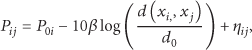
Figure 16 shows a graphical representation of the coverage of 2 signal emitters. In this figure, it is easy to see the effects of walls in the signal power, as well as the overlap of two different signals. After determining the area covered by each and every signal emitter, we calculate the average number of signals in every location in the area (each location is represented by a dot in Figures 15 and 16), as well as the minimum coverage and the standard deviation. The fitness value can then be calculated by

$$\begin{array}{cc}& f=\text{map}\left(\text{avg},\text{curve}\right)+\text{stddev}+\max \left(\text{ideal}-\min ,\mathrm{0}\right),\end{array}$$

(16)

where avg is the average number of signals at every location, curve is the fitness curve shown in Figure 17, $\text{map}(a,b)$ is a function that maps the value a to the corresponding value in the curve b, stddev is the standard deviation of the coverage, $\max (a,b)$ is the mathematical maximum between a and b, ideal is the ideal coverage, and min is the minimum coverage found at all possible locations. The fitness curve shown in Figure 17 allows the guidance of the genetic algorithm by having a clear preference for more signals than ideal over less signals than ideal. Also, the stddev and the $\max (\text{ideal}-\min )$ are penalties applied to the fitness. The first one will guide the GA to solutions where there is no deviation (all locations have exactly the same number of signals covering the location), while the second one heavily penalizes the solution if there are still locations where the ideal number of signals is not reached.

Figure 15

An irregular shaped area approximated by 3 rectangular areas.

Figure 16

Graphical representation of the coverage of 2 signal emitters. Small dots indicate that no signal reaches it; larger dots indicate that the area is covered by at least one signal (larger dots mean more signal coverage).

Figure 17

Fitness curve for the average of the coverage. The horizontal axis is the average number of signals in each location, while the vertical axis is the fitness value.

4.5. Solution Fitness Calculation for the Error Minimization Problem

When considering the minimization of the location estimation error, a different evaluation of possible solutions must be used. Firstly, let us define how the location is estimated. Given a received signal strength s sent from a specific emitter i, according to (15), the distance d of the receiver from the emitter is

$$\begin{array}{cc}& d=d_{\mathrm{0}}\mathrm{1}{\mathrm{0}}^{(P_{\mathrm{0}i}-s+\eta )/\mathrm{10}\beta },\end{array}$$

(17)

where $P_{0i}$ is the power measured at $d_0$ from emitter i, η is a zero mean Gaussian random variable with variance ${\sigma }_{ij}^2$ , and d is the distance of the receiver to the emitter i, given a signal strength of s. Since this distance d depends on the unknown value of η and the signal strength read by the receiver may contain oscillations, one can assume that the receiver is located somewhere in an area defined by an inner circle of radius $d-\epsilon$ and an outer circle of radius $d+\epsilon$ , both centered around the emitter, with ε being a configurable reading precision error. If another signal is read by the receiver, then the receiver location can be restricted to the intersection of the calculated circular areas of both emitters. As the number of signals increases, the intersected area decreases. After all the intersections are made, the estimated location is calculated to be the geometrical center of the resulting area. Figure 18 illustrates this process by showing the inner and outer circles of two received signals, as well as their intersection and estimation of the receiver's location. After estimating the location, its error can be easily calculated as the Euclidean distance between the receiver's real location and the receiver's estimated location. For calculus simplification, we discretize the space into square cells and consider only the center of each cell. This discretization can also be seen in Figure 18, with each dot corresponding to the center of each cell.

Figure 18

Estimation of the location (+) of a receiver (x) using the signal strength of 2 different emitters.

With the estimated location error calculated for each cell, the solution fitness is simply the average of all the errors. Since the error is a Euclidean distance, there will be no negative errors, so an ideal solution would have a fitness of 0, meaning no error at all in any location.

4.6. Mutation Operators

As described in Algorithm 1, the new generation of a population is obtained by applying different operators to selected parents of the current generation. One of those operators is the mutation operator.

During the mutation, each gene can, according to a given probability, maintain its value, flip it, or swap it with another gene. Figure 19 shows an example of a gene's value flip, with the third gene flipping its value from 1 to 0. A gene flip will either increase or decrease the solution's number of emitters. Figure 20 shows an example of a gene swap, where the first gene is swapped with the third gene. A gene swap always maintains the number of emitters but changes their location. The gene swaps always occur between a gene with value 1 and a gene with value 0. This condition guarantees that no unnecessary work is done by the genetic algorithm in the reevaluation of an identical solution.

Figure 19

Example of a gene value flip. On top is the original solution; on bottom is the mutated solution.

Figure 20

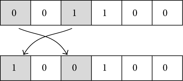
Example of a gene swap. On top is the original solution; on bottom is the mutated solution.

In the coverage problem, the number of emitters varies and must be able to grow or shrink as necessary; thus we use the bit flip mutation. In the error minimization problem, however, the number of emitters is fixed, so the gene swap mutation is applied.

4.7. Crossover Operators

A crossover operator is responsible for recombining the chromosomes of parent solutions into offspring solutions. This process will hopefully combine the best parts of the parents into fitter offspring for the problem.

As with the mutation operators, we must consider crossover operators that may change the number of emitters for the coverage problem and operators that do not change the number of emitters for the error minimization problem. We use a one-point crossover operator in the coverage problem. This operator will randomly select one point on two different parent solutions, split them at that point, and then recombine them into two other offspring solutions. Since the point of crossover is selected blindly, the crossover may increase or decrease the number of emitters in the solution. Figure 21 exemplifies a one-point recombination where the top offspring has less emitters and the bottom offspring has more emitters than the parent solutions.

Figure 21

One-point crossover. On the left are the parent solutions while on the right are the offspring generated by crossing over the parents.

For the error minimization problem, the number of emitters is constant, so a different approach has to be used for the crossover. For this problem, the crossover creates offspring solutions where each emitter is placed from a location of one of the parents. This maintains the number of emitters, while still hopefully using the best parts of each parent solution. Figure 22 shows an example of the application of this crossover to solutions with 2 emitters.

Figure 22

Error minimization problem crossover. This crossover maintains the number of ones in the offspring by selecting ones from any of the parents.

In both problems we select the parents to crossover using a binary tournament selection. In a binary tournament selection two solutions are randomly selected from the population and the best of them (according to their fitness value) is chosen as a parent for the crossover. Doing the selection twice, we get both parents needed for a crossover.

5. Experiments and Results

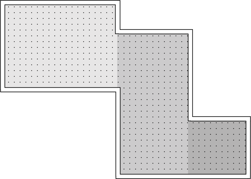
To evaluate the proposed genetic algorithms, we created two different test scenarios. The first test scenario is a long L-shaped corridor of 15 m by 10 m, 3 m wide. In this scenario, the emitters can be placed near the walls with a 25 cm minimum distance between them. Figure 23 shows a map of this corridor along with all the possible emitter locations. The second test scenario is based on the plant of the Telecommunications Institute office at the Polytechnic Institute of Leiria and, as such, represents a real building. In this last scenario we allow the emitters to be near the walls with a 25 cm minimum distance between them as in the last scenario, but we also allow them to be in the ceiling through the middle of each room. Figure 24 shows the map used in this scenario.

Figure 23

Test scenario 1: an L-shaped corridor.

Figure 24

Test scenario 2: the TI office at Polytechnic Institute of Leiria.

We used the genetic algorithms we described for both placement problems and for the two test scenarios. The parameters we used for the genetic algorithm in each problem are detailed in Table 1. The values of these parameters were chosen using some well-known values and fine-tuned while experimenting [14]. The large population size was chosen to have some diversity in the population and it proved to be enough according to our results. We found the stopping criteria of 20000 evaluations to be sufficient to converge the results, as shown by Figure 27. The selection operator (binary tournament) puts pressure on the convergence, while not falling into premature convergence in our experiments, thus being employed. Mutation and crossover operators used were the ones explained in previous sections and were specifically tailored to this problem. The mutation probability was chosen so that, on average, only one bit is mutated per individual, thus not making large changes to each individual. Further studies are required to determine if and how these parameters can be improved. We believe that the convergence speed may be improved, although the rest of the results are technology-dependent. Also, we have discretized the space for the measurements into 50 cm by 50 cm cells. Each measurement was simulated in the center of each cell. Because of the stochastic nature of the genetic algorithm, we ran each experiment 50 times to get statistically valid results.

Table 1

Parameters used in the genetic algorithms.

Parameter	Coverage	Error minimization
Population size	100	100
Stopping criteria	20000 evaluations	20000 evaluations
Selection operator	Binary tournament	Binary tournament
Mutation operator	Bit flip	Bit swap
Mutation probability	1/number of possible emitter locations	1/number of emitters
Crossover operator	One-point crossover	Random emitters from parents
Crossover probability	0.5	0.5

Regarding the coverage problem, the experiment consisted in trying to find the minimum number of emitters to get coverage of 16 signals in each cell. In the first scenario, the GA converged to an ideal solution in every execution after around 12000 solution evaluations. Figure 25 shows the best, worst, and average solution fitness of the 50 runs.

Figure 25

Convergence of the coverage problem genetic algorithm in the first test scenario.

In the minimization of the location estimation error, we instructed the algorithm to place 16 emitters. Figure 26 shows how the average estimation error improved as more solutions were tried by the genetic algorithm. The figure shows that, on average, the location estimation improves in an order of 20%. For the location estimation we set a power reading error of ±5 dB and even with this large error, the algorithm placed the emitters to reduce the estimation error to an average of 15 cm and a maximum estimation error of 43 cm.

Figure 26

Evolution of the solutions in the minimization of the estimation error.

Figure 27

Convergence of the coverage problem genetic algorithm in the second test scenario.

In the second scenario, the results are about the same. Figure 27 shows that, again, the GA finds optimum solutions in the coverage problem, although it took more evaluations (and thus more generations) to reach those solutions.

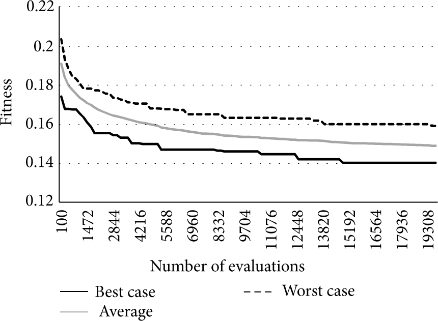
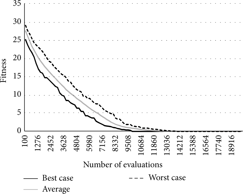
Even though the optimum solution for the minimization of the estimation error with 16 emitters is unknown to us, the GA still shows that it will find good solutions. Figure 28 shows the improvement of the solutions as generations pass.

Figure 28

Fitness of the solutions found during the minimization of the estimation error for the second test scenario.

Although the genetic algorithms appear to give good results, they can be further improved. One such improvement is to join both of the search objectives into a single algorithm, creating a multiobjective algorithm. Such an algorithm will show how the number of emitters affects the precision of the location estimation and also if and when the law of diminishing returns affects that precision.

6. Conclusions

By creating a testbed for a new low cost Indoor Positioning System based on distributed sensor networks, we have to come to encouraging results.

We have shown that the OPDG codes, used in a TDM-CDMA network with a FM modulation, provide better results in an IPS scenario than the ZigBee system, due to its natural immunity to multipath interference.

The new approach with the autocorrelation crest factor shows a way to find a linear function of the distance between the FM receiver and a pair of transmitters, which lowers the error of the IPS. Likewise, the introduction of the genetic algorithm to find the optimum FM transmitter positioning helps in lowering the error and the cost of the IPS.

Results shown in this paper suggest that our IPS system can be further developed to prove itself a viable alternative to existing solutions based on other distributed sensor network technologies.