Analysing Topology Control Protocols in Wireless Sensor Network Using Network Evolution Model

Abstract

In the study of wireless ad hoc and sensor networks, clustering is an important research problem as it aims at maximizing network lifetime and minimizing latency. A large number of algorithms have been devised to compute “good” clusters in a WSN but few papers have tried to characterize these algorithms in an analytical manner. In this paper, we use a local world model to understand and characterize the functioning of three tree based clustering algorithms. In particular, we have chosen simple tree, CDS Rule K, and A3 topology construction protocols. Using our theoretical framework based on a complex network model, we have also tried to quantify some of the observed features of these algorithms such as number of cluster heads and average degree of the resultant graph. The theoretically obtained measures have reasonably matched with measures obtained by simulation studies.

1. Introduction

Wireless sensor networks (WSNs) are made up of a large number of sensor nodes. These nodes are usually deployed in the environment to monitor several physical phenomena. However, sensor nodes heavily depend on batteries as they are the only source of energy in many WSN applications. As a result, one major problem in WSNs is known as topology management that leads to energy efficient transmission of data. In this regard, connections are set with nodes that are close enough for radio signal to arrive with acceptable signal strength. However, in order to improve energy efficiency, topology control process helps in reducing the connections with other neighbors of the node in the network. Topology control is an insistent process in which there is an initialization phase which is common to all WSN deployments. In the initialization phase, nodes make use of the revelation process by using maximum transmission power to build the initial topology. The initial network topology includes connections and nodes that allow direct communication and every node communicates with a subset of the nodes according to the distance between them.

Often, the topology of a large wireless network is structured in terms of a hierarchy where the network is viewed as a number of clusters and in each cluster there is a cluster head and other normal members. Normal members in a cluster communicate only with the cluster heads and the cluster heads communicate with the sink in one or multihop manner. There are many challenges in finding out the “best” set of cluster heads in a given network and, in many formulations, these problems turn out to be intractable. Consequently, there are many algorithms to select the cluster heads and the clusters in a WSN that minimizes latency and maximizes network lifetime.

In many cluster head selection algorithms, every node is selected as the cluster head in different rounds and the probability of selecting a node as a cluster-head is the same for all nodes. In this method, the chances of energy dissipation in cluster heads reduce if we consider large homogeneous WSNs. There are other approaches where the idea of dominating set of graphs is used to devise an algorithm. Some of these approaches are tree based. Most of these algorithms are distributed and work with local (at the most 2-hop) information available from any given node. In this paper, we have considered three such topology construction protocols, namely, simple tree, CDS-Rule K, and A3 protocols for further exploration.

In another development, the theory complex networks have recently received increasing attention for understanding the topological structure, functions, and dynamical properties of many real-world networks such as the social networks, biological networks, and ad hoc networks. One of the most important models that can be used to formally characterize clustering algorithms is known as B-A model [1]. This model is based on two foundational mechanisms: growth and preferential attachment. A new node is added to the network at each step and connects with an existing node with a specific probability, which is related to the degree of the existing node. The B-A network has the scale-free property and follows the power-law distribution.

The B-A network model is capable of capturing some basic mechanism that is responsible for the power-law degree distribution. Still, it had many limitations. Li-Chen model [2] has improved upon B-A model. This model has been able to better capture the dynamics of networks constructed with a local preferential attachment mechanism.

The local preferential attachment model [3] is based on the common sense that people can collect information easily from their local community than from far away environment. Using preferential connection as the fundamental basis, many variations of the scale-free network model have been proposed during recent years such as comprehensive multilocal-world model [4]. Similar to preferential attachment model, the physical position neighbourhoods' model [5] mimics the actual communication network. The Poisson growth model [6] uses the number of edges added at each step as a random variable that corresponds to Poisson distribution. This model can generate many kinds of networks by controlling the random number.

Chen et al. [7] have studied an evolving mechanism for formalizing fault-tolerant communication topology among cluster heads with complex network theory. Based on the B-A model's growth and preferential attachment mechanisms, they not only used a local-world strategy for the network when a new node was added to its local-world but also selected a fixed number of cluster heads in the local world, for the purpose of obtaining a good performance in terms of random error tolerance.

Luo et al. [8] performed theoretical analysis and conducted numerical simulation to explore topology characteristics and network performances with different energy distributions among nodes. Their results have shown that the network is better clustered and average path length for transmitting data is reduced when energy distribution among nodes is more heterogeneous.

In [8], a new dimension is added as the nodes are not only allowed to join the network through preferential attachment but they are also allowed to leave the network or not join the network through nonpreferential attachment. Further the nodes distinguish themselves as cluster head nodes and normal nodes which is consistent with the function of many clustering algorithms in WSNs.

In this paper, we have tried to provide a formalism for some algorithms which computes clusters in a WSN using a modified local network model based on similar models proposed in [2, 9] and [8]. In particular, we have used three tree based clustering algorithms, namely, simple tree, CDS Rule K, and A3. Using our theoretical framework, we have also tried to quantify some of the observed features of these algorithms such as number of cluster heads and average degree of the resultant graph. The theoretically obtained measures have reasonably matched with measures obtained by simulation studies.

The paper is organized as follows. Section 2 describes a very brief review of the local-world model. In Section 3, we have described the application of local world model to provide a framework to describe the functioning of three clustering algorithms. In Section 4, results of theoretical results and simulation studies are jointly presented. Section 5 concludes the paper.

2. A Brief Review of Topology Control Protocols and Local-World Network Model

In this section, we shall discuss very briefly the Li-Chen model [2] and two topology control protocols which are used in this paper.

2.1. A3 Protocol [10]

The A3 protocol uses four types of messages: Hello message, children recognition message, parent recognition message, and sleeping message. The sink node starts the protocol by transmitting an initial hello message to its neighboring nodes. Nodes accept the message if they have not been covered by another node; they set their states as covered, select the transmitter as its parent node, and answer back with a parent recognition message. If a parent node does not get any parent recognition messages from its neighbors, it turns off. The parent node sets a timeout period to accept answers from its neighboring nodes. Once timeout occurs, the parent node sorts the list of neighbor accepting its message in decreasing order of some selection metric. Then, parent node broadcasts a children recognition message that includes the complete sorted list to all its candidates. Once the children accept the list, they set a timeout period proportional to their position on the candidate list. During that timeout they wait for sleeping message from their brothers. If a node accepts a sleeping message during the time out period, it turns itself off.

2.2. CDS Rule k Protocol [11]

The CDS Rule k algorithm utilizes connected dominating set algorithm and pruning rules. The idea is to start from a big set of dominating nodes that produces a minimum criterion and prunes it according to a particular rule. In the first stage, the nodes will interchange their neighbor databases. A node will remain progressive if there is at least one pair of separated neighbors. In the second stage, a node chooses to unmark itself if it determines that all its neighbors are covered by marked nodes with higher precedence, which is given by the degree of the node in the tree. Lower level implies higher precedence. The ultimate tree is a more compact version of initial one with all redundant nodes with higher or equal priority removed.

2.3. Local Network Model

We have used Li-Chen Model [2]. This model is used to form a generalized local-world model. Using the generalized model, we have analyzed clustering algorithms of wireless sensor networks. In this model, each node has only local connection information. Nodes connect only in their local world based on their local connectivity. The following parameters are required to explain the dynamics with reference from Figure 1.

• (1)

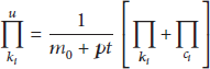
We start from a small number of nodes $m_0$ and grow at each time step t.

(2)

When a new node chooses a connection to other nodes, the probability, $\prod k_i$ , that a new node is connected to a node i depends on the degree $k_i$ of node i. This probability is defined as follows:

$$\begin{array}{cc}& {\displaystyle \prod }\left(k_i\right)=\frac{k_i}{{\sum }_j{k}_j}.\end{array}$$

(1)

(3)

We select M nodes randomly from the existing network which is referred to as local world of the new node.

(4)

When a new node arrives, we add that node with m edges, linking the new node to m nodes in the local world determined in (3) using preferential attachment with a probability ${\prod }_{\mathrm{l}\mathrm{o}\mathrm{c}\mathrm{a}\mathrm{l}}(k_i)$ . This probability is defined as follows at every time step t. Consider

$$\begin{array}{cc}& {\displaystyle \prod }_{\text{local}}{k}_i={{\displaystyle \prod }}^{\prime }\frac{k_i}{{\sum }_j{k}_j},\end{array}$$

(2)

 

where ${\prod }^{\prime }(i\in \mathrm{L}\mathrm{o}\mathrm{c}\mathrm{a}\mathrm{l}-\mathrm{W}\mathrm{o}\mathrm{r}\mathrm{l}\mathrm{d})=M/\left(m_0+t\right)$ .

Figure 1

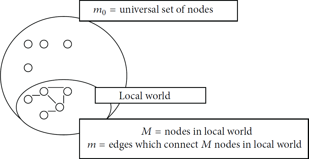
Illustration of various parameters in their roles as describing the local world and the universe.

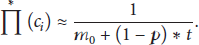
After t time steps, there will be a network with $M=t+m_0$ nodes and $m\ast t$ edges.

3. Applying Local-World Model in WSN Topology Control Algorithms

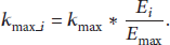
To use local world model to capture functioning of WSN clustering algorithm, the model has to take into account two types of nodes: normal nodes and cluster nodes. The cluster nodes are the cluster heads and the normal nodes are members in a cluster. There is only one cluster node attached to a normal node; in other words, the normal node has only one edge, which means that the normal node cannot relay data from other nodes. A cluster node can integrate and transmit data from other nodes. Both of these two types of nodes can connect to a cluster node and the number of edges is limited in every cluster node because of its energy consideration. When a new cluster node joins the network, it is randomly assigned an initial energy $E_i$ from the interval $[E_{\mathrm{m}\mathrm{i}\mathrm{n}},E_{\mathrm{m}\mathrm{a}\mathrm{x}}]$ . The limited number of edges in every cluster node is represented by $k_{\text{max\_}i}$ , which is based on the initial energy of the cluster nodes $E_i$ where $k_{\mathrm{m}\mathrm{a}\mathrm{x}}$ [12] is given as follows:

$$\begin{array}{cc}& k_{\text{max\_}i}=k_{\mathrm{m}\mathrm{a}\mathrm{x}}\ast \frac{E_i}{E_{\mathrm{m}\mathrm{a}\mathrm{x}}}.\end{array}$$

(3)

$k_{\text{max\_}i}$ reflects the ability of having the maximum number of edges for cluster node i.

The growth model is described as follows. Starting with a small number of nodes (all of them are cluster nodes), they randomly link each other. This results into an initial network.

• (1)

Growth. At every time step, a new cluster node or a normal node with one edge enters into the existing network with a probability p or $1-p$ , respectively. If the new node is a cluster node then it is assigned a random energy value of $E_i$ as discussed. A small number of cluster nodes would cause many sensor nodes to link to them, which results in faster energy consumption; but a large number of cluster nodes would be more wasteful in terms of energy efficiency. Thus, the value of p is assumed to be in the range as $0<p<0.5$ .

(2)

Preferential Attachment. A new node arriving at the network links to an old cluster node that is selected randomly from the already existing network. Nodes in WSNs have the constraint of energy and connectivity and only communicate data with the cluster nodes in their local area. First, M cluster nodes are selected randomly from the network as the new incoming node's local world; then, one of the cluster nodes is chosen to link with the new node according to the probability ${\prod }_{\mathrm{l}\mathrm{o}\mathrm{c}\mathrm{a}\mathrm{l}}^{}(k_i)$ .

If the new incoming node is a cluster node, then the probability is set as follows:

$$\begin{array}{cc}& {\displaystyle \prod }_{k_i}=\left(\mathrm{1}-\frac{k_i}{k_{\text{max\_}i}}\right)\frac{k_i}{{\sum }_{j\in \mathrm{l}\mathrm{o}\mathrm{c}\mathrm{a}\mathrm{l}}{k}_i}.\end{array}$$

(4)

In this case, when the value of $k_i$ is high, the probability that it will be chosen to connect with the new node is higher.

If the new incoming node is a normal node, then the probability is defined as follows:

$$\begin{array}{cc}& {\displaystyle \prod }_{c_i}=\left(\mathrm{1}-\frac{k_i}{k_{\text{max\_}i}}\right)\frac{c_i}{{\sum }_{j\in \mathrm{l}\mathrm{o}\mathrm{c}\mathrm{a}\mathrm{l}}{c}_i},\end{array}$$

(5)

where $c_i$ is the number of edges of the cluster node i. The greater the value of $c_i$ is, the higher the probability that it will be chosen to connect with the new node. Only through this approach we can adjust the number of cluster nodes that are linked to one cluster node (cluster head).

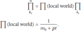
Total preferential probability is given as follows:

$$\begin{array}{cc}& {\displaystyle \prod }_{k_i}={\displaystyle \prod }_{k_i}+{\displaystyle \prod }_{c_i}.\end{array}$$

(6)

In [12], authors have considered the expenditure of energy in the process of linking nodes together. The disadvantage is that the energy in a cluster node will be exhausted in only few rounds if self-organization is allowed. In fact, the energy consumption will be relatively low, if only $k_{\text{max\_}i}$ is considered to be the limit for a cluster node to connect to others randomly.

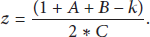
Antipreferential Attachment. Let us consider a parameter z called the deletion rate or antipreferential attachment factor, which is defined as the rate of links removed divided by the rate of links added. It is observed that lesser the energy of the node, the more will be the probability of it being deleted. Let this probability be denoted as ${\prod }_{}^{\ast }\left(k_i\right)$ .

For the outgoing cluster nodes, we have

$$\begin{array}{cc}& {\displaystyle \prod }^{\ast }\left(k_i\right)\approx \frac{\mathrm{1}}{m_{\mathrm{0}}+p\ast t}.\end{array}$$

(7)

For the outgoing normal nodes, we have

$$\begin{array}{cc}& {\displaystyle \prod }^{\ast }\left(c_i\right)\approx \frac{\mathrm{1}}{m_{\mathrm{0}}+\left(\mathrm{1}-p\right)\ast t}.\end{array}$$

(8)

So the total antipreferential probability is given as follows:

$$\begin{array}{cc}& {\displaystyle \prod }^{\ast }\left(k_i\right)+{\displaystyle \prod }^{\ast }\left(c_i\right)={\displaystyle \prod }_{k_i}^{\ast }\\ {\displaystyle \prod }_{k_i}^{\ast }=\frac{\left\{\left(\mathrm{2}\ast \left(m_{\mathrm{0}}/t\right)\right)+\mathrm{1}\right\}}{t\ast \left(m_{\mathrm{0}}/t+p\right)\ast \left(m_{\mathrm{0}}/t+\mathrm{1}-p\right)}.\end{array}$$

(9)

The antipreferential removal mechanism is more reasonable for deleting links that are antiparallel with the preferential connection. It is also consistent with the functioning of clustering algorithms that runs in rounds in wireless sensor networks. The wireless nodes that do not have enough energy, that is, the dead nodes, are to be removed from the system. Thus, antipreferential removal phenomenon is reasonable for clustering algorithms.

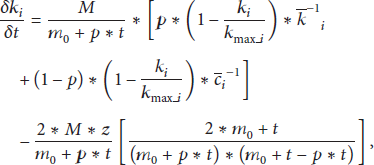
Using mean field theory [9, 13] a qualitative analysis of dynamic characterization of a wireless sensor network can be given. By the mean-field theory, the preferential and nonpreferential attachment may be combined in the following differential equation:

$$\begin{array}{cc}& \frac{\delta k_i}{\delta t}=M{\displaystyle \prod }_{k_i}^u-M\ast z\left[{\displaystyle \prod }_{k_i}^{\ast }+{\displaystyle \sum }_{j\in \mathrm{l}\mathrm{i}\mathrm{n}\mathrm{k}\mathrm{e}\mathrm{d}}{\displaystyle \prod }_{k_i}^{\ast }{k}_j^{-\mathrm{1}}{\displaystyle \prod }_{k_i}^{\ast }\right].\end{array}$$

(10)

From Li-Chen model we have

$$\begin{array}{cc}& {\displaystyle \prod }_{k_i}^u={\displaystyle \prod }\left(\text{local world}\right){\displaystyle \prod }_{k_i}\\ {\displaystyle \prod }\left(\text{local world}\right)=\frac{\mathrm{1}}{m_{\mathrm{0}}+pt}.\end{array}$$

(11)

For a single node in local world

$$\begin{array}{cc}& {\displaystyle \prod }_{k_i}^u=\frac{\mathrm{1}}{m_{\mathrm{0}}+pt}\left[{\displaystyle \prod }_{k_i}+{\displaystyle \prod }_{c_i}\right]\end{array}$$

(12)

$\begin{array}{l}\frac{\delta k_i}{\delta t}=\frac{M}{m_{\mathrm{0}}+p\ast t}\ast {\displaystyle \prod }_{k_i}\\ -\frac{M\ast z}{m_{\mathrm{0}}+p\ast t}\left[{\displaystyle \prod }_{k_i}^{\ast }+{\displaystyle \sum }_{j\in \mathrm{l}\mathrm{i}\mathrm{n}\mathrm{k}\mathrm{e}\mathrm{d}\left(i\right)}^{}{\displaystyle \prod }_{k_j}^{\ast }{k}_i^{-\mathrm{1}}{\displaystyle \prod }_{k_i}^{\ast }\right].\end{array}$

(13)

By mean field theory,

$$\begin{array}{cc}& {\displaystyle \sum }_{j\in \mathrm{l}\mathrm{i}\mathrm{n}\mathrm{k}\mathrm{e}\mathrm{d}\left(i\right)}{\displaystyle \prod }_{k_j}^{\ast }{k}_j^{-\mathrm{1}}\approx \mathrm{1}.\end{array}$$

(14)

Therefore the above equation can be rewritten as

$$\begin{array}{cc}& \frac{\delta k_j}{\delta t}=\frac{M}{m_{\mathrm{0}}+p\ast t}\ast {\displaystyle \prod }_k-\frac{M\ast z}{m_{\mathrm{0}}+p\ast t}\left[{\displaystyle \prod }_k^{\ast }+{\displaystyle \prod }_k^{\ast }\right].\end{array}$$

(15)

Using (4), (5), and (6) we have

$$\begin{array}{l}\frac{\delta k_i}{\delta t}=\frac{M}{m_0+p*t}*[p*\left(1-\frac{k_i}{k_{max\_i}}\right)*{\bar{k}}_i^1\hfill \\ \hspace{0.17em}\hspace{0.17em}\hspace{0.17em}+(1-p)*\left(1-\frac{k_i}{k_{max\_i}}\right)*{\bar{c}}_i^{-1}]\hfill \\ \hspace{0.17em}\hspace{0.17em}\hspace{0.17em}-\frac{2*M*z}{m_0+p*t}\left[\frac{2*m_0+t}{(m_0+p*t)*(m_0+t-p*t)}\right],\hfill \end{array}$$

(16)

where

$$\begin{array}{cc}& \frac{\mathrm{1}}{\overline{k_i}}=\frac{k_i}{{\sum }_i{k}_i},\\ \frac{\mathrm{1}}{\overline{c_i}}=\frac{c_i}{{\sum }_i{c}_i}.\end{array}$$

(17)

3.1. Analysis of the Dynamic Equation

3.1.1. Case I

If $z=0$ , $M=1$ ; that is, the new node selects node unless it reaches k. Moreover, the preferential attachment mechanism does not work. The rate of growth of $k_i$ is as

$$\begin{array}{cc}& \frac{\delta k_i}{\delta t}=\frac{\mathrm{1}}{m_{\mathrm{0}}+p\ast t}.\end{array}$$

(18)

The denominator of the above expression is the number of cluster nodes at time t.

3.1.2. Case II

If $M=m_0+p\ast t$ , this means that the local world is the whole network

$$\begin{array}{l}\frac{\delta k}{\delta t}\\ =p\ast \left(\mathrm{1}-\frac{k_i}{k_{\text{max\_}i}}\right)\ast \stackrel{̄}{{k^{-\mathrm{1}}}_i}+\left(\mathrm{1}-p\right)\ast \left(\mathrm{1}-\frac{k_i}{k_{\text{max\_}i}}\right)\\ \ast \overline{{c_i}^{-\mathrm{1}}}\\ -\frac{\mathrm{2}\ast M\ast z}{m_{\mathrm{0}}+p\ast t}\left[\frac{\mathrm{2}\ast m_{\mathrm{0}}+t}{\left(m_{\mathrm{0}}+p\ast t\right)\ast \left(m_{\mathrm{0}}+t-p\ast t\right)}\right].\end{array}$$

(19)

In a network, the degrees $k_i$ of most of the nodes are much smaller than their maximum $k_{\text{max\_}i}$ ; thus, we obtain the following formula:

$$\begin{array}{cc}& \mathrm{1}-\frac{k_i}{k_{\text{max\_}i}}\approx \mathrm{1}.\end{array}$$

(20)

Putting the value of (20) in (19) we have

$$\begin{array}{l}\frac{\delta k_j}{\delta t}\\ =p\ast \frac{k_i}{{\sum }_i{k}_i}+\left(\mathrm{1}-p\right)\ast \frac{c_i}{{\sum }_i{c}_i}\\ -\frac{\mathrm{2}\ast M\ast z}{m_{\mathrm{0}}+p\ast t}\left[\frac{\mathrm{2}\ast m_{\mathrm{0}}+t}{\left(m_{\mathrm{0}}+p\ast t\right)\ast \left(m_{\mathrm{0}}+t-p\ast t\right)}\right].\end{array}$$

(21)

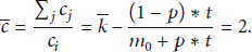
By definition

$$\begin{array}{l}\bar{k}=\frac{{\sum }_j{k}_j}{k_i}\\ \overline{k_{}}=\frac{\text{total\_degree\_of\_node\_universe}}{\text{total\_degree\_of\_nodes\_local-world}}\\ =\frac{m_{\mathrm{0}}+p\ast t+N}{m_{\mathrm{0}}+p\ast t}=\frac{m_{\mathrm{0}}+p\ast t+m_{\mathrm{0}}+t}{m_{\mathrm{0}}+p\ast t}.\end{array}$$

(22)

Therefore,

$$\begin{array}{cc}& \bar{k}=\frac{\mathrm{2}\ast m_{\mathrm{0}}+t+p\ast t}{m_{\mathrm{0}}+p\ast t}.\end{array}$$

(23)

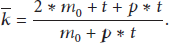
Similarly, we have for $c_i$

$$\begin{array}{cc}& \bar{c}=\frac{{\sum }_j{c}_j}{c_i}=\bar{k}-\frac{\left(\mathrm{1}-p\right)\ast t}{m_{\mathrm{0}}+p\ast t}=\mathrm{2}.\end{array}$$

(24)

As the cluster node will have one such node attached to itself the status of that node is either another cluster head or normal head hence the count value of $\bar{c}$ is 2.

Equations (21) and (23) are used to find the values of $\bar{c}$ and $\bar{k}$ .

Finally the following equation is formed after substituting the values of ${\sum }_j{c}_j$ and ${\sum }_j{k}_j$ in (21). Consider

$$\begin{array}{l}\frac{\delta k}{\delta t}=\frac{p\ast k_i}{\mathrm{2}\ast m_{\mathrm{0}}+p\ast t+t}+\left(\mathrm{1}-p\right)\\ \ast \frac{c_i}{\mathrm{2}\ast \left(m_{\mathrm{0}}+p\ast t\right)}\\ -\frac{\mathrm{2}\ast z\ast \left(\mathrm{2}\ast m_{\mathrm{0}}+t\right)}{\left(m_{\mathrm{0}}+p\ast t\right)\ast \left(m_{\mathrm{0}}+t-p\ast t\right)}.\end{array}$$

(25)

At t tends to infinity, $m_0$ tends to 0. Consider

$$\begin{array}{l}\frac{\delta k}{\delta t}=\frac{p\ast k_i}{p\ast t+t}+\left(\mathrm{1}-p\right)\ast \frac{c_i}{\mathrm{2}\ast p\ast t}\\ -\frac{\mathrm{2}\ast z\ast t}{p\ast t\ast \left(t-p\ast t\right)}.\end{array}$$

(26)

Reducing the above equation by assuming $A=p/1+p$ ,   $B=1-p/p$ , and $C=1/p\ast (p-1)$ and $c_i=2$

$$\begin{array}{cc}& \frac{\delta k}{\delta t}=\frac{A\ast k_i}{t}+\frac{B}{t}-\frac{\mathrm{2}\ast z\ast C}{t},\end{array}$$

(27)

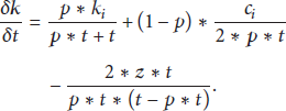
with initial conditions given as $k_i(t_i)=1$ .

By integration, we have the solution as

$$\begin{array}{cc}& \frac{t}{t_i}={\left(\frac{k\left(t\right)\ast A+B-\mathrm{2}\ast z\ast C}{A+B-\mathrm{2}\ast z\ast C}\right)}^{\mathrm{1}/A}.\end{array}$$

(28)

Moreover, to find the degree distribution $P(k)$ , that is, the probability that a node has k edges), we first calculate the cumulative probability $P[k_i(t)<k]$ . Suppose that the node enters into the network at equal time intervals. We define the probability density $t_i$ as follows:

$$\begin{array}{cc}& P\left(t\right)=\frac{\mathrm{1}}{m_{\mathrm{0}}+t}.\end{array}$$

(29)

So $P[k_i(t)<k]$ has the following form:

$$\begin{array}{cc}& \left(\mathrm{1}-{\frac{t}{t+m_{\mathrm{0}}}\left(\frac{k\ast A+B-\mathrm{2}\ast z\ast C}{A+B-\mathrm{2}\ast z\ast C}\right)}^{\mathrm{1}/A}\right).\end{array}$$

(30)

Hence, the degree distribution $P(k)$ can be obtained:

$$\begin{array}{l}\frac{\partial }{\partial t}\left(\mathrm{1}-{\frac{t}{t+m_{\mathrm{0}}}\left(\frac{k\ast A+B-\mathrm{2}\ast z\ast C}{A+B-\mathrm{2}\ast z\ast C}\right)}^{\mathrm{1}/A}\right)\\ =\frac{t}{\left(t+m_{\mathrm{0}}\right)}{\left(A+B-\mathrm{2}C\right)}^{\mathrm{1}/A}\\ ·{\left(A\ast k+B-\mathrm{2}\ast z\ast C\right)}^{-\mathrm{1}-\mathrm{1}/A}\\ \approx {\left(A+B-\mathrm{2}\ast C\right)}^{\mathrm{1}/A}\\ \ast {\left(k\ast A+B-\mathrm{2}\ast z\ast C\right)}^{-\mathrm{1}/A-\mathrm{1}}.\end{array}$$

(31)

Equation (31) denotes the degree distribution function to understand the dynamics of clustering algorithms. Putting back the values of A, B, and C we have the distribution function as the degree distribution $P(k)$ . The probability that a node has k edges is

$$\begin{array}{l}P(k)\approx {\left(\frac{p}{p-1}+\frac{1-p}{p}-\frac{2*z}{p*(1-p)}\right)}^{(1+p)/p}*(k\hfill \\ {\hspace{0.17em}\hspace{0.17em}\hspace{0.17em}\hspace{0.17em}\hspace{0.17em}\hspace{0.17em}*\frac{p}{1+p}+\frac{1-p}{p}-2*\frac{z}{p*(1-p)})}^{(-2*p-1)/p}.\hfill \end{array}$$

(32)

Next, the value of z is computed that maximizes (32). Consider

$$\begin{array}{cc}& \frac{dP\left(k\right)}{dz}=\mathrm{0}.\end{array}$$

(33)

By solving (33) we obtain the value of z as

$$\begin{array}{cc}& z=\frac{\left(\mathrm{1}+A+B-k\right)}{\mathrm{2}\ast C}.\end{array}$$

(34)

Anti preferential attachment means that the node may not like to have a particular node as its neighbor, but in this case of sensor networks no such phenomenon is observed, hence we can state that the anti preferential attachment in this particular case tends to zero during the evolution process.

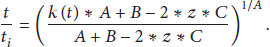
By setting the value of z to zero, we have the following relation

$$\begin{array}{cc}& p=\frac{\mathrm{1}}{\mathrm{2}}\left[{\left(\frac{k+\mathrm{3}}{k-\mathrm{1}}\right)}^{\mathrm{0.5}}-\mathrm{1}\right].\end{array}$$

(35)

Equation (35) states the probability of clustering when the antipreferential attachment factor z is zero.

4. Analysis of Topology Control Algorithms

In this section, we have carried out simulation of three localized topology control protocols, namely, A3, Simple tree Protocol, and CDS Rule K. Simulation was carried using the Atarraya [14] simulator. Total number of nodes was 100, 200, 300, and 500, respectively, and they were tested for A3, Simple Tree Protocol, and CDS Rule K. The output was recorded for average degree of nodes, k, for three protocols mentioned earlier.

Figure 2 shows an example of clustering and computation of average k value.

Figure 2

Clustering as obtained by running simple tree protocol in a network of 100 nodes.

Figure 2 shows the cluster heads in red circles with which normal nodes are attached. Taking the number of all the neighboring nodes of every cluster heads and dividing by the number of cluster heads we obtain the average value of k. By similar procedure we have obtained the average value of k for different number of nodes.

We have also carried out simulation study using simple tree protocol for different number of nodes. The number of clusters obtained using theoretical calculation (35) is compared against the number of clusters obtained using simulation study, which is presented in Table 1.

Table 1

N	k	p	$$n(T)=p\ast N$$	$$n(E)$$
100	3	0.366	37	40
200	3	0.366	73	71
300	4	0.263	79	71
400	4	0.263	105	96
500	4	0.263	132	130

N = number of nodes, k = number of neighbors, p = probability of selecting a cluster head (35), $$n(T)$$ = theoretically calculated number of clusters, and $$n(E)$$ = experimentally calculated number of clusters.

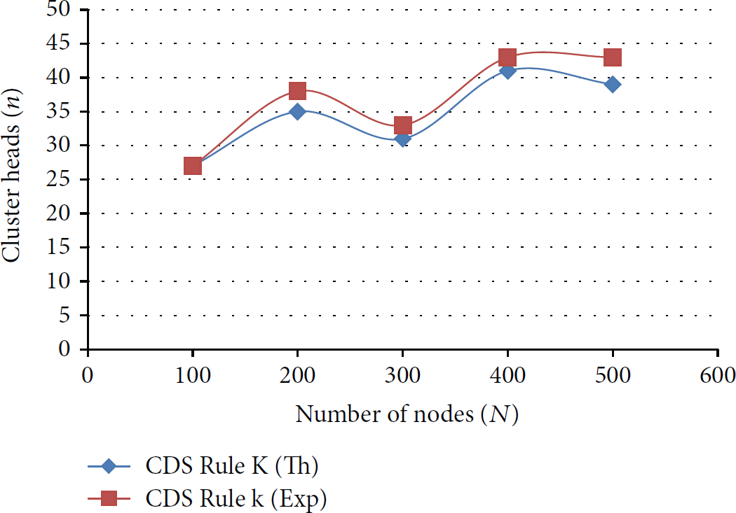
Similar simulation study was also carried out using CDS-Rule k Protocol for different number of nodes. The number of clusters obtained using theoretical calculation (35) is compared against the number of clusters obtained using simulation study, which is presented in Table 2.

Table 2

N	k	p	$$n\left(T\right)=p\ast N$$	$$n(E)$$
100	4	0.264	27	27
200	6	0.171	35	38
300	10	0.101	31	33
400	10	0.101	41	43
500	13	0.077	39	43

N = number of nodes, k = number of neighbors, p = probability of selecting a cluster head (35), $$n(T)$$ = theoretically calculated number of clusters, and $$n(E)$$ = experimentally calculated number of clusters.

Similar simulation study was also carried out using A3 Protocol for different number of nodes. The number of clusters obtained using theoretical calculation (35) is compared against the number of clusters obtained using simulation study, which is presented in Table 3.

Table 3

N	k	p	$$n(T)=p\ast N$$	$$n(E)$$
100	4	0.263	27	34
200	6	0.171	35	40
300	8	0.126	38	49
400	10	0.101	41	48
500	12	0.083	42	46

N = number of nodes, k = number of neighbors, p = probability of selecting a cluster head (35), $$n(T)$$ = theoretically calculated number of clusters, and $$n(E)$$ = experimentally calculated number of clusters.

4.1. Discussion on A3 and Simple Tree Protocol

Next, we plot the theoretically calculated number of clusters and experimentally calculated number of clusters as shown in Tables 1 and 3 for A3 and simple tree protocols.

We observe the following.

• (1)

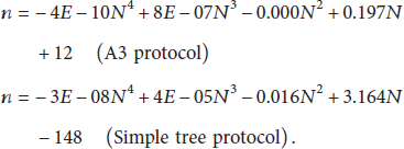
In A3 and Simple Tree protocols, the curves for theoretically calculated number of clusters and experimentally calculated number of clusters follow fourth degree equation. The trend line polynomial options of MS Excel have been used to study the degree of curve fit of the curves to obtain the following polynomials:

$$\begin{array}{ll}& n=-\mathrm{4}E-\mathrm{10}{N}^{\mathrm{4}}+\mathrm{8}E-\mathrm{07}{N}^{\mathrm{3}}-\mathrm{0.000}{N}^{\mathrm{2}}+\mathrm{0.197}N\\ +\mathrm{12}\left(\text{A3\hspace{0.17em}\hspace{0.17em}protocol}\right)\\ n=-\mathrm{3}E-\mathrm{08}{N}^{\mathrm{4}}+\mathrm{4}E-\mathrm{05}{N}^{\mathrm{3}}-\mathrm{0.016}{N}^{\mathrm{2}}+\mathrm{3.164}N\\ -\mathrm{148}\left(\text{Simple\hspace{0.17em}\hspace{0.17em}tree\hspace{0.17em}\hspace{0.17em}protocol}\right).\end{array}$$

(36)

(2)

In Figure 3, there is gap between the theoretical and experimental curves in case of A3 and simple tree protocol. This may be attributed due to the fact that A3 (approximate CDS) only preserves 1-connectivity whereas the simple tree protocol has multiple connectivity. So, A3 protocol requires less energy to construct the tree as compared to spanning tree which confirms to the experimental results.

Figure 3

Number of nodes versus number of cluster heads in simple tree protocol and A3 protocol.

4.2. Discussion on CDS Rule K

Consider (34) which is mentioned in the following:

$$\begin{array}{cc}& z=\frac{\left(\mathrm{1}+A+B-k\right)}{\mathrm{2}\ast C},\end{array}$$

(37)

where A, B, C, k, and z have been defined previously.

Table 4 enumerates the value of z for various values of k corresponding to different number of nodes in the network.

Table 4

Value of z for different k values in networks of different sizes.

Nodes collection (N)	k	Maxima ( $$p,z$$ )	Minima ( $$p,z$$ )
100	4	(0.626, 0.23618)	(0, −0.5) (1, 0)
200	6	(0.580, 0.476089)	(0, −0.5) (1, 0)
300	10	(0.54646, 0.968648)	(0, −0.5) (1, 0)
400	10	(0.54646, 0.968648)	(0, −0.5) (1, 0)
500	13	(0.53531, 1.3411)	(0, −0.5) (1, 0)

From the results of Table 2 we obtain Figure 4.

Figure 4

Total number of nodes $(N)$ versus number of cluster heads in CDS-Rule k algorithm.

In Table 4, the maximum value of z corresponds to a probability value 0.5 which indicates that the clusters have dissociated into one cluster head and one normal node which ideally predicts the case when the energy of the nodes has drained out.

In Figure 4, it can be seen that the mechanics of clustering in CDS-Rule K is in accordance to the assumptions considered while deducing the distribution function using mean field theory. Unlike A3 and Simple tree protocol, CDS-Rule K also exhibits a relation of degree 4 as shown ( $n=-2E-08N^4+3E-05N^3-0.012N^2+2.085N-87$ ). The linear graph as shown in Figure 4 represents the situation when the value of z is min. This graph is linear due to constant value of p (0.5 here) where other graphs were drawn on constant z (0 here).

Above experimental results lead us to the following explanation of the antipreferential factor z.

The antipreferential factor can have three distinct values.

• (a)

When $z=0$ then the effective degree of nodes is equal to the analytically obtained degree of a node. Here the number of cluster heads formed will be optimal.

(b)

When $z>0$ then a node will have fewer connections available. Here the number of cluster heads will be higher.

(c)

When $z<0$ then a node will have less connectivity. Here the number of cluster heads will be highest as the result will lead to dissociation.

5. Conclusions

In this paper, we have tried to provide a framework to formally model tree based clustering algorithms in a WSN. Based on the formalism, we have theoretically calculated some parameters such as number of cluster heads and average number of degree for a given algorithm. The theoretical results tally with results obtained by simulation studies. We have introduced a factor called z in network evolution model. It seems that the z factor has an impact on functioning of these protocols. We keep that study as a future exercise. The study at the current stage is more suitable for modeling tree based clustering algorithms that work on the top of connected dominating set construction. Algorithms that are based on more parameters have to be modeled appropriately in the framework before application.

In recent papers energy distribution has been considered in network evolution model for wireless sensor networks. But, so far, the framework of network evolution model has not been used to capture the characteristics of clustering algorithms.