A Hybrid Localization Approach in 3D Wireless Sensor Network

Abstract

Location information acquisition is crucial for many wireless sensor network (WSN) applications. While existing localization approaches mainly focus on 2D plane, the emerging 3D localization brings WSNs closer to reality with much enhanced accuracy. Two types of 3D localization algorithms are mainly used in localization application: the range-based localization and the range-free localization. The range-based localization algorithm has strict requirements on hardware and therefore is costly to implement in practice. The range-free localization algorithm reduces the hardware cost but at the expense of low localization accuracy. On addressing the shortage of both algorithms, in this paper, we develop a novel hybrid localization scheme, which utilizes the range-based attribute RSSI and the range-free attribute hopsize, to achieve accurate yet low-cost 3D localization. As anchor node deployment strategy plays an important role in improving the localization accuracy, an anchor node configuration scheme is also developed in this work by utilizing the MIS (maximal independent set) of a network. With proper anchor node configuration and propagation model selection, using simulations, we show that our proposed algorithm improves the localization accuracy by 38.9% compared with 3D DV-HOP and 52.7% compared with 3D centroid.

1. Introduction

Knowing the accurate position of a certain object is crucial for many context aware applications in wireless sensor networks (WSNs), such as target tracking, geographic routing, and even energy management [1–3]. Therefore, many localization algorithms and related systems are proposed by leveraging different techniques towards the accurate and practical localization in WSNs. A detailed survey on location, localization, and localizability in WSNs can be found in [4].

The earliest attempt for 3D space localization is based on trilateration. The position of an unknown node can be determined based on the known coordinates of four reference nodes which are not in the same plane and the precise distances to them. Although absolutely accurate distances are generally unprocurable in practice, the Euclidean distance between two nodes in a wireless sensor network can be estimated by their shortest path with the per hop distance measured by received signal strength indicator (RSSI) or time difference of arrival (TDOA) or simply assumed as a constant.

With regard to the mechanisms used for estimating location in 3D environment, existing literature can be mainly grouped into two categories: range-based [5, 6] and range-free [7, 8] algorithms. The range-based algorithm is featured by the relatively high hardware requirements. Landscape-3D [9] is the first robust 3D range-based localization algorithm, in which the localization accuracy heavily relies on the expensive mobile beacon. The range-free algorithms are normally using connectivity information [10, 11] only to achieve localization, such as centralized algorithms 3D multidimensional scaling-map (3D MDS-MAP) [12], 3D DV-HOP [13], and 3D centroid [14], which are modified from 2D-plane scenarios. These approaches achieve coarse-grained localization at the cost of high computational complexity.

Recently, there has been growing interest in localization protocols that utilize the network topology characteristic [15]. CATL [12] splits the whole rugged network into several subsections and then carries out the localization in each subnetwork. It optimized the anchor node configuration to improve localization accuracy. Considering the node deployment strategy [16], the 3D range-free techniques always have strict network connectivity requirements, making them unsuitable for the large scale sensor networks.

In this paper, we propose a hybrid localization approach to overcome the shortage of range-free and range-based algorithms, by combining RSSI value and hop distance for 3D WSN localization, henceforth referred to as 3D-RDH algorithm. Our proposal utilizes the range-free technique by blending the RSS information under a proper selected model. As RSS data can be easily collected with current off-the-shelf equipment, it is the basis of many popular techniques for inferring the relative positions of the nodes in a WSN, whereas DV-HOP uses the network connectivity information to estimate unknown node location, especially considering the connectivity of 3D sensor network much higher than the 2D case. Inspired by the idea of virtual backbone [17] of a wireless sensor network, we place anchor nodes in the network based on maximum independent set (MIS) of the network to further improve the localization accuracy. Experimental results show that our proposal can achieve much higher localization accuracy compared with existing proposals.

Towards the accurate localization, a key is to identify the hybrid approach of localization and extract a graph of the network for anchor node configuration during deployment, which is, however, often impractical to achieve in reality. This is attributed to many fundamental engineering challenges as follows. Firstly, there is a lack of understanding of selecting proper localization techniques. Secondly, there are available schemes from the computer graphics community to find an independent set. They target high connectivity and low cost. The network is discrete and a sensor node can only obtain local information via message exchanges. A low communication complexity scheme to identify a MIS is necessarily required considering the limited resource of each sensor node. Lastly, since an independent set is discrete and arbitrary, it is not easy to clearly specify which nodes in a MIS can be selected as the anchor nodes. In this paper, we address the aforementioned challenges in one framework.

Our key contributions can be summarized in three key points.

• (i)

We develop an improved maximum independent set construction algorithm for a WSN considering communication complexity. We also prove that nodes chosen from a MIS are sufficient for anchor nodes configuration.

(ii)

A hybrid localization scheme is proposed to achieve 3D localization, which utilizes the range-based attribute RSSI to correct the range-free attribute hopsize.

(iii)

Via high fidelity simulations, we show that 3D-RDH algorithm can achieve much higher localization accuracy compared with other existing localization approaches in 3D environment.

The remainder of this paper is organized as follows. Section 2 outlines the previous algorithms carried out on DV-HOP localization and some problems of this traditional algorithm. Then the 3D-RDH algorithm is introduced in Section 3; it consists of four parts: anchor nodes deployment, RSSI model selection, the hop distance revision, and the whole procedure of the algorithm. Section 4 presents a description of the simulation scenarios and results. Algorithm performance evaluation in terms of accuracy and network connectivity is also discussed in this part. Finally, the conclusion and future work are discussed in Section 5.

2. Related Work

2.1. DV-HOP Algorithm

DV-HOP algorithm [18] is proposed by Niculescu and Nath in the Navigate project. It can be divided into three steps. Firstly, each anchor node broadcasts a beacon to be flooded throughout the network. Then all nodes can obtain the shortest hop count away from each anchor. Next, each anchor node calculates its own average single hopsize based on the following equation,

$$\begin{array}{cc}& {\text{Hopsize}}_m=\frac{\sum ‍\sqrt{{\left(x_m-x_n\right)}^{\mathrm{2}}+{\left(y_m-y_n\right)}^{\mathrm{2}}}}{\sum ‍h_n},\end{array}$$

(1)

and then broadcasts it to the whole network. In this formula, $(x_m,y_m)$ and $(x_n,y_n)$ are two different anchor nodes' locations, and $h_n$ is the hop count from anchor n to m. The unknown nodes then work out the estimated physical distance between themselves and the anchor nodes based on the average hopsize. Finally, the unknown node can estimate its location by using triangulation or maximum likelihood estimates.

2.2. Problems of DV-HOP Algorithm in Real Practice

DV-HOP algorithm provides an effective localization in large scale WSNs. However, it still faces several challenges. First, the approach of accumulating the hop count is rough. DV-HOP algorithm views the hop count between arbitrary two neighboring nodes as 1, regardless of the real distance between them. Besides that, the average hopsize calculated from the rough hop count can lead to an inaccurate estimated distance between an anchor node and an unknown node. The estimated coordinates of unknown nodes may also be incorrect.

To address these challenges, there are many algorithms proposed to improve the DV-HOP algorithm in 2D environment. Literature [19] requires the anchor nodes deploying at the boundary of the network, so that the average hop distance can be improved, while literature [20] focuses on the range correction. The improved algorithm proposed in [20] enhances the localization accuracy by calculating the distance between the unknown node and anchor nodes based on multiplying the distance correction factor.

These algorithms mentioned above improve the position accuracy at the expense of localization rate and computational complexity. For example, although deploying the anchor nodes in the boundary of the network can improve the average single hop distance accuracy, the localization rate can be decreased. More importantly, although correcting the average hop distance by correction coefficient can improve the accuracy, the approach of elevating the accuracy through loop calculation may increase the computational overhead and the time complexity.

In recent years, hybrid location techniques have attracted increasing research efforts. Literature [21] is a hybrid localization algorithm based on DV-Distance and the twice-weighted centroid in WSN. It combines two range-free schemes to achieve more precise location. This approach uses the DV-Distance localization algorithm to get the cumulative distance and the rough-estimated coordinate for calculating twice-weighted factors. This algorithm can increase location accuracy by 20% compared with traditional centroid algorithm, but its experimental environment is in an ideal environment. It is not proper for the actual WSN environment. Different from [21], literature [22] utilizes the advantages of two range-based techniques. The two widely used ranging techniques are time of arrival (TOA) using ultra-wideband (UWB) and received signal strength (RSS) using WiFi signals. This approach cannot be widely used in large scale WSNs as it involves additional hardware for each node.

2.3. Anchor Nodes Placement

Only a few studies of WSN localization are focused on the anchor nodes in 3D space. How to choose and place reference nodes plays an important role in the positioning accuracy. Literature [23] shows that localization is closely related to the placement method of anchor nodes. However, those studies are based on 2D plane only. Literature [24] proves that the placement of anchor nodes has a great impact on the location performance. It however lacks further description on how to place reference nodes in 3D environment. This paper proposes an anchor nodes placement approach based on network backbone [25, 26] and designs an anchor nodes selection algorithm in order to improve the localization accuracy under the same condition.

3. 3D-RDH Algorithm

In this section, a hybrid localization approach for 3D WSN which combines the RSS data and hop distance is presented. It improves the range-free technique DV-HOP by introducing reference RSSI value to revise the hop distance. In addition, an anchor node configuration scheme and RSSI model are discussed in the proposed algorithm.

3.1. Anchor Placement

Anchor placement plays an important role in the quality of spatial localization. Inspired by virtual backbone, we deploy our anchor nodes based on the MIS of a network. Virtual backbone of a network contains backbone nodes of the network and it is used to solve the problems such as the notorious broadcast storm problem. The virtual backbone of the network can be obtained by previous algorithm [25, 27, 28]. The configuration of anchor nodes will be identified by sampling the induced topology of a MIS in the network.

3.1.1. Preliminaries

We first introduce some important notations and concepts used in the paper as follows.

• (i)

SUG (simple undirected graph): given a simple undirected graph $G(V,E)$ , V represents the vertices of the graph and E represents the edges of the graph.

(ii)

IS (independent set): an independent set I of V is a subset of V such that $\forall u,v\in V$ , $uv\notin E$ .

(iii)

MIS (maximal independent set): an independent set $V^{\prime }$ of V is a subset of V such that $\forall u,v\in V$ , $uv\notin E$ , for $\forall u\in V\text{-}{V}^{\prime }$ , there exists a $v\in V^{\prime }$ satisfying $uv\in E$ .

(iv)

DS (dominating set): in a graph $G(V,E)$ , a dominating set D of $G(V,E)$ is a subset of V such that, for $\forall u\in V\text{-}D$ , there exists a $v\in D$ satisfying $uv\in E$ .

(v)

CDS (connected dominating set): if all nodes in DS induce a connected graph, DS is a connected dominating set.

(vi)

MCDS (minimum connected dominating set): among all connected dominating sets of V, the one with the smallest cardinality is called the minimum connected dominating set.

3.1.2. Network Model Definition

We model the wireless sensor network as a SUG (simple undirected graph) denoted as $G(V,E)$ . Here, V represents the set of sensor nodes and E represents the set of edges. An edge $uv\in E$ if and only if $u,v\in V$ and the Euclidean distance between u and v is smaller than 1 unit. Sensor nodes in SUG can communicate with each other if this distance is at most 1 unit.

3.1.3. MIS Construction

MIS is a node set, and, in this set, arbitrary two nodes are not connected and all the nodes outside the set are connected with at least one node in the MIS. MIS is frequently used as the basis of constructing a network virtual backbone as it can include as much as possible nodes which are evenly dispersed in a network. Inspired by virtual backbone, we come up with the idea that is based on MIS to choose anchor nodes. There are many existing works about MIS construction [25, 29]. For example, literature [25] constructs the backbone via algebraic connectivity and introduces a new metric, namely, connectivity efficiency, as a benchmark when constructing the backbone. In our work, we adopt the algorithms about MIS construction proposed in [29–31] and apply them in our simulation. Through literature [28], we can know that the nodes number in MIS is $\mathrm{8}\times N_{opt}+\mathrm{3}$ ; here $N_{opt}$ is the nodes number of MCDS. MCDS (minimum connected dominating set) is composed of the minimum number nodes of all CDS in a network.

To construct MIS, firstly we define several functions: color $(p)$ represents the state of node p. Color “white” indicates the initial state. Color “red” indicates that the node is in the ready state. Color “black” indicates that the node is a master. Color “gray” indicates that the node is a slave node. Message $(p)$ represents the information broadcasted by the node p, “manager,” “subordinate,” and “ready.” Node p in different states will broadcast different messages. For example, when a node becomes the master, it will broadcast “manager” information to its neighbors, while a slave node broadcasts “subordinate”; if a node receives “subordinate” information, it will become a ready node and broadcast “ready” information.

At the beginning of the construction, we will choose an arbitrary node to be the leader as the initial node or choose it by the leader election algorithm. After the election of the leader, the state transformation process of each node is shown in the following steps.

Step 1.

If node p is a leader, the leader will be directly promoted to be a master. The color of this node will be changed to black from white.

Step 2.

If an initial node p receives “manager” information from master U and the color of this node is white, then node U will be the master of p and p becomes a slave node. Node p's color will be changed to gray from white and it will broadcast “subordinate” information.

Step 3.

If an initial node p receives “subordinate” information, the node will enter the ready state and becomes a ready node. Node p's color will be changed to red from white and it will broadcast “ready” information.

Step 4.

If a node p's color is white or red and it receives the “ready” information, then the state of this node does not change and node p only records the red neighbors' information.

Step 5.

If node p's color is red, then compare all the red nodes in the network and choose the node that has the minimum ID as the next master. Change node p's color to black and its message to “managers.”

The end condition of Algorithm 1 is that there does not exist any white node in the network. Through this algorithm, several star shaped structures are produced. In each star structure, a black node as a master connects multiple grey slave nodes.

Algorithm 1: MIS construction.

begin

    input: a nodes set A consists of all nodes in the network (The serial number ID of each node is known)

    output: MIS of the network

(1)   Initialization:

(2)   the ID number of each node is known;

(3)   set all nodes' color as white;

(4)   set all nodes' message as null.

(5)   A leader node p produced by the leader election algorithm, then set:

(6)   color(p) = black; message(p) = “manager”;

(7)   for  each node q in A  do

(8)     if   $$color(q)==white$$   then

(9)         if  q receives “manager” message  then

(10)          color(q) = gray;

(11)           message(q) = “subordinate”;

(12)        if  q  receives “subordinate” message  then

(13)          color(q) = red;

(14)          message(q) = “ready”;

(15)    if   $$color(q)==red$$   then

(16)    Put q and q's neighbors whose color is red into array M;

(17)    Choose the minimum ID from all ID in M;

(18)    And find the coordinate node r to become a master;

(19)    Then set: color(r) = black;

      message(r) = “manager”;

(20)   Repeat (7–19) until there doesn't exist white node in whole network;

Lemma 1.

The size of maximum independent set in $G=(V,E)$ is at least 4 and at most $(\mathrm{8}opt+\mathrm{3})$ ; $opt$ is the size of MCDS of G in the theory.

Proof.

It can be known that the size of maximum independent set is at least 4 according to the concept of MIS. Let M be the maximum independent set of V, and let T be the corresponding spanning tree of the MCDS in the theory. Consider an arbitrary preorder traversal of T given by $v_{\mathrm{1}},v_{\mathrm{2}},v_{\mathrm{3}},\dots ,v_{opt}$ . Let $M_{\mathrm{1}}$ be the set of nodes in M that are adjacent to $v_{\mathrm{1}}$ . For any $\mathrm{2}\le i\le opt$ , let $M_i$ be the set of nodes in M that are adjacent to $v_i$ but not adjacent to $v_{\mathrm{1}},v_{\mathrm{2}},\dots ,v_{i-\mathrm{1}}$ . Then $M_{\mathrm{1}},M_{\mathrm{2}},\dots ,M_{opt}$ form a partition of M. Based on literature [32], it is clear to know that $v_{\mathrm{1}}$ can be adjacent to at most 11 independent nodes. So the following equation can be obtained:

$$\begin{array}{cc}& \left|M_{\mathrm{1}}\right|\le \mathrm{11},\\ \left|M_i\right|\le \mathrm{8}.\end{array}$$

(2)

For any $\mathrm{2}\le i\le opt$ , at least one node in $v_{\mathrm{1}},v_{\mathrm{2}},\dots ,v_{i-\mathrm{1}}$ is adjacent to $v_i$ . Therefore,

$$\begin{array}{cc}& \left|M\right|={\displaystyle \sum }_{i=\mathrm{1}}^{opt}‍\left|M_i\right|=\left|M_{\mathrm{1}}\right|\le \mathrm{11}+\mathrm{8}\left(opt-\mathrm{1}\right)=\mathrm{8}opt+\mathrm{3}.\end{array}$$

(3)

Then the size of maximum independent set in $G=(V,E)$ is at least 4 and at most ( $8opt+3$ ), $opt$ is the size of MCDS of G in the theory.

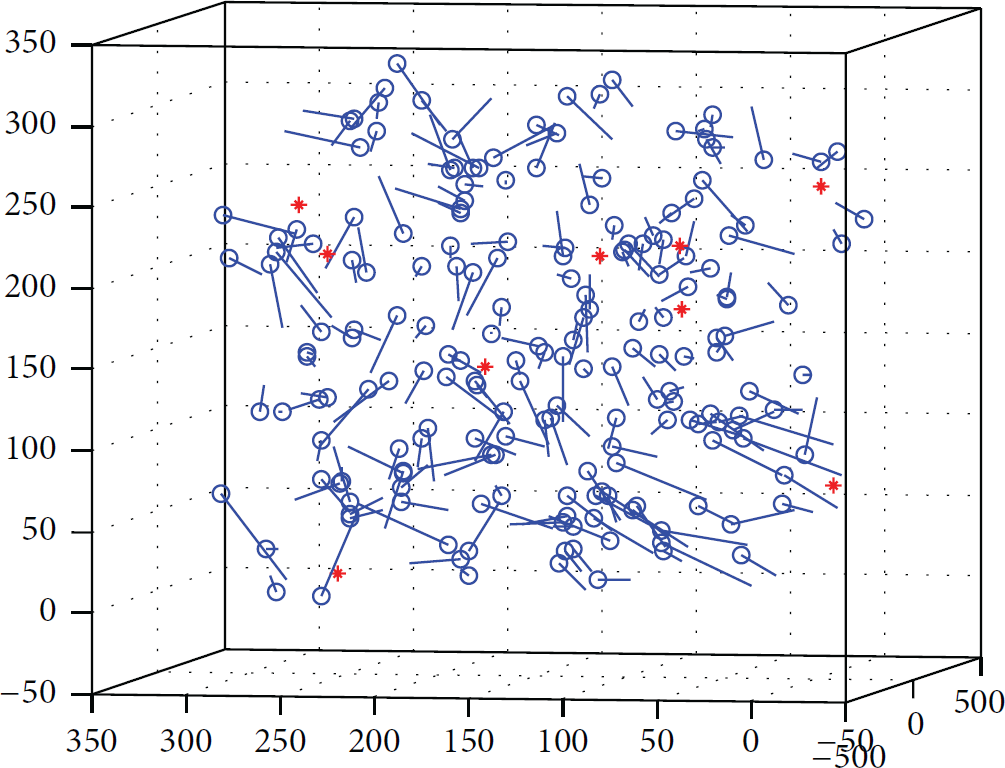
According to the process of MIS construction, for any vertex u in a maximal independent set I, the length of the shortest path from u to its closest vertex in I is either two hops or three hops. In the following MIS construction simulation, nodes are randomly distributed in an area of $\mathrm{300}\hspace{0.17em}\text{m}\times \mathrm{300}\hspace{0.17em}\text{m}$ and the communication radius of the network is set as $\mathrm{100}$  m. Figure 1 shows the simulation results of MIS construction. Figure 1(a) shows MIS construction result when the total number of sensor nodes is 150. To see the result of MIS clearly, here we only show the dominating nodes are marked as red. And Figure 1(b) shows the results of MIS construction when the total number of nodes in the network is chosen from $[\mathrm{80}\hspace{0.5em}\mathrm{100}\hspace{0.5em}\mathrm{120}\hspace{0.5em}\mathrm{140}\hspace{0.5em}\mathrm{160}\hspace{0.5em}\mathrm{180}\hspace{0.5em}\mathrm{200}]$ .

Figure 1

The simulation result of MIS construction.

From Figure 1, it can be seen that the size of MIS is more than 4, which can meet the requirement of anchor nodes. According to [33], the size of independent set in $G=(V,E)$ is at most $(\mathrm{8}opt+\mathrm{3})$ ; $opt$ is the size of MCDS of G in theory. The detailed proof is shown in [33].

3.1.4. Anchor Nodes Deployment

With established MIS of the network, we start to place the anchors. The serial number of each node in MIS can be known. Here, we mark the MIS as M. The selection approach is based on the cluster analysis. We use hop count similarity method to divide the whole nodes set to several clusters. Firstly, we generate N uniformly dispersed ( $\mathrm{4}\le N\le \mathrm{8}\times N_{opt}+\mathrm{3}$ ) nodes as seed nodes in the network region. Each node in M calculates the hop counts from N seed nodes. It will be put into cluster S when it has the shortest hop count with seed node S. For example, if we need deploy 10 anchor nodes, we generate 10 seed nodes and divide the whole MIS nodes set into 10 clusters. Next, choose a node q in ${\text{cluster}}_{\mathrm{1}}$ randomly and put q's serial number into an array B. Then find nodes that have the largest hop count with q in other clusters and record their serial number in B. According to this method find all proper nodes in each cluster. Finally we can get a certain number of nodes as a basis to deploy anchor nodes. The detail is listed as Algorithm 2.

Algorithm 2: Anchor nodes deployment.

begin

    input: a nodes set M of MIS (The serial number of each node is known)

    output: N serial number used to deploy anchor nodes

(1) Generate $$N\hspace{0.17em}\hspace{0.17em}(\mathrm{4}\le N\le \mathrm{8}\mathrm{*}{N}_{opt}+\mathrm{3})$$ uniformly dispersed nodes as seed nodes in the network region.

(2) for  each node P in M  do

(3)    calculate the hop counts from N seed nodes.

(4)    if  the hop count between P and seed node $$S_i$$ is least  then

(5)      P belongs to $$S_i$$ .

(6) Then M is divided into N cluster.

(7) Define int $$i\hspace{0.17em}\hspace{0.17em}(\mathrm{1}\le i\le N)$$ as the serial number of N cluster.

(8) Choose one node q randomly in $$cluste{r}_{\mathrm{1}}$$ and put q's serial number into array B.

(9) if   $$i<N$$   then

(10)  Find the largest hop count between q and the node r in $$cluste{r}_{i+\mathrm{1}}$$ ;

(11)  Use array B to record the node r's serial number;

(12)  i++;

(13)  for   $$i=1:N$$   do

(14)  return $$B_i$$ ;

(15)  N serial number is obtained, then return them.

3.2. RSSI Communication Propagation Model Selection

The proper propagation model selection is critical in the proposed algorithm, as it directly affects the way we calculate path loss. The path loss can reflect the distance between arbitrary two sensor nodes. Within our knowledge, the RSSI value is easily affected by the wireless signal reflection, absorption, and other noises. Figure 2 demonstrates that the increasing RSSI value can largely reflect a relative closer distance between two nodes.

Figure 2

The relationship between RSSI attenuation value and distance.

Many channel models have been proposed for outdoor and indoor environments. We group them into two categories: regular model and irregular model. In regular model, the received signal strength is represented by the difference between the emission signal strength and the transmission loss. However, in practical applications, the regular model cannot reflect the exact channel state. This is due to the fact that the propagation range of radio signals in real world will be affected by shadow effect, reflections propagation, refraction propagation, scatter propagation, propagation, diffraction propagation, and other factors, which makes the relationship between signal strength and distance difficult to determine. In view of this circumstance, several irregular models are proposed, such as DOI model and RIM model [34].

In our tests, we choose the DOI model to capture the reference RSSI value as RIM model is too sensitive to the environment. DOI (degree of irregularity) is defined as the percentage of the variation degree in the wireless communication's unit direction about the maximum path loss. DOI model is a universal wireless propagation model. The DOI model is on the basis of the following formula:

$$\begin{array}{cc}& P_R\left(d\right)=P_T-P_L\left(d_{\mathrm{0}}\right)-\mathrm{10}\eta \hspace{0.17em}{\log }_{\mathrm{10}}\frac{d}{d_{\mathrm{0}}}\times k_i.\end{array}$$

(4)

Here, $P_R(d)$ is the received signal power in dB at distance d; $P_T$ is the emission signal power; $P_L(d_{\mathrm{0}})$ is the path loss power at distance $d_{\mathrm{0}}$ ; η is the path loss exponent; d is the distance between the sending and receiving end. In the above formula, except $K_i$ , other symbolic meanings are the same as that of the regular model's formula mentioned above. And here, $K_i$ is the path loss coefficient of concordance and i is used to represent the different directions, $i\in [\mathrm{0,360}]$ . $K_i$ can be calculated according the following formula:

$$\begin{array}{cc}& K_i=\left\{\begin{array}{cc}\mathrm{1},\hfill & i=\mathrm{0};\hfill \\ K_i\pm \text{rand}\times \text{DOI},\hfill & \mathrm{0}<i<\mathrm{360}\cap i\in N,\hfill \\ \left|K_{\mathrm{0}}-K_{\mathrm{359}}\right|\le \text{DOI}.\hfill & \hfill \end{array}\right.\end{array}$$

(5)

Therefore we can calculate the different $K_i$ value from all different directions.

3.3. The Hop Distance Revision

As showed in the above introduction of the traditional DV-HOP algorithm, the hopsize is calculated based on the hop count. The hop count and hopsize are both modified in the proposed algorithm.

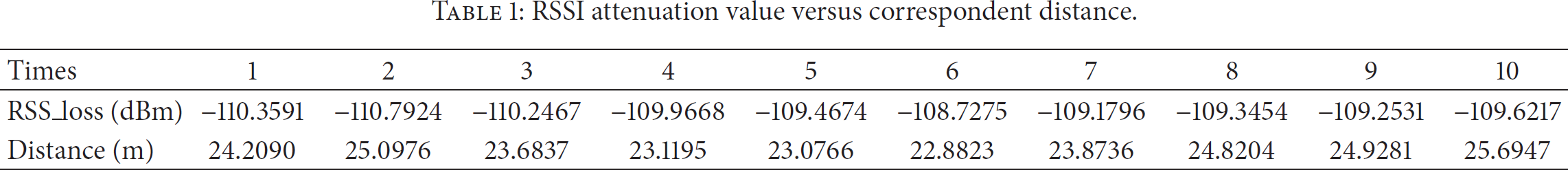
When hop count between unknown node and anchor node is 1, we use the distance calculated based on the RSSI attenuation value to replace the distance estimated by using the average single distance. As we all know, the distance estimated by RSSI attenuation value is relatively precise within the communication range. For example, as shown in Figure 3, $P_{\mathrm{1}}$ , $P_{\mathrm{2}}$ , $P_{\mathrm{3}}$ , and $P_{\mathrm{4}}$ are anchor nodes and A, B, C, D, E, and F are the unknown nodes. The real distance between 2 terminal nodes is marked as red while the RSSI value between two nodes is marked as blue number. According to the method of the traditional DV-HOP algorithm, the average single hop distance of $P_{\mathrm{2}}$ can be calculated by the following formula: ${\text{hopsize}}_{P_{\mathrm{2}}}=(\mathrm{40}+\mathrm{40}+\mathrm{40})/(\mathrm{4}+\mathrm{6}+\mathrm{5})=\mathrm{8}$ . From this, we can work out the distance between node A and the anchor node $P_{\mathrm{2}}$ to be 8, while the real distance between them is 25 m. However, if we use the RSSI attenuation value, we can get a RSSI attenuation value $-\mathrm{110.4502}$  dBm, and then using DOI model we can calculate a more precise distance value $\mathrm{25.5092}$  m, which improves the distance measurement greatly compared to traditional method. To find further evidence, several rounds of simulations were carried out to show the association between RSSI value and corresponding distance. Table 1 shows the distances with respect to relative RSSI value between anchor node $P_{\mathrm{2}}$ and node A. We set the communication radius to 30 m and the DOI (degree of irregularity) to 0.015. Then we get these measurements shown in Table 1. From these data, it is clear to see that the estimated results are closer to the real distance and they have a difference of about 2 meters.

Table 1

RSSI attenuation value versus correspondent distance.

Times	1	2	3	4	5	6	7	8	9	10
RSS_loss (dBm)	−110.3591	−110.7924	−110.2467	−109.9668	−109.4674	−108.7275	−109.1796	−109.3454	−109.2531	−109.6217
Distance (m)	24.2090	25.0976	23.6837	23.1195	23.0766	22.8823	23.8736	24.8204	24.9281	25.6947

Figure 3

The distance error.

When hop count is greater than 1, decimal counts are accumulated in the proposed algorithm. In our approach, we set the beacon of anchor nodes with the following information: ID number, location, hop counts initialized to zero, and $R_{ij}$ . Particularly, the forth term $R_{ij}$ is defined as the decimal hop count between nodes i and j. It can be calculated by the formula: $R_{ij}={\text{RSSI}}_{\text{loss}}/\text{Ref}$ . Here, “Ref” is the corresponding RSSI value to the communication radius. $R_{ij}$ represents the ratio of the RSSI attenuation value between two nodes i and j and Ref.

We can also clearly represent this method using Figure 4. Given the communication radius 30 m, we can get the “Ref” $-\mathrm{122.4880}$  dBm. Anchor node $P_1$ broadcasts beacons to the whole network and node C receives. C increases the hop count by 1 and set $R_{P_{\mathrm{1}}\text{C}}$ to $-\mathrm{90.3225}/-\mathrm{122.4880}=\mathrm{0.7374}$ . $-\mathrm{90.3225}$ is the RSSI attenuation from $P_{\mathrm{1}}$ to C. Then C broadcasts the beacon, and B receives. B also increases the hop count by 1; now the hop count between B and $P_{\mathrm{1}}$ is $\mathrm{2}$ . Besides, B set $R_{P_{\mathrm{1}}\text{B}}$ is equal to the sum of $R_{P_{\mathrm{1}}\text{C}}$ and $R_{\text{CB}}$ . It can be computed by the following formula: $R_{P_{\mathrm{1}}\text{B}}=R_{P_{\mathrm{1}}\text{C}}+R_{\text{CB}}=\mathrm{0.7374}+\mathrm{0.7963}=\mathrm{1.5337}$ . With the propagation of these beacons, the hop count and $R_{ij}$ can be obtained. With the combination of Freud's law, we can get the shortest hop count and $R_{ij}$ between two nodes of the whole network. Then the average hop distance of $P_2$ is shown by the following formula: ${\text{Hopsize}}_{P_{\mathrm{2}}}=(\mathrm{40}+\mathrm{40}+\mathrm{40})/(\mathrm{3.3065}+\mathrm{4.5901}+\mathrm{3.8019})=\mathrm{10.2577}$ .

Figure 4

The procedure of 3D-RDH algorithm.

Through the preceding calculation method, the average hop distance of $P_{\mathrm{1}}$ , $P_{\mathrm{3}}$ , and $P_{\mathrm{4}}$ can also be calculated, ${\text{Hopsize}}_{P_{\mathrm{1}}}=\mathrm{12.69}$ , ${\text{Hopsize}}_{P_{\mathrm{3}}}=\mathrm{12.82}$ , and ${\text{Hopsize}}_{P_{\mathrm{4}}}=\mathrm{11.91}$ , while the hopsize of these four anchors is separately 9.95, 8, 9.95, and 9.23 by using the traditional approach. Besides, the hop count between A and $P_{\mathrm{1}}$ , $P_{\mathrm{3}}$ , $P_{\mathrm{4}}$ can also be obtained. Using traditional method, the result is 3, 5, and 4, while using our proposed approach the result is 2.2128, 3.7379, and 2.9497. Then we can estimate the distance between the four anchor nodes and A using the following formula: ${\text{Distance}}_{\text{estimated}}=\text{Hopsize}*\text{hop}\mathrm{\hspace{0.17em}\hspace{0.17em}}\text{count}$ . We can get the estimated distance between B and the four anchors: $\text{A-}{P}_{\mathrm{1}}$ : $\mathrm{12.69}\times \mathrm{2.2128}=\mathrm{28.08}$ , $\text{A-}{P}_{\mathrm{2}}$ : 25.51 (hop count = 1), $\text{A-}{P}_{\mathrm{3}}$ : $\mathrm{12.82}\times \mathrm{3.7379}=\mathrm{47.92}$ , and $\text{A-}{P}_{\mathrm{4}}$ : $\mathrm{11.91}\times \mathrm{2.9497}=\mathrm{35.1}$ . According to the calculation result of the traditional approach, we can get the distances between A and these four anchor nodes as follows: 29.85, 8, 49.75, and 36.92. By comparing the two sets of data, it is clear to see that the previous group is closer to the actual distance.

3.4. The Procedure of 3D-RDH Algorithm

The flow chart of the proposed algorithm is shown in Figure 4. It can be described as follows.

(1) Broadcast the information of the anchor nodes: each anchor node generates and broadcasts a beacon containing its own information: ID number, location, hop count initialized to 0, and $R_{ij}$ ; here i is the ID number of the anchor node and j is its neighbor node number. When a neighbor node m receives a beacon message of anchor node P, m will increase the hop count by 1 and set the $R_{Pm}$ to the ratio of the RSSI value from P and the reference Ref. Then node m will carry on forwarding the new beacon message. When the message arrives at its neighbor node n, the hop count will be accumulated by 1, and $R_{Pn}$ can be obtained by adding $R_{Pm}$ to $R_{mn}$ . The beacon message will be passed throughout the whole network following Freud's law. In the end, the shortest hop count and $R_{ij}$ of the whole network between nodes can be calculated and recorded.

(2) Calculate the distance between the unknown and anchor nodes: with the known distance between anchor nodes, the average hop distance of each anchor node is computed. Next, for neighboring nodes of anchor nodes, the distance between them can be obtained directly through the propagation model with RSSI value. For unknown nodes with hop count ≥ 2, the distance can be calculated by the multiple of $R_{ij}$ and the average hopsize of this anchor node.

(3) Estimate the coordinates of the unknown: based on the preceding steps, the unknown can estimate its own coordinate by using maximum likelihood estimate. Suppose there are $n\hspace{0.17em}\hspace{0.17em}(n\ge \mathrm{4})$ reference nodes in 3D network and their coordinates are $(x_1,y_1,z_1),(x_2,y_2,z_2),(x_3,y_3,z_3),\dots ,(x_n,y_n,z_n)$ separately, the coordinate of unknown node P is $(x,y,z)$ , and the distance between P and m reference nodes $(m\le n)$ that have connectivity with P is $d_{\mathrm{1}},d_{\mathrm{2}},\dots ,d_m$ . Then the following equation set can be obtained based on space distance formula between two nodes:

$$\begin{array}{l}{\left(x_{\mathrm{1}}-x\right)}^{\mathrm{2}}+{\left(y_{\mathrm{1}}-y\right)}^{\mathrm{2}}+{\left(z_{\mathrm{1}}-z\right)}^{\mathrm{2}}=d_{\mathrm{1}}\\ {\left(x_{\mathrm{2}}-x\right)}^{\mathrm{2}}+{\left(y_{\mathrm{2}}-y\right)}^{\mathrm{2}}+{\left(z_{\mathrm{2}}-z\right)}^{\mathrm{2}}=d_{\mathrm{2}}\\ {\left(x_{\mathrm{3}}-x\right)}^{\mathrm{2}}+{\left(y_{\mathrm{3}}-y\right)}^{\mathrm{2}}+{\left(z_{\mathrm{3}}-z\right)}^{\mathrm{2}}=d_{\mathrm{3}}\\ ⋮\\ {\left(x_m-x\right)}^{\mathrm{2}}+{\left(y_m-y\right)}^{\mathrm{2}}+{\left(z_m-z\right)}^{\mathrm{2}}=d_m.\end{array}$$

(6)

After subtracting the last formula separately, the previous $m-\mathrm{1}$ formula can be simplified as the following formula set:

$$\begin{array}{l}\mathrm{2}\left(x_{\mathrm{1}}-x_m\right)x+\mathrm{2}\left(y_{\mathrm{1}}-y_m\right)y+\mathrm{2}\left(z_{\mathrm{1}}-z_m\right)z\\ \hspace{1em}=\left(x_{\mathrm{1}}^{\mathrm{2}}+y_{\mathrm{1}}^{\mathrm{2}}+z_{\mathrm{1}}^{\mathrm{2}}\right)-\left(x_m^{\mathrm{2}}+y_m^{\mathrm{2}}+z_m^{\mathrm{2}}\right)-\left(d_{\mathrm{1}}^{\mathrm{2}}-d_m^{\mathrm{2}}\right);\\ \mathrm{2}\left(x_{\mathrm{2}}-x_m\right)x+\mathrm{2}\left(y_{\mathrm{2}}-y_m\right)y+\mathrm{2}\left(z_{\mathrm{2}}-z_m\right)z\\ \hspace{1em}=\left(x_{\mathrm{2}}^{\mathrm{2}}+y_{\mathrm{2}}^{\mathrm{2}}+z_{\mathrm{2}}^{\mathrm{2}}\right)-\left(x_m^{\mathrm{2}}+y_m^{\mathrm{2}}+z_m^{\mathrm{2}}\right)-\left(d_{\mathrm{2}}^{\mathrm{2}}-d_m^{\mathrm{2}}\right);\\ \hspace{1em}\hspace{1em}\hspace{1em}\hspace{1em}\hspace{1em}\hspace{1em}\hspace{1em}\hspace{1em}\hspace{1em}⋮\\ \mathrm{2}\left(x_{m-\mathrm{1}}-x_m\right)x+\mathrm{2}\left(y_{m-\mathrm{1}}-y_m\right)y+\mathrm{2}\left(z_{m-\mathrm{1}}-z_m\right)z\\ \hspace{1em}=\left(x_{m-\mathrm{1}}^{\mathrm{2}}+y_{m-\mathrm{1}}^{\mathrm{2}}+z_{m-\mathrm{1}}^{\mathrm{2}}\right)\\ \hspace{1em}\hspace{1em}-\left(x_m^{\mathrm{2}}+y_m^{\mathrm{2}}+z_m^{\mathrm{2}}\right)-\left(d_{m-\mathrm{1}}^{\mathrm{2}}-d_m^{\mathrm{2}}\right).\end{array}$$

(7)

Then we set

$$\begin{array}{cc}& \hspace{0.17em}A=\left\{\begin{array}{ccc}\mathrm{2}\left(x_{\mathrm{1}}-x_m\right)& \mathrm{2}\left(y_{\mathrm{1}}-y_m\right)& \mathrm{2}\left(z_{\mathrm{1}}-z_m\right)\\ \mathrm{2}\left(x_{\mathrm{2}}-x_m\right)& \mathrm{2}\left(y_{\mathrm{2}}-y_m\right)& \mathrm{2}\left(z_{\mathrm{2}}-z_m\right)\\ & ⋮& \\ \mathrm{2}\left(x_{m-\mathrm{1}}-x_m\right)& \mathrm{2}\left(y_{m-\mathrm{1}}-y_m\right)& \mathrm{2}\left(z_{m-\mathrm{1}}-z_m\right),\end{array}\right.\\ \hspace{0.17em}b=\left\{\begin{array}{cc}\left(x_{\mathrm{1}}^{\mathrm{2}}+y_{\mathrm{1}}^{\mathrm{2}}+z_{\mathrm{1}}^{\mathrm{2}}\right)-\left(x_m^{\mathrm{2}}+y_m^{\mathrm{2}}+z_m^{\mathrm{2}}\right)-\left(d_{\mathrm{1}}^{\mathrm{2}}-d_m^{\mathrm{2}}\right);\hfill & \hfill \\ \left(x_{\mathrm{2}}^{\mathrm{2}}+y_{\mathrm{2}}^{\mathrm{2}}+z_{\mathrm{2}}^{\mathrm{2}}\right)-\left(x_m^{\mathrm{2}}+y_m^{\mathrm{2}}+z_m^{\mathrm{2}}\right)-\left(d_{\mathrm{2}}^{\mathrm{2}}-d_m^{\mathrm{2}}\right);\hfill & \hfill \\ ⋮\hfill & \hfill \\ \left(x_{m-\mathrm{1}}^{\mathrm{2}}+y_{m-\mathrm{1}}^{\mathrm{2}}+z_{m-\mathrm{1}}^{\mathrm{2}}\right)\hfill & \hfill \\ \hspace{1em}\hspace{1em}-\left(x_m^{\mathrm{2}}+y_m^{\mathrm{2}}+z_m^{\mathrm{2}}\right)-\left(d_{m-\mathrm{1}}^{\mathrm{2}}-d_m^{\mathrm{2}}\right),\hfill & \hfill \end{array}\right.\\ \hspace{0.17em}X=\left\{\begin{array}{cc}x\hfill & \hfill \\ y\hfill & \hfill \\ z.\hfill & \hfill \end{array}\right.\end{array}$$

(8)

And we can obtain the following equation: $AX=b$ . Then, the coordinates of the unknown nodes can be obtained based on the minimum variance estimation standard as follows:

$$\begin{array}{cc}& \widehat{X}={\left(A^{T}A\right)}^{-\mathrm{1}}{A}^{T}b.\end{array}$$

(9)

4. Performance Evaluation

4.1. Simulation Setup

In this section, we carry out simulations to verify the performance of RDH-3D algorithm. We evaluate the performance of the proposed algorithm in terms of accuracy and compare the performance with two centralized 3D range-free techniques: 3D DV-HOP and 3D centroid. Localization error is used to represent the localization accuracy and is defined as follows. Let l denote the distance between two neighboring nodes computed based on the established coordinates and $\widehat{l}$ denote the ground-truth distance between them. We define the network-wide average of $\left|l-\widehat{l}\right|/r$ to be the average location error, where r is the maximum radio communication range of sensor nodes. The simulation is set up in a regular cube area with fixed size of 300 m × 300 m × 300 m. 200 sensor nodes are randomly deployed in the scenario with variable number of anchor nodes. The communication radius of each node is set to 100. The communication model uses DOI model, DOI = 0.015. Figure 5 shows the location error figure when 9 anchor nodes are deployed.

Figure 5

Positioning error figure.

4.2. The Number of Anchor Nodes

It can be seen from Figure 6 that the proposed algorithm can outperform the other two algorithms regardless the number of anchor nodes. Here, $\mathrm{3}\text{D-RDH}(*)$ shows the localization result when the anchor nodes are deployed randomly in the network. Generally, the localization error decreases as the number of anchor nodes increases within limits. For the same number of anchor nodes, it is obvious to see that our 3D-RDH algorithm achieves better performance than the 3D DV-HOP in the same scenario. For example, with 10 anchor nodes, 3D-RDH has an average error of about 38%, whereas the traditional DV-HOP algorithm and the 3D centroid algorithms have reached an average error of about 65% and 61%. 3D-RDH improves accuracy by 37% compared with traditional 3D range-free algorithm. Besides, the performance of 3D-RDH is better than $\mathrm{3}\text{D-RDH}(*)$ without anchor nodes placement, and the former improves accuracy by an average of 12% compared with the latter.

Figure 6

Localization error versus anchor nodes.

4.3. Network Connectivity

The connectivity level of a network will affect localization accuracy too. We observe the localization error changes through varying the connectivity of the network. As shown in Figure 7, our proposed algorithm achieves the best localization accuracy compared with the other two algorithms. As the network connectivity increases, range-free techniques obtain better localization accuracy. This can be explained by the distance calculation which could be more precise given a higher connectivity network. When the connectivity is 20, the proposed algorithm exceeds 3D DV-HOP up to 38.9% and surpasses the 3D centroid algorithms up to 51.8%.

Figure 7

Localization error versus network connectivity.

5. Conclusion and Future Work

In this paper, we propose a hybrid sensor localization scheme. Our simulation studies reveal that our proposed algorithm 3D-RDH is an effective localization approach for 3D wireless sensor network. With the proper selection of signal propagation model and proposed anchor node configuration strategy, the 3D-RDH can improve localization accuracy by up to 52.7%. Future work will include investigation of applying the proposed algorithm under different irregular 3D network and RSSI refinement. In this work, we assumed that there is no hole existing in the 3D network. More research in network topology partition will be needed if we apply the proposed algorithm to different irregular 3D network. Also, the RSSI training set could be optimized in the future to obtain more accurate RSSI references.