A Novel Energy-Aware Approach for Locating Leaks in Water Pipeline Using a Wireless Sensor Network and Noisy Pressure Sensor Data

Abstract

We propose a novel energy-aware approach to detect a leak and estimate its size and location in a noisy water pipeline using least-squares and various pressure measurements in the pipeline network. The novelty in our work hinges on the fusion of the duty-cycling (DC) and data-driven (DD) strategies, both well-known techniques for energy reduction in a wireless sensor network (WSN). To maximize the information gain and minimize the energy consumed by the WSN, we first study the effects of (a) various levels of sensor measurement uncertainty and (b) the use of the smallest possible number of pressure sensors on the overall accuracy of our approach. Using the DD strategy only, a noisy environment, and a small number of sensors, the performance of our scheme shows that, for small leak sizes, the estimation error in both leak location and size becomes unacceptably high. Next, using as few sensors as possible for an acceptable accuracy, we fused the DD strategy with the DC one to minimize the sensing, processing, and communication energies. The fusion approach yielded a better performance with significant energy saving, even in noisy environments. EPANET was used to model the pipeline network and leak and MATLAB to implement, analyze, and evaluate our fusion approach.

1. Introduction and Background

Pipeline networks are used extensively for transporting water, oil, and gas in residential as well as industrial areas. But since pipelines may rust, crack, or leak, various types of pipeline monitoring and Leak Detection Systems (LDS) exist for long and short lines, for liquids (oil and water) and gas, and for large and small size leaks, turbulent and nonturbulent flows, and underground and surface pipelines. Pipeline leaks are due to a variety of reasons that include pipe erosion, blockage, and overflow of fluid and cost billions of Saudi Riyals every year [1], due to the spilling of a large amount of fluid that can worsen as the time to detect the leak and fix it gets longer. The survey given by [1] describes commonly used leak detection schemes for water pipelines and their advantages and disadvantages in terms of accuracy, cost, ease of handling, and flexibility, ranging from large to very small leak sizes. Another comprehensive work in the area of pipeline leak detection in a water network of a city is given by [2], where different methods such as acoustic detection and transient analysis are discussed. In this work, a pattern recognition scheme is developed for leak detection, and finally the pipeline system is modelled using the EPANET package.

The existing methods of leak detection suffer from inadequate real-time communication between the instruments and subsystems which leads to a slow system response, the possibility of detection of false alarms, and the difficulty in detecting multiple leaks, due to lack of network structure, which leads to lack of communication between the sensors. Thus, the need for design and use of an energy-efficient wireless sensor network (WSN) is of paramount importance if this undesirable situation is to be remedied.

Since a single sensor cannot capture all the transient effects that are produced in the piping network due to changes in flow rate, temperature, and pressure, there has been a growing trend of using a network of heterogeneous wireless sensors to monitor the pipelines and detect leak if any. In [3], many of the challenges related to the use of WSNs for pipeline leak detection are considered together for the first time, such as including sampling at high data rates, maintaining aggressive duty cycles, and ensuring tightly time-synchronized data collection, all under a strict power budget. But in all of these previous works, that is, the ones that do not use WSNs (such as [1, 2, 4]) and the ones that do (such as [3]), leak localization is the main problem solved, but the issue of energy conservation (which is an issue of immense importance in the use of WSNs, as discussed later in this section) is not explicitly considered.

In [5], the authors present a pipeline monitoring system called SWATS that solves the leak localization problem again using multimodal (such as pressure and flow rate simultaneously) and multisensory collaboration. They capture few salient pressure and flow characteristics and distinguish these from false alarms. Even though they use low-fidelity sensors, they claim to have succeeded in increasing the accuracy by combining the sensor readings from multiple sensors and exploiting the underlying data correlations. This work focused on leak monitoring and discussed some aspects of energy conservation in a descriptive way only and did not discuss any theoretical scheme for localizing the leak using different sensors.

The most comprehensive survey on the use of WSN for pipeline monitoring is given by [6] in which the authors discuss existing solutions involving the issues of multimodal sensing, power efficiency, energy harvesting, network reliability, and leak localization. In [7], the authors present a scalable design of a water pipeline leakage monitoring system using radio-frequency identification (RFID) and WSN technologies, and various solutions are developed therein for conserving the energy, although the methods do not involve estimating the leak location and size. In [8], the solution to determining the optimal number of sensors is developed for monitoring oil pipelines, and it is concluded that adding more sensors within the same power transmission range actually reduces the lifetime of the network, but the method only deals with the communication-related energy.

A wireless sensor network consists of sensor nodes deployed over a wide geographical area for monitoring physical phenomena including temperature and humidity distributions, vibrations, and seismic events. As sensor nodes are generally battery-powered devices, it therefore becomes tremendously important to reduce their energy consumption, so as to maintain both network connectivity and operation, and also to extend the network lifetime.

Typically, a sensor node is a small device that includes four basic components: (i) a sensing subsystem including one or more sensors (with associated analogue-to-digital converters) for data acquisition; (ii) a processing subsystem including a microcontroller and memory for local data processing; (iii) a radio subsystem for wireless data communication; and (iv) a power supply unit.

The general trends in power consumption by wireless sensor nodes are as follows:

• (i)

The communication subsystem has much higher energy consumption than the computation subsystem does. It has been shown that transmitting one bit of data may consume as much as executing a few thousands of instructions [9].

(ii)

The radio energy consumption is of the same order as that in the reception, transmission, and idle states, while the power consumption drops off by at least one order of magnitude in the sleep state. Therefore, the radio should be put to sleep (or turned off) whenever the node is inactive.

(iii)

Depending on the specific application, the sensing subsystem might be another significant source of energy consumption, so its power consumption has to be reduced as well.

The three main enabling techniques to reduce power consumption in wireless sensor networks are duty-cycling (DC) and data-driven (DD) approaches and mobility-based (MB) approaches [10]. Duty cycling is mainly focused on the networking subsystem. The most effective energy-conserving operation is putting the radio transceiver in the (low-power) sleep mode whenever communication is not required. Ideally, the radio should be switched off as soon as there is no more data to send/receive and should be resumed as soon as a new data packet becomes available. In this way, nodes alternate between active and sleep periods depending on network activity. This behaviour is usually referred to as duty cycling, and a duty cycle is defined as the fraction of time the nodes are active during their lifetime. Hence, the DC-based technique is event-driven and, as such, is asynchronous in nature. As the DC-based scheme mainly focuses on networking issues, it does not account for the number of samples used. Hence, the second energy minimization technique (DD) can be used to improve energy efficiency further by focusing on the sensing load of the network through efficient data reduction and acquisition approaches. Therefore, the sampling is performed; for example, the maximum information can be gained with the minimum number of samples used. Mobility of the sensor nodes (achieved through the use of mobile robots) is the third approach for energy minimization, but it has many hardware challenges when applied to pipeline monitoring, such as how these in-pipe robots move inside the pipes, as reported in papers such as [11, 12].

Several approaches can be found in the literature where DC- and DD-based approaches are fused together, such as in [13], where the protocol works with the combined use of duty-cycling MAC (Medium Access Control) protocol [14] and reconfigurable beam-steering antenna that is a hardware form of the DD approach. Another approach is presented in [15] where DC was used to reduce the data communication among the sensors, and further power saving was achieved by reducing the number of samples through a data prediction model developed using a neural network, which resulted in significant power saving.

We (in [16]) developed and investigated mobile sensor network deployment and an adaptive sampling (AS) scheme for monitoring environmental parameters where future sample locations are selected with the objective of maximizing the quantitative information gain. Later, we (in [17]) extended these results and developed a distributed approach of sampling and estimation using multiple robots. Although in these works reducing the sensing energy was not considered an explicit criterion in the selection of future sampling locations, it was implicitly reduced due to adaptively selecting samples for the mission, which would provide the maximum information. Our approach could be alternatively viewed as being equivalent to using only a subset of fixed sensing nodes which are “information aware” but not “sensing energy aware” or “communication energy aware.” As such, the AS-based approach can be considered as a DD approach.

In our previous work related to pipeline leak detection [18], we focused on quasi-static analysis for detecting and locating the leak as well as estimating its size, in water pipeline using pressure sensors, differential pressure sensors, and flow rate sensors. A test bench was simulated using EPANET software that is commonly used for hydraulic modeling of pipelines [4], where a large dataset of noisy sensor measurements for different leak sizes and leak locations was used for training ANN (Artificial Neural Network) and SVM (Support Vector Machine) models. Finally, the results for both SVM and ANN were compared. Further to this batch estimation approach, now we use a sequential estimation approach using least squares for estimating the leak position and size while the leak grows at a certain rate considering an event-detection based adaptive approach to save sensing, processing, and communication energies.

As explained above, the DC-based schemes work by putting the nodes in sleep mode when not needed and exploit this idea to minimize the energy consumption, while DD-based schemes focus on how energy can be conserved, through efficient data reduction and data acquisition as discussed in [15]. The research cited above (in [13–15]) and numerous other works investigate and exploit the WSN-based approaches for energy conservation, but, to our knowledge, none of the previous works applies this idea of fusing the DC- and DD-related schemes for maximizing the information gain about the leak, as well as minimizing the power consumption. In our work, maximization of the information gain is achieved by considering all the sensor nodes with various measurement uncertainties and using the least-squares approach for the estimation of both leak location and size. The DD part is used to address the optimal selection of the sensor nodes for leak localization, which is itself an adaptive approach for sampling [10, 16], thereafter performing the multirate sampling (a type of hierarchical sampling [10]) where nodes closer to the leak are sampled at a faster rate compared to the nodes further from it. The DC part provides the sleep-wake-up schedule for the nodes, designed to minimize the sensing-, communicating-, and processing-related energies. Therefore, the objective of maximizing the information gain by considering all the sensor nodes is traded off by reducing the number of sensor nodes in order to minimize the overall energy consumption.

Furthermore, in our current approach, we assume that the sensed data is processed at the sink (i.e., central data processing section). The fusion of DC and DD techniques may raise the issue of synchronization among nodes due to the varying duty cycle and possible clock drift. The objective here is not to discuss explicitly the node synchronization issue and related protocol. But there exist several MAC protocols compatible with the IEEE 802.15.4 standard in the literature, which are proposed to deal with DD, DC, and hybrid approaches, for example, [13, 14]. Thus, the proposed strategy can be implemented by using such MAC level protocols where the node's duty cycle can be a function of a parameter like leak detection. In this way, the MAC level scheduler will enable the handling of a varying duty cycle and will ensure proper data transmission to the sink node without any significant losses.

The scheme requires that if a node has no leak detected at it, it will then be available as a simple relaying node to both receive and send messages; otherwise, the node will be part of those nodes which detected the leak. Since, in this work, we focus on the single leak problem, the duty cycle will then vary for only the 4 nodes equally distributed around the detected leak. This reduced number of nodes will not cause high traffic that would cause data loss issues. Thus, the issue of node synchronization is further simplified due to the fact that only fewer sensor nodes (i.e., 4), rather than all nodes, are required to send the necessary data to the sink for leak calculation purposes. In this way, the protocol can handle the increased sampling rate.

In our proposed technique, when a leak is detected at a node, higher sampling is triggered at some specific nodes only (i.e., the leak-neighboring nodes), and thus the conventional MAC protocol will not be adequate to accommodate this specific requirement. Hence, to handle the required heterogeneous communication scheme and to support the trigger messages, a dynamic reconfiguration-based MAC protocol, such as the one proposed in [19], can be used to implement the proposed strategy.

2. Approach for Sensor Monitoring, Leak Detection, and Energy Efficiency

In this work, we develop a simple WSN-based approach for single leak detection in a straight horizontal lengthy pipeline, estimating its location and size using pressure sensors measurements nodes that include each a sensing element, a microcontroller, and a communication module.

According to fluid mechanics, steady-state pressure drops linearly in a straight horizontal pipeline due to friction losses, but when a single leak occurs the slope of the line after the leak becomes larger than the slope before the leak [23]. Then, the leak position and size can be found out by finding the intersecting point of the two lines as shown in Figure 2. The leak position can be determined directly and the leak size is proportional to the pressure at the leak point.

Therefore, we uniformly distribute the pressure sensors across the pipeline as shown in Figure 1, and the first sign of a possible leak when the measured pressure is higher than a specified threshold is observed at the node immediately after the leak point. Under no leak condition, the sensor nodes just record the pressure readings with a low sampling rate but do not communicate these readings to any other sensors. However, once a leak has been detected, the nodes then need to communicate their pressure measurements so as to estimate the leak location and size. Therefore, in the first case, all the pressure measurements before the leak point are used to fit one line in a least-squares sense, while all the measurements after the leak point are used to fit another line in the same least-squares sense. An estimate of the leak location is then obtained at the intersection of these 2 lines as shown in Figure 2.

Figure 1

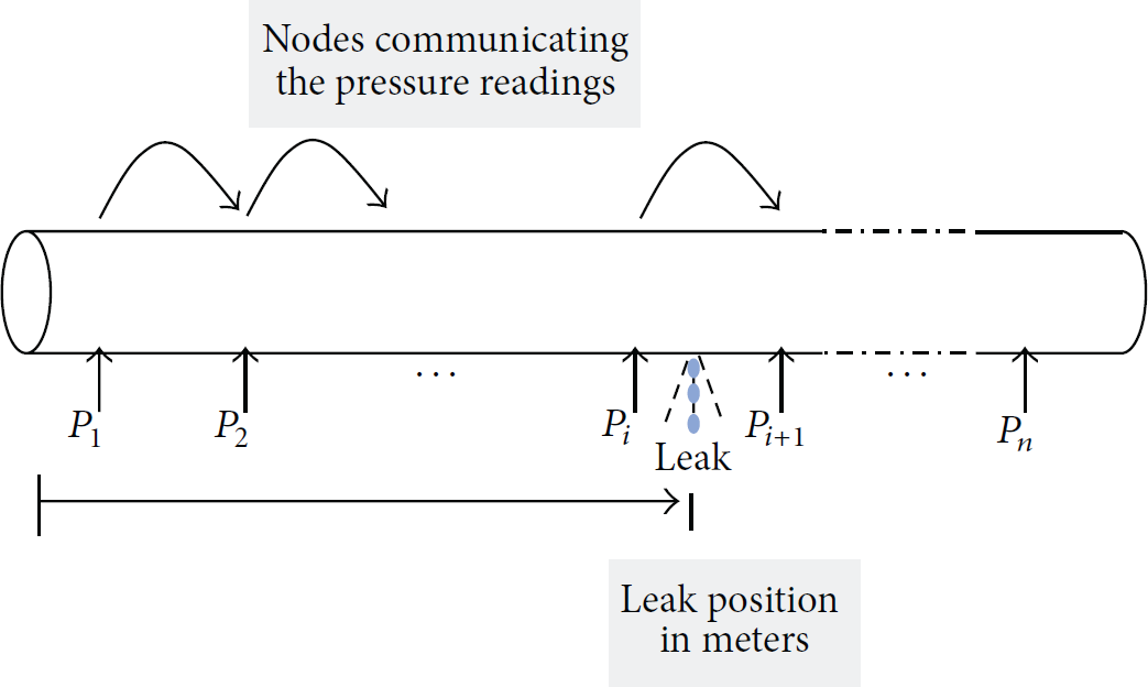
Pipeline setup with uniformly distributed pressure sensor nodes.

Figure 2

Pressure profile across the pipeline.

We also investigate the overall effectiveness of the developed approach from the viewpoint of energy saving. The objective here is achieved by exploiting the DC approach in which the nodes are periodically switched on/off with certain duty cycle in order to save sensing-, communication-, and processing-related energies. Furthermore, the duty cycle increases when a leak is detected, and samples are collected at a faster rate in order to capture the full dynamics of the leak. We also include the DD technique in which the nodes that are closer to the leak point are sampled at a faster rate compared to the ones that are further from the leak point, thus further reducing the energy consumed, but at the cost of some reduction in the accuracy of leak location and size estimation. Ideally (i.e., in a noise-free environment), only two pressure measurements on each side of the leak position are enough to calculate the leak location and size as shown in Figure 2. Therefore, unlike in the first case where all sensors before and after the leak location are used, in the second case, only 4 pressure sensors are used, two on each side of the leak position, and the results of both cases are then compared to each other from both accuracy and energy saving viewpoints.

Under no leak case, all the sensors wake up, collect measurements together with a low sampling rate, and then sleep at the same time but do not communicate any measurement information unless it is above a threshold value which is indicative of leak occurrence and its approximate location. After a leak has been detected, the 4 sensor nodes closest to the candidate leak location then collect pressure measurements at a high sampling rate and communicate this information in order to estimate the leak location and leak growth (i.e., rate of increase of size) using the least-squares estimation technique. The flowchart of the algorithm is given in Figure 3.

Figure 3

Flowchart of the algorithm.

2.1. Simulation Scenario Using EPANET and MATLAB

EPANET software is a program used to simulate water distribution systems. It is used here to simulate a simple pipeline setup and acquire data from it for both analysis and evaluation of our proposed approach. We assume a carbon steel pipe of length 11 km and a diameter of 12 inches. A 1000 KW pump is used, with 11 pressure (labeled as $P_{11}$ , $P_{12}$ , and so on as shown in Figure 4) and 11 flow sensors uniformly distributed along the pipeline.

Figure 4

Snapshot of EPANET simulation environment.

As such EPANET does not have the explicit option to model and simulate the leak, we use instead the sprinkler/nozzle feature in EPANET for this purpose. The emitter coefficient (EC) provides a measure of the size of the leak and is given by the following equation:

$$\begin{array}{cc}& Q=\mathrm{E}\mathrm{C}\times P^{P_{\mathrm{e}\mathrm{x}\mathrm{p}}},\end{array}$$

(1)

where EC is the emitter coefficient, Q is the flow rate, P is the pressure, and $P_{\mathrm{e}\mathrm{x}\mathrm{p}}$ is the pressure exponent and is usually equal to 0.5. The emitter coefficient value varies from 0 to 1. As mentioned before, we assume only single leak occurrence at any one time.

MATLAB is used to access the EPANET model in order make changes in the leak location and size and generate various datasets of pressure and flow rate values (without and with noise) for different leak locations and leak sizes across the pipeline. The MATLAB algorithm is then run using some of the collected pressure and flow data efficiently so as to numerically estimate the leak location and size and calculate the power consumption for the whole process.

2.2. Node's Sensing and Communication Algorithm

The implementation of the proposed strategy will require the following functionality at the node:

• (i)

Nodes will be configured for the threshold value above which the node will report leak detection.

(ii)

A node will operate at a minimum sampling rate in case of no leak. In this mode, the node will keep sampling at a low rate and will not send the sensed value to the sink except for the periodic alive signal with the current value.

(iii)

When the sensed value is above the threshold value, the node will send the former value immediately towards the sink through the local neighborhood cluster.

(iv)

The data sampling at some nodes (where the selection of nodes can be implemented at either the sink or the head of the neighborhood cluster) will be increased to its maximum for better leak sizing and localization.

Since not all the nodes will increase their sampling rate, and the maximum sampling rate should be within the synchronized sampling band of the overall WSN, the following scheme is adhered to:

• (i)

  The sink will collect all the values from the sensor nodes with time stamps for later use.

• (ii)

  The nodes will update the sink with the sensed value only if the error between the currently sensed value and the last transmitted value is more than the allowed error tolerance (e.g., ±1%).

• (iii)

  Nodes will communicate their sensed values to the sink in the following cases:

• (b)

  If currently-sensed_value − last_transmitted_value > error tolerance.

• (c)

  If a potential leak is detected, that is, currently-sensed_value > leak_threshold.

(iv)

The issue of variable sampling requires the MAC level protocol to have the following attributes:

• (a)

The selection of sending nodes can be decided upon by local cooperation (neighborhood cluster fashion) or can be handled by the sink.

(b)

Variable sampling can be a function of the local threshold or can be adjusted by the command from the sink for the selected nodes once a leak has been detected. Recall that, in such circumstances, the increased sampling rate of nodes in the neighborhood of a leak is needed to improve the estimation of both the size and location of the leak.

When a higher sampling rate is called upon, only few nodes will sense and send data at the high rate, while the rest of the nodes in the path towards the sink will work like relaying nodes (i.e., only receiving and transmitting data from other nodes towards the sink).

3. Results and Discussion

As discussed in the previous section, we consider an 11 km pipeline with a node positioned at every 1 km. In the absence of a leak, all the sensor nodes collect measurement with a low sampling rate of 60 seconds as explained in the previous section and as shown in the flowchart in Figure 3. In our EPANET simulation, we introduce a leak at a distance of 7.4 km that grows slowly in one hour from an EC value of 0.01 to 0.91 with an increment of 0.1 at every 10 seconds. The leak present at 7.4 km will be first detected by the node at 8 km which will then trigger the other nearby nodes to increase their sampling rate by collecting data every 1 second instead of every 60 seconds, thus indicating that the nodes will now be continuously sampling (mentioned as high-rate sampling in the flowchart in Figure 3) and communicating their pressure measurements to other nodes to estimate the leak location and size every 1 second using the least-squares technique.

3.1. Estimating the Leak Location and Size Using Both the Full Set and a Reduced (4) Set of Sensors

For leak detection and localization, high-rate sampling is used and we consider measurement uncertainty for the pressure sensors with covariance values 0, 0.00001, 0.0001, and 0.001. Figures 5–7 show the results for estimating the leak position and size with no noise in the sensors measurement. The errors in leak distance and EC, for various leak sizes, are shown in Figures 6 and 7, respectively, with all sensors used as well as with only 4 sensors used. Tables 1 and 2, respectively, show the mean and standard deviation of the error in leak position and size, for leak sizes of 0.01, 0.51, and 0.91. It is clear from the graphs as well as from Tables 1 and 2 that, for small size leaks, the errors in leak position and size are higher, compared to large errors for large leaks. The standard deviation of the error is expectedly zero when no noise is considered in the sensor measurements. As shown in Figure 6, the maximum true percent relative error in leak position is at the smallest leak size, which for no leak is 0.064/11000 × 100 = 5.8182 × 10⁻⁴% and, when using only 4 sensors, is 0.057/11000 × 100 = 5.1818 × 10⁻⁴%.

Table 1

Errors in leak position (in m) considering various uncertainties in measurement noise and number of sensors.

Results for error in leak position
	Noise	Leak size = 0.01		Leak size = 0.51		Leak size = 0.91
		Mean	Std.	Mean	Std.	Mean	Std.
All sensors used	0	−0.056503	0.000000	0.002085	0.000000	0.001623	0.000000
	0.00001	−0.043344	0.128730	0.009666	0.019644	−0.000185	0.009721
	0.0001	−0.283389	1.134237	0.017145	0.085218	−0.008393	0.049021
	0.001	2.353393	13.110680	0.343415	1.017273	0.311415	0.966192
Only 4 sensors used	0	−0.064579	0.000000	0.004041	0.000000	0.002298	0.000000
	0.00001	0.020759	0.239826	−0.000500	0.017903	0.004373	0.013051
	0.0001	0.089133	2.518993	−0.153056	0.283821	−0.006617	0.087127
	0.001	2.432235	19.856501	−0.427856	1.446890	0.295537	0.538968

Table 2

Errors in leak size (EC) considering various uncertainties in measurement noise and number of sensors.

Results for error in leak size
	Noise	Leak size = 0.01		Leak size = 0.51		Leak size = 0.91
		Mean	Std.	Mean	Std.	Mean	Std.
All sensors used	0	0.017556	0.000000	0.000495	0.000000	0.000154	0.000000
	0.00001	0.428051	0.000047	−0.039077	0.000007	−0.411873	0.000004
	0.0001	0.018428	0.006037	0.000346	0.000452	0.000349	0.000260
	0.001	0.013881	0.068662	0.000089	0.005330	−0.006448	0.005019
Only 4 sensors used	0	0.017527	0.000000	0.000460	0.000000	0.000165	0.000000
	0.00001	0.448322	0.000015	−0.046065	0.000001	−0.441423	0.000001
	0.0001	0.017751	0.013386	0.001581	0.001497	−0.000121	0.000462
	0.001	0.016245	0.102970	0.002206	0.007525	−0.011614	0.002818

Figure 5

A final snapshot of simulation is shown in which the leak is at 7400 m (i.e., 7.4 km) from the source, which grows from emitter coefficient value of 0.01 to 0.91 in 1 hour. Pressure measurements at 11 uniformly distributed nodes are shown, and estimated leak position is 7399.9984 and leak size is 0.91015, when all sensors are used.

Figure 6

Assuming no noise in sensor data. Plots of errors in leak position (in m) for various leak sizes with readings from (i) all sensors and (ii) four sensors only.

Figure 7

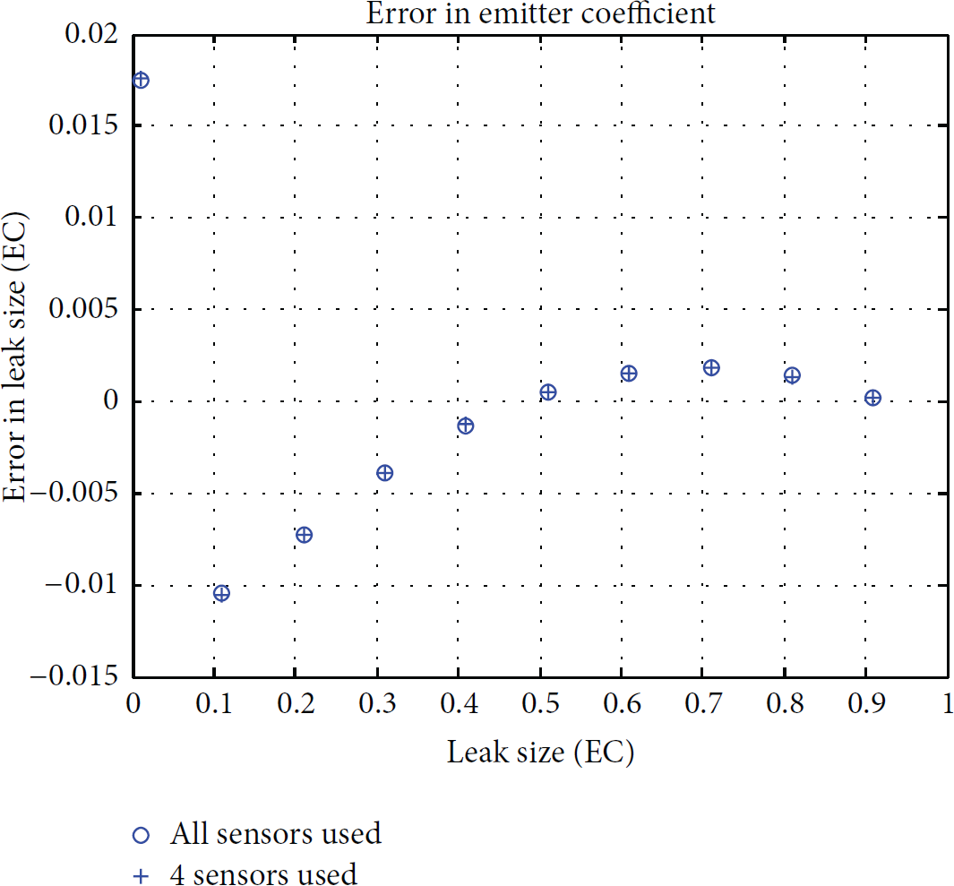
Assuming no noise in sensor data. Plots of errors in leak size (EC) for various leak sizes with readings from (i) all sensors and (ii) four sensors only.

Figure 8 shows the error in leak position (in meters) for various leak sizes, when all the sensors are used and then when only 4 sensors are used with high-rate sampling, when the noise covariance is 0.001. Figure 9 shows similar results for the errors in EC. Tables 1 and 2 show the mean and standard deviation of these errors with high-rate sampling (as shown in the flowchart in Figure 3). For the EC value of 0.01, the standard deviation in the error in leak position is 13.110680 meters when all sensors are used and 19.856501 meters when only 4 sensors are used. This shows that, with this approach and for large measurement noise level such as 0.001, there will be large estimation errors for very small leak sizes. This suggests that, in such cases, the estimation accuracy could be improved if the 4 pressure sensors used are complemented by some other types of sensor (e.g., flow) measurement. But for large leak sizes, such as EC = 0.91, the standard deviations of the errors are 0.966192 m and 0.538968 m and, as such, both are close to each other and acceptable.

Figure 8

Assuming noise covariance of 0.001 in sensor data. Plots of errors in leak position (in meters) for various leak sizes using all sensors (a) and only four sensors (b).

Figure 9

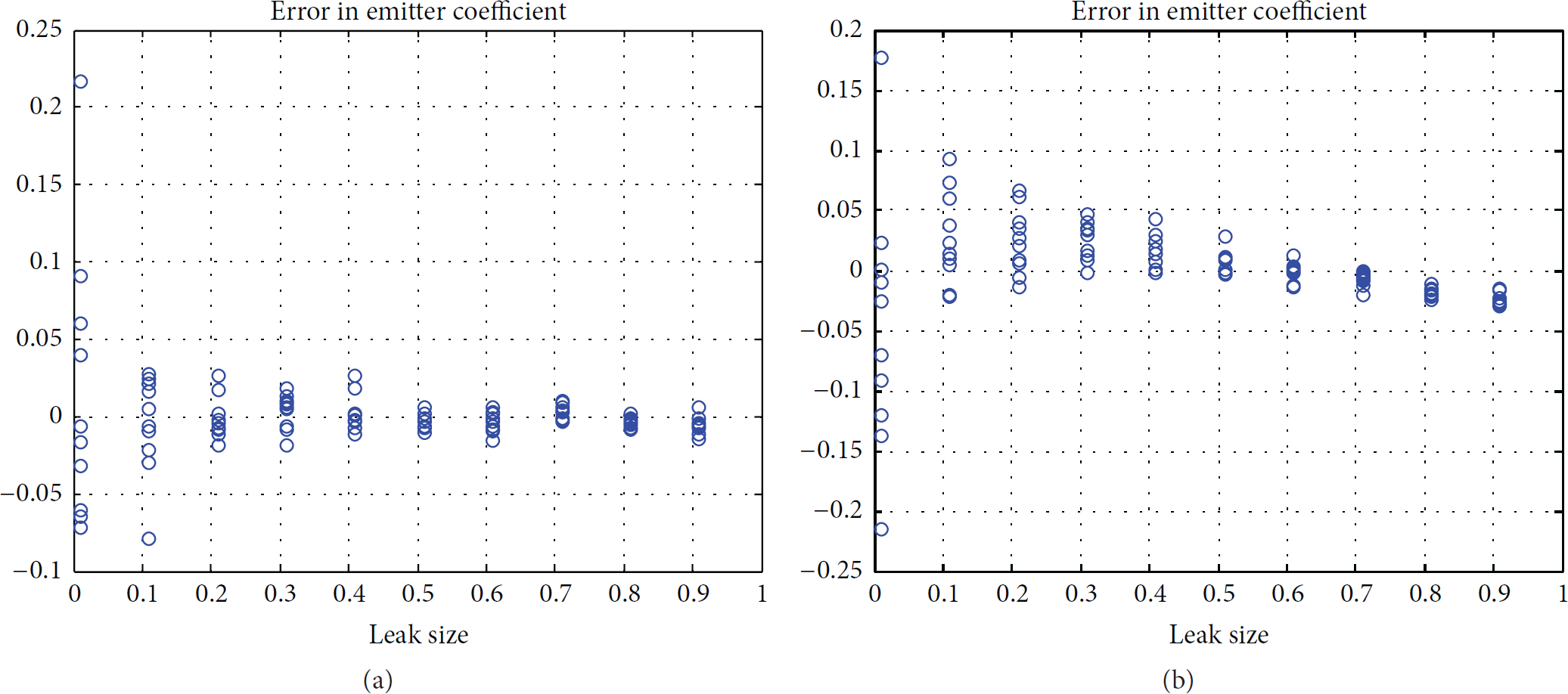
Assuming noise covariance of 0.001 in sensor data. Plots of errors in leak size (EC) for various leak sizes using all sensors (a) and only four sensors (b).

As shown in Figure 8, for noise covariance of 0.001 in sensor data, the maximum true percent relative error in leak position is at the smallest leak size, which for no leak is 37/11000 × 100 = 0.3364% and when using only 4 sensors is 57/11000 × 100 = 0.5182%. This means a small increase in error by $(57-37)/11000\times 100=0.1818$ %. Increase in error in emitter coefficient is up to $(0.22-0.178)/0.22\times 100=19.1$ %. Error of EC = 0.22 − 0.178 = 0.042 is equivalent to an error of 0.4444 litres/sec, as per (1).

3.2. Energy Calculation and Saving

Here, each pressure sensor node consumes power in all of its 3 elements, that is, the sensor, microcontroller, and radio communication. Table 3 shows the components whose specifications are used to calculate the energy consumption during monitoring under “no leak” and “leak” conditions.

Table 3

Power consumption specifications for the 3 elements in a sensor node.

Type of component	Device name	Power consumption specifications
Pressure sensor	Honeywell ASDX silicon series pressure sensors [20]	5 V × 2.5 mA = 12.5 mW
Microcontroller	8-bit Atmel with programmable flash [21]	Power down mode: 1.8 V × 0.1 µA = 0.18 µW
		Active mode: 1.8 V × 500 µA = 900 µW
Radio communication module	Mica2 [22]	Transmission power = 60 mW
		Receiving power = 45 mW

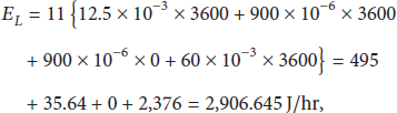
Energy consumed when a leak occurs is   

$$\begin{array}{cc}& E_L=E_s+E_{\mu ca}+E_{\mu ci}+E_{rd},\end{array}$$

(2)

where    $E_s$ is the energy consumed by the sensor, $E_{\mu ca}$ is the energy consumed by the microcontroller in active mode, $E_{\mu ci}$ is the energy consumed by the microcontroller in idle mode, and $E_{rd}$ is the energy consumed in communication (includes the time to create connection, transmitting, and receiving, in single hop)

Energy consumed when no leak occurs is

$$\begin{array}{cc}& E_{\mathrm{N}\mathrm{L}}=E_{\mathrm{N}{\mathrm{L}}_s}+E_{\mathrm{N}{\mathrm{L}}_{\mu ca}}+E_{\mathrm{N}{\mathrm{L}}_{\mu ci}}+E_{\mathrm{N}{\mathrm{L}}_{rd}},\\ E_{\mathrm{N}\mathrm{L}}=n\left(P_s{T}_{{\mathrm{N}\mathrm{L}}_s}+P_{\mu ca}{T}_{\mathrm{N}{\mathrm{L}}_{\mu ca}}+P_{\mu ci}{T}_{\mathrm{N}{\mathrm{L}}_{\mu ci}}+P_{rd}{T}_{\mathrm{N}{\mathrm{L}}_{rd}}\right),\end{array}$$

(3)

where $P_s$ denotes power consumption of sensor = 12.5 mW (Table 2), $P_{\mu ca}$ denotes power consumption of microcontroller in active mode = 900 μW, $P_{\mu ci}$ denotes power consumption of microcontroller in idle mode = 0.18 μW, and $P_{rd}$ denotes power consumption by the radio = 45 or 60 mW. A typical value of 60 W is considered because all the nodes (except the end nodes) transmit and receive. n is the number of sensor nodes (a sensor node is a complete unit including sensor element, transducer, microcontroller, and transceiver) and $T_{{\mathrm{N}\mathrm{L}}_s}$ is the time needed by the sensor to collect a sample; a duty cycle of 1/60 is considered here. $T_{\mathrm{N}{\mathrm{L}}_{\mu ca}}$ is the time for which the microcontroller is in active mode for processing sensor measurement and communicating; a duty cycle of 1/60 is considered here. $T_{\mathrm{N}{\mathrm{L}}_{\mu ci}}$ is the time for which the microcontroller is in idle mode and not processing sensor measurement and communicating; a duty cycle of 59/60 is considered here. $T_{\mathrm{N}{\mathrm{L}}_{rd}}$ is the time for which radio is on, transmitting and receiving; this is zero in case of no leak, as there is no communication between the nodes.

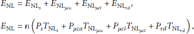
Energy consumed in monitoring for 1 hour by the given 11 nodes is

$$\begin{array}{cc}& E_{\mathrm{N}\mathrm{L}}=\mathrm{11}\left\{\mathrm{12.5}\times {\mathrm{10}}^{-\mathrm{3}}\times \mathrm{60}+\mathrm{900}\times {\mathrm{10}}^{-\mathrm{6}}\times \mathrm{60}+\mathrm{900}\times {\mathrm{10}}^{-\mathrm{6}}\times \left(\mathrm{3600}-\mathrm{60}\right)+\mathrm{60}\times {\mathrm{10}}^{-\mathrm{3}}\times \mathrm{0}\right\}=\mathrm{8.25}+\mathrm{0.594}+\mathrm{7.0092}\times {\mathrm{10}}^{-\mathrm{3}}+\mathrm{0}=\mathrm{8.851}\hspace{0.17em}\mathrm{J}/\mathrm{h}\mathrm{r}.\end{array}$$

(4)

In case of a leak, the data sampling will be faster, that is, 1 sample/sec (instead of 1 sample per 60 seconds, as was in the “no leak” case). Therefore, $T_{Ls}$ , $T_{L_{\mu ca}}$ and $T_{L_{rd}}$ will all have a duty cycle of 60/60, and $T_{L_{\mu ci}}$ will have a duty cycle of 0/60; that is, the microcontroller will not go into idle state at all.

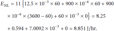
Therefore, the energy consumed in monitoring the given leak for 1 hour is given by

$$\begin{array}{cc}& E_L=\mathrm{11}\left\{\mathrm{12.5}\times {\mathrm{10}}^{-\mathrm{3}}\times \mathrm{3600}+\mathrm{900}\times {\mathrm{10}}^{-\mathrm{6}}\times \mathrm{3600}+\mathrm{900}\times {\mathrm{10}}^{-\mathrm{6}}\times \mathrm{0}+\mathrm{60}\times {\mathrm{10}}^{-\mathrm{3}}\times \mathrm{3600}\right\}=\mathrm{495}+\mathrm{35.64}+\mathrm{0}+\mathrm{2}\text{,}\mathrm{376}=\mathrm{2}\text{,}\mathrm{906.645}\hspace{0.17em}\mathrm{J}/\mathrm{h}\mathrm{r},\end{array}$$

(5)

which represents a huge hike of 328 times more energy consumption when compared to monitoring in the “no leak” case.

We presented results in the previous section that show that, even in the presence of noise, simply using data from 4 sensor nodes can give results of acceptable accuracy except for the case of small size leaks. The energy consumed in using 4 sensors only will be the sum of energies consumed by the 4 sensors operating at high-rate sampling with the remaining 7 operating at low-rate sampling, that is, = $E_L$ (with 4 active sensors) = $(\mathrm{2,906.645}/11)\times 4+(8.851/11)\times 7=$ 1,118.919 J/hr.

This clearly shows an appreciable and active reduction in energy consumption by 2.6 times by using only 4 sensor nodes, that is, with a 2.75 times' decrease $\left(11/4=2.75\right)$ in the number of active sensors. By way of assessing the impact of our proposed energy reduction scheme on the estimation accuracy of both leak size and location, we estimate that a $61.5\%$ (= ((2,906.645 − 1,118.919)/2,906.645) × 100%) overall reduction in power results in an increase in error by up to (57 − 37)/11000 × 100 = 0.1818% in the leak location and an increase in error of up to (0.22 − 0.178)/0.22 × 100 = 19.1% in the emitter coefficient, as shown in the results of Figures 8 and 9 for the smallest leak size of emitter coefficient value of 0.01 and the highest sensor noise covariance of 0.001. These results are comparable to the results acquired in [15] in a DC-DD-based fusion approach for weather monitoring, where the estimation error increased by 16.1% by reducing the energy consumption to 70% in an outdoor experiment using the measurements of temperature, pressure, wind velocity, and humidity. In another experiment of theirs (in [15]), which was performed in an indoor environment using the measurements of temperature and humidity, the error increased by 36.2% by reducing the energy consumption to 60%.

4. Conclusion and Future Work

We conclude that, with less sensor measurement noise, using only 4 sensors to estimate the leak location and size gives results of significant accuracy (i.e., error in leak position is less than 1 meter even for very small leak sizes). Note here that results achieved by using data from all sensor nodes are more accurate, but at the cost of higher energy consumption. An attractive reduction by a factor of 2.6 was achieved in the energy consumed by sensing, communication, and processing tasks when only 4 sensors are sampled at a higher rate for leak localization, while other sensors are sampled at a normal rate for capturing any other events or detecting leaks in the rest of the pipeline.

The attractive results achieved in this study based on single leak detection give ample encouragement to extend it to more complex pipeline structures, using various types of sensors (such as flow measurement, vibration, and hydrophones). Such an extension will also allow us to investigate some tradeoffs between accuracy and reliability on the one hand and energy minimization on the other hand, in our selection of sensors since some of these are more accurate but also more energy hungry, while others are less accurate and less reliable but consume only small energy. Future work also includes the development of a dynamic reconfiguration-based MAC protocol for the required heterogeneous communication among the sensors and the sink node. Finally, as a way to further reduce the energy consumption, our efforts to use energy harvesting are currently underway.