Multivariate Statistical Approach for Anomaly Detection and Lost Data Recovery in Wireless Sensor Networks

Abstract

Data loss due to integrity attacks or malfunction constitutes a principal concern in wireless sensor networks (WSNs). The present paper introduces a novel data loss/modification detection and recovery scheme in this context. Both elements, detection and data recovery, rely on a multivariate statistical analysis approach that exploits spatial density, a common feature in network environments such as WSNs. To evaluate the proposal, we consider WSN scenarios based on temperature sensors, both simulated and real. Furthermore, we consider three different routing algorithms, showing the strong interplay among (a) the routing strategy, (b) the negative effect of data loss on the network performance, and (c) the data recovering capability of the approach. We also introduce a novel data arrangement method to exploit the spatial correlation among the sensors in a more efficient manner. In this data arrangement, we only consider the nearest nodes to a given affected sensor, improving the data recovery performance up to 99%. According to the results, the proposed mechanisms based on multivariate techniques improve the robustness of WSNs against data loss.

1. Introduction

A wireless sensor network (WSN) is a (structured or not) group of hundreds or even thousands of sensor devices intended to monitor a given area or region by measuring one or more physical variables [1]. Typically, a central unit (CU) exists to gather and analyze the data generated by the sensors. The data collected by the sensors can be transmitted to the CU either directly or through the collaboration of several of the devices in the network using multihop routing. It may also be useful to arrange the sensors in groups (clusters) for data aggregation, so that the manager node in the cluster is responsible for collecting and sending the data to the CU. Data aggregation reduces the energy consumption, which is an attractive goal for this kind of networks.

There are two principal WSN uses: monitoring and tracking. In both cases, WSNs can be applied in various fields, including the military, medical, and/or industrial fields [2]. These networks are usually assumed to contain fixed nodes. However, providing nodes with mobility has several advantages in terms of connectivity, cost, reliability, and energetic efficiency [3].

Deploying monitoring mechanisms in WSNs to strengthen the services provided is encouraged. This is especially true in hostile environments like military actions, crisis management, and disaster detection and recovery, where data loss or data modification can lead to disastrous consequences. These monitoring mechanisms are especially challenged by malicious data modification attacks, such as the so-called data tampering, environmental tampering, or tampering attack [4, 5].

In the present work, we assess the application of multivariate analysis techniques for WSN monitoring and data recovery. Multivariate techniques fit well when there exists a high temporal and spatial correlation between the variables considered, which is a common feature in WSNs. The monitoring scheme is aimed at finding anomalous records. Subsequently, the diagnosis of these anomalies can show whether the anomaly is due to an actual reading or due to data loss/modification. In the event of data loss/modification, the recovery scheme is responsible for the estimation of the missed data. To monitor and detect anomalies in the system behavior, multivariate statistical process control (MSPC) based on principal component analysis (PCA) [6, 7] and partial least squares (PLS) [8, 9] is used. To recover lost data, trimmed scores regression (TSR) [10, 11] using both PCA- and PLS-based models (TSR-PCA and TSR-PLS) is employed. To the best of our knowledge, this is the first time that MSPC, PLS, and TSR are used in the context of WSNs.

A relevant issue when applying multivariate techniques is the data arrangement, that is, the way collected data are organized to make the most of a multivariate model. This matter has been widely studied in fields like statistical monitoring, process control, or image processing and has a significant impact depending on the application at hand. We evaluate the impact of data arrangement on the recovery of lost data and show that the recovery performance can be improved by merely rearranging the data in a certain way.

Finally, we show that the routing algorithm chosen for multihop retransmissions has a relevant influence on the data loss/modification impact on network performance. We analyze three routing scenarios to evidence the consequences on the number of sensors affected depending on both the routing algorithm used and the location of the specific sensor under tampering attack or malfunction. Afterwards, we test the performance of our system and show how to detect and recover the original values of the affected sensors through the previously mentioned multivariate techniques.

In summary, we make three main contributions in this work:

• (i)

The assessment of a multivariate statistical-based response scheme to detect data loss/modification and recover missing data.

(ii)

The deployment of a neighborhood-based data imputation scheme through a local data arrangement to take advantage of the higher correlation between closer sensors.

(iii)

The analysis of how the underlying multihop routing algorithm modifies the consequences of the data tampering attack.

The rest of the paper is organized as follows. Section 2 presents some relevant works related to the subject under study. Section 3 discusses the fundamentals of the multivariate analysis techniques used in the present work, and Section 4 introduces their use in missing data recovery. Section 5 describes two different methods to arrange the original data for modeling and the importance of this choice depending on the system purposes. Section 6 presents a simulation scenario and the associated recovery performance results. Section 7 illustrates a procedure to improve the results obtained using local models in order to exploit the high correlation between close sensors. In Section 8, a real WSN scenario is considered to corroborate the validity of the results when the proposal is executed over a real environment. Finally, Section 9 discusses the principal conclusions and remarks on this work as well as some future research directions.

2. Related Work

Several anomaly detection and missing data imputation techniques for WSNs have been recently proposed. A neural network-based anomaly detection scheme and a missing data imputation algorithm were developed in [12]. The network is partitioned into clusters, and the missing data algorithm selects the nearest neighbor or the most repeated value of the neighbors to estimate the missing value for the target sensor. If there are no neighbors, the last value of the sensor is chosen instead. In this case, the missing data imputation technique is used to improve the performance of the classification process by the neural network. Aiming at obtaining reliable health monitoring systems, the work addressed in [13] proposes a distributed scheme to detect and isolate those sensors whose measurements are missing or are inaccurate. This is carried out by using analytical redundancy taking into account the inherent redundant information in these systems. This way, a virtual predicted value per each observed sensor value is computed. The virtual values are nonfaulty and will be obtained from the measured outputs of correlated sensors and the previously acquired system knowledge. Thus an inconsistency value will be detected through the residuals obtained when comparing both, virtual and observed values. The authors in [14] introduce a data mining methodology based on exploiting spatial-temporal relationships among sensors in WSNs for missing data imputation. Another study [15] addresses a robust method to recover missing data using two temporal predictors and one spatial predictor. The algorithm selects the best predictor among the three when there are missing data, showing how sampling rate and packet loss affect recovery accuracy. A missing data recovery proposal using sparsity-spatial interpolation with a fixed Discrete Cosine Transform (DCT) basis is addressed in [16]. Another study further proposes a sparsity-based missing data recovery method [17] to enhance the previous work. Reference [18] develops a novel anomaly detection and missing data imputation technique using dynamic Bayesian networks to exploit spatial and temporal correlation among samples. If there is a discrepancy between the normality model (data calibration-based model) and the actual sensor value, an anomaly alarm is triggered. The imputation or recovery method is then addressed by inferring the most likely sensor value from both the current and immediate past values. As in the previous work, the authors in [19] consider the inherent spatial and temporal correlation commonly exhibited in this type of networks. The work proposes a nearest neighbor (NN) missing data imputation scheme through the use of $k\text{-}d$ trees. They are built by considering weighted variances and weighted Euclidean distances obtained from measured percentages of missing data. Their missing data NN algorithm will use the nearest neighbors found in $k\text{-}d$ tree traversal to impute the lost sensor value. Reference [20] addresses the distributed $H_{\infty }$ filtering problem in sensor networks in presence of missing data. Each sensor is provided by a specific filter, designed to maintain a constant prediction error and to accomplish a predefined performance according to their own and adjacent values.

Although multivariate methodologies have been extensively used in the literature, their application to WSNs is limited. Until now, few works make use of multivariate analysis in WSNs, and most of them are limited to intrusion or anomaly detection, not data recovery. An intrusion detection system for routing attacks based on PCA is introduced in [21]. The authors partition the network into groups with one monitor per group. Each monitor has two PCA models: one for its own traffic and one for the global traffic, which is obtained by exchanging its local PCA model with other monitors. The authors conclude that a PCA global distributed modeling achieves better detection performance than the centralized modeling for sinkhole attacks (sinkhole attacks are those in which a malicious node sends fake routing information claiming an optimum route to make other nodes route data packets through the malicious node to inspect and filter the traffic). A PCA-based anomaly detection is proposed in [22]. In that reference, the authors develop a system with two phases: data modeling and anomaly detection. For data modeling, two methods are discussed to improve PCA modeling against outliers or inconsistent data. The anomaly detection process is then performed by comparing calibration data with new incoming data using the Mahalanobis distance.

Given the general high performance exhibited by multivariate techniques in several heterogeneous fields, we assess in this paper a multivariate scheme for anomaly detection, data loss identification, and missing data recovery using latent variable models. When latent variable techniques are employed, main design choices are the data arrangement and the selection of the number of latent variables. The problem of optimum data arrangement for multivariate modeling is treated in a considerable number of references, covering applications such as statistical monitoring [23], process control [24], or image processing [25]. For instance, Dynamic PCA [26], which has raised a great interest in the scientific community, is simply a data rearrangement process followed by a traditional PCA modeling. Previous references show that the data arrangement problem is a paramount topic to incorporate dynamics, locality, and/or segmentation in a multivariate model. It is also accepted that the optimum arrangement is application dependent [27], so that it needs to be carefully chosen for each particular application. This paper addresses the data arrangement for both anomaly detection and data recovery.

3. Multivariate Statistical Analysis

Most natural and man-made processes are multivariate systems, as their adequate characterization requires the joint use of several variables. For instance, weather forecasting depends on wind, atmosphere pressure, and temperature, among many other factors.

Data description and modeling, discrimination and classification, or regression and prediction [28] are the usual fields for applying multivariate techniques. The following sections provide the fundamentals of multivariate statistical analysis in the context of this work.

3.1. PCA: Principal Components Analysis

The main goal of PCA is data compression. PCA identifies a number of linear combinations of the original variables in a data set X, the so-called principal components (PCs), containing most of its relevant information (variability). This is a change of variables from the original variables in the X space to the PCs subspace. If X is a data matrix with J variables associated with a given phenomenon and I observations of each variable, PCA reduces its dimension from J variables to A PCs by finding the A-dimensional latent subspace of most captured variability.

PCA follows the next equation:

$$\begin{array}{cc}& \mathbf{X}={\mathbf{T}}_A·{\mathbf{P}}_A^T+{\mathbf{E}}_A,\end{array}$$

(1)

where ${\mathbf{P}}_A$ is the $J\times A$ loading matrix, ${\mathbf{T}}_A$ is the $I\times A$ score matrix, and ${\mathbf{E}}_A$ is the $I\times J$ residual matrix. The maximum variance directions are obtained from the eigenvectors of ${\mathbf{X}}^T·\mathbf{X}$ , and they are ordered as the columns of ${\mathbf{P}}_A$ by explained variance. The rows of ${\mathbf{T}}_A$ are the projections of the original I observations in the new latent subspace. ${\mathbf{E}}_A$ is the matrix that contains the residual error, and it plays a crucial role in anomaly detection, as shown afterwards. The projection (score) on the PCA subspace of a new observation is obtained as follows:

$$\begin{array}{cc}& {\mathbf{t}}_{\text{new}}={\mathbf{x}}_{\text{new}}·{\mathbf{P}}_A,\end{array}$$

(2)

where ${\mathbf{x}}_{\text{new}}$ is a $\mathrm{1}\times J$ vector representing a new object and ${\mathbf{t}}_{\text{new}}$ is a $\mathrm{1}\times A$ vector representing its projection to the latent subspace.

The number of PCs in a model, A, can be selected using several methods, including cross-validation [29, 30]. Section 3.3 introduces this method.

3.2. PLS: Partial Least Squares

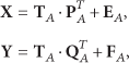
Another relevant problem in multivariate analysis is data regression, where two data sets are involved, X and Y, where X is the $I\times J$ measurement matrix used to predict Y ( $I\times M$ ).

To predict Y, a model B containing the regression relationship between both data sets X and Y is first estimated. New Y values can then be predicted from the new X measures. The linear regression problem is defined by the expression

$$\begin{array}{cc}& \mathbf{Y}=\mathbf{X}·\mathbf{B}+\mathbf{F}\mathbf{.}\end{array}$$

(3)

The least squares solution for (3) is

$$\begin{array}{cc}& \widehat{\mathbf{B}}={\left({\mathbf{X}}^T·\mathbf{X}\right)}^{-\mathrm{1}}·{\mathbf{X}}^T·\mathbf{Y}\mathbf{.}\end{array}$$

(4)

This solution cannot be computed if matrix ${\mathbf{X}}^T·\mathbf{X}$ is singular. It is also highly unstable when a high correlation exists among variables in X. To overcome this limitation, the PLS method applies the latent PCA subspace idea to the regression problem. In this case, the variables in X are transformed to a reduced set of latent variables that maximize the covariance between X and Y.

The partial linear regression problem between normalized matrices X and Y can be stated as

$$\begin{array}{cc}& \mathbf{X}={\mathbf{T}}_A·{\mathbf{P}}_A^T+{\mathbf{E}}_A,\\ \mathbf{Y}={\mathbf{T}}_A·{\mathbf{Q}}_A^T+{\mathbf{F}}_A,\end{array}$$

(5)

where ${\mathbf{T}}_A$ is the $I\times A$ score matrix, ${\mathbf{P}}_A$ and ${\mathbf{Q}}_A$ are the $J\times A$ and $M\times A$ loading matrices, and ${\mathbf{E}}_A$ and ${\mathbf{F}}_A$ are the $I\times J$ and $I\times M$ residual matrices of X and Y, respectively.

The regression coefficients of the PLS model are finally established as

$$\begin{array}{cc}& {\widehat{\mathbf{B}}}_{\text{PLS}}=\mathbf{W}·{\left({\mathbf{P}}^T·\mathbf{W}\right)}^{-\mathrm{1}}·{\mathbf{Q}}^T,\end{array}$$

(6)

where W is a $J\times A$ matrix of weights, such that $\mathbf{T}=\mathbf{X}·\mathbf{W}·{\left({\mathbf{P}}^T·\mathbf{W}\right)}^{-\mathrm{1}}$ . A PLS model is thus represented by matrices P, W, and Q.

Finally, a new observation with the PLS model is estimated as

$$\begin{array}{cc}& {\widehat{\mathbf{y}}}_{\text{new}}={\mathbf{x}}_{\text{new}}·{\widehat{\mathbf{B}}}_{\text{PLS}},\end{array}$$

(7)

where ${\mathbf{x}}_{\text{new}}$ is a $\mathrm{1}\times J$ vector representing a new object and ${\widehat{\mathbf{y}}}_{\text{new}}$ is a $\mathrm{1}\times M$ vector representing the estimation of the output variables.

The number of dimensions of the latent subspace, A, can be also estimated through cross-validation.

3.3. Selection of the Number of Latent Variables: Cross-Validation

The prediction ability of a model is related to its capacity to estimate new data previously unseen during the calibration (or training) phase. The usual way to assess the prediction performance of a model is using a validation set [28]. In a validation set, different data than those used in the calibration process are considered. The so-called cross-validation procedure is a good validation option when the number of observations in a given data set is small.

The central idea in cross-validation is to divide the available observations into G groups and compute the prediction errors for each of them. In each iteration, the calibration model is obtained from $G-\mathrm{1}$ groups, while the remaining group is predicted from the model and the corresponding prediction error is computed. This process is repeated for all groups, and the total error is obtained for the resulting G combinations.

Wold [29] proposed the use of cross-validation to determine the number of PCs in PCA. The prediction error (typically Prediction Error Sum of Squares, or PRESS) obtained in the cross-validation process is computed when the number of PCs equals one, two, and so on. Finally, the number of PCs is selected from the PRESS shape.

Cross-validation can be directly applied to PLS models. However, this is not possible for PCA models because the notion of prediction error in PCA is ill defined. This is because PCA models are not prediction models, and a prediction procedure can not be univocally stated. The authors in [31] conclude that the element-wise k-fold (ekf) algorithm is a valid choice for PCA cross-validation when the model is used for missing data imputation purposes, as in the present paper. See the Appendix for a brief explanation of the ekf algorithm.

3.4. Multivariate Statistical Process Control

One of the most extended applications of PCA and PLS is process monitoring and anomaly detection and diagnosis, often referred to as multivariate statistical process control (MSPC). In a MSPC system, Q and $T^{\mathrm{2}}$ [32] statistics are commonly used. Q compresses the residuals in each observation, and $T^{\mathrm{2}}$ is computed from the scores. With both statistics computed from the calibration data under normal conditions, control limits can be established with a certain confidence level. New data are then monitored using these limits. An anomaly is identified when the limits are exceeded. Furthermore, the contribution of the variables to a detected anomaly can be investigated with the contribution plots [33].

The Q and $T^{\mathrm{2}}$ statistics for a specific observation can be computed using the following equations:

$$\begin{array}{cc}& T_i^{\mathrm{2}}={\displaystyle \sum }_{a=\mathrm{1}}^A{\left(\frac{{\tau }_{ai}-{\mu }_a}{{\sigma }_a}\right)}^{\mathrm{2}},\end{array}$$

(8)

$$\begin{array}{cc}& Q_i={\displaystyle \sum }_{j=\mathrm{1}}^J{\left(e_{ij}\right)}^{\mathrm{2}},\end{array}$$

(9)

where ${\tau }_{ai}$ represents the score of the ith observation of the ath latent variable, ${\mu }_a$ and ${\sigma }_a$ stand for the mean and standard deviation for the scores of that variable in the calibration data, respectively, and $e_{ij}$ represents the residual value corresponding to the ith observation of the jth variable.

Note that the optimum number of latent variables in the prediction sense does not necessarily match the optimum number for process monitoring [30].

3.5. Suitability Multivariate Techniques in WSNs

A WSN is composed of a set of strategically distributed sensors for gathering some kind of sensed data at a specific sampling rate. Data are then processed for heterogeneous purposes like monitoring or tracking. This way, the information gathered from a WSN could be seen as a set of J variables, the sensors, and a set of I observations, the sensed data at each sampling time. This information has a suitable form to be analyzed with multivariate methods. Besides, multivariate techniques work well with correlated data, a common characteristic in WSN. To briefly justify the use of multivariate techniques in WSNs, we will use a real WSN data set obtained from the LUCE (Lausanne Urban Canopy Experiment) (LUCE deployment data set at http://lcav.epfl.ch/page-86035-en.html) project. More detailed explanation about LUCE deployment and the devised experiments will be detailed in Section 8. Figure 1 illustrates the LUCE data set arrangement to conform the X calibration set considering 61 sensors and 431 time observations of each.

Figure 1

X data set arrangement, conformed by $I=\mathrm{431}$ observations of $J=\mathrm{61}$ variables each from the LUCE experiment deployment.

As mentioned above, the information gathered from a WSN is highly correlated and, therefore, is adequate to be analyzed with multivariate methods. To verify that statement, the intervariable correlation was computed in the LUCE data set, and a minimum correlation coefficient of 0.89 was found. In Figure 2, the residual variance obtained from the PCA model of the real data set in terms of the number of PCs is shown. As a consequence of the high correlation among variables, PCA is able to capture almost all data variability by using only one PC: 97% of the explained variance is obtained while the residual variance is around 3%. In summary, this simple experiment illustrates the suitability of multivariate techniques in WSNs.

Figure 2

Residual variance obtained through the PCA modeling in the LUCE experiment as the number of PCs is increased.

4. Missing Data Recovery

There are several methods and proposals to estimate missing data with PCA. These methods can be classified into two groups: regression and non-regression-based methods, the former ones exhibiting better performance [10]. Among the regression-based techniques, the trimmed scores regression presents a good trade-off between simplicity and estimation performance [11].

The trimmed scores regression (TSR) method estimates the value of the scores from the trimmed scores, that is, the scores obtained by filling the missing values with zeros. For data centered before PCA, this is equivalent to using the average value of a variable to give an initial estimation of its missing values.

Without loss of generality, let us assume an incomplete observation $x_{\text{inc}}$ with available measurements on the first k variables and where the values of the remaining variables are missing. The trimmed scores of $x_{\text{inc}}$ are calculated in PCA as follows:

$$\begin{array}{cc}& {\tau }_A^{\ast }={\left({\mathbf{P}}_{A,k}^{\ast }\right)}^T·x_{\text{inc}}^{\ast },\end{array}$$

(10)

where

$$\begin{array}{cc}& {\mathbf{P}}_{A,k}^{\ast }=\left[\begin{array}{ccc}{p}_{\mathrm{1,1}}& \cdots & p_{A,\mathrm{1}}\\ ⋮& \ddots & ⋮\\ p_{\mathrm{1},k}& \cdots & p_{A,k}\end{array}\right],\\ x_{\text{inc}}^{\ast }={\left[x_{\mathrm{1}},\dots ,x_k\right]}^T,\end{array}$$

(11)

where $p_{a,j}$ is the loading corresponding to the jth variable in the ath PC. Only the available variables in $x_{\text{inc}}$ and their corresponding loadings are thus used to compute the trimmed scores.

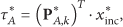
The calibration data in X can be used to improve the estimation of the scores from incomplete observations. Let us call ${\mathbf{X}}^{\ast }$ the submatrix of X with the available variables in $x_{\text{inc}}$ . The matrix of trimmed scores corresponding to the calibration data can be computed as follows:

$$\begin{array}{cc}& {\mathbf{T}}_A^{\ast }={\mathbf{X}}^{\ast }·{\mathbf{P}}_A^{\ast }.\end{array}$$

(12)

The complete score matrix ${\mathbf{T}}_A$ can be regressed on the trimmed scores ${\mathbf{T}}_A^{\ast }$ , such that

$$\begin{array}{cc}& {\mathbf{T}}_A={\mathbf{T}}_A^{\ast }·\mathbf{B}+\mathbf{F}\mathbf{,}\end{array}$$

(13)

where the matrix of regression coefficients B may be computed from least squares, as the inversion of ${\left({\mathbf{T}}_A^{\ast }\right)}^T·{\mathbf{T}}_A^{\ast }$ is typically nicely conditioned. If it is not, PLS or other biased methods can be used to estimate B. Afterward, B is used to improve the score estimation as follows:

$$\begin{array}{cc}& {\tau }_A^{\text{TSR}}={\left({\mathbf{P}}_A^{\ast }·\mathbf{B}\right)}^T·x_{\text{inc}}^{\ast }.\end{array}$$

(14)

Finally, the score ${\tau }_A^{\text{TSR}}$ can be used to estimate the incomplete observation, including its missing elements:

$$\begin{array}{cc}& \widehat{x}={\mathbf{P}}_A·{\tau }_A^{\text{TSR}}.\end{array}$$

(15)

TSR is more efficient as the intervariable correlation in the original data set increases, since variables with missing data for a given observation are computed from available values in others.

In PLS, the trimmed scores of $x_{\text{inc}}$ in (10) are calculated as follows [27]:

$$\begin{array}{cc}& {\tau }_A^{\ast }={\left({\mathbf{R}}_A^{\ast }\right)}^T·x_{\text{inc}}^{\ast },\end{array}$$

(16)

where

$$\begin{array}{cc}& {\mathbf{R}}_A^{\ast }=\left({\mathbf{W}}_{A,k}^{\ast }\right)·{\left({\mathbf{P}}_A^T·{\mathbf{W}}_A\right)}^{-\mathrm{1}}.\end{array}$$

(17)

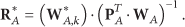
Recall that ${\mathbf{W}}_A$ is the weight matrix and ${\mathbf{P}}_A$ the loading matrix of the PLS model with A latent variables. Conversely, ${\mathbf{W}}_{A,k}^{\ast }$ is expressed as

$$\begin{array}{cc}& {\mathbf{W}}_{A,k}^{\ast }=\left[\begin{array}{ccc}{w}_{\mathrm{1,1}}& \cdots & w_{A,\mathrm{1}}\\ ⋮& \ddots & ⋮\\ w_{\mathrm{1},k}& \cdots & w_{A,k}\end{array}\right],\end{array}$$

(18)

where $w_{a,j}$ is the weight corresponding to the jth variable in the ath latent variable. The complete matrices ${\mathbf{P}}_A$ and ${\mathbf{W}}_A$ are used in the inversion in (17). The information of the complete model is used, improving prediction capability. Moreover, inversion problems are avoided.

For the sake of clarification, a graphical illustration of the missing data recovery method proposed is shown in Figure 3. Note that this procedure is based on the use of PCA models, though considering PLS models does not change the main methodology.

Figure 3

Illustration of the main steps implied in the missing data recovery procedure.

The recovery procedure is activated when an altered observation is detected. A missing data is determined through a previously established monitoring system (that procedure will be detailed in Section 6.2). Although the process is self-explanatory ( $T3$ and $T5$ values are missed and thus they are recovered and substituted by $R3$ and $R5$ , resp.), two are the main aspects to remark here: (i) the imputation method only considers the available information to estimate the scores and (ii) the system is able to get an estimation of the original observation by applying the complete calibration PCA model.

5. Data Arrangement for System Modeling

It should be noted that the data arrangement procedure has a significant impact on the performance of a multivariate model. Furthermore, the suitability of one or another arrangement depends on the purpose of the modeling process itself [34].

As already mentioned and it will be evidenced in Sections 6 and 7, the proposed multivariate approach is applied to both detect anomalies and identify and recover data loss. A different data arrangement to generate the multivariate model is proposed for the monitoring and recovery systems, as the particular conditions and requirements differ. The rest of the section discusses a global model to be used for detection purposes and a local model for data recovery. Though the application of the global model for data recovery is also discussed, the local models are shown to yield a better performance.

5.1. Monitoring: Global Modeling

We define a global model as a PCA model calibrated from the data gathered by the WSN arranged in matrix form as follows: we arrange the data corresponding to each single sensor as a column and the data corresponding to each single measurement interval as a row. Thus, the matrix of data X from which PCA is calibrated contains J variables, with J being the number of sensors in the WSN, and I observations, with I being the number of sampling times.

Figure 4 depicts the data arrangement for a hypothetical area network with 81 sensors in total and 100 time observations of each of them. In this case, the corresponding model refers to a matrix X of dimension 100 × 81.

Figure 4

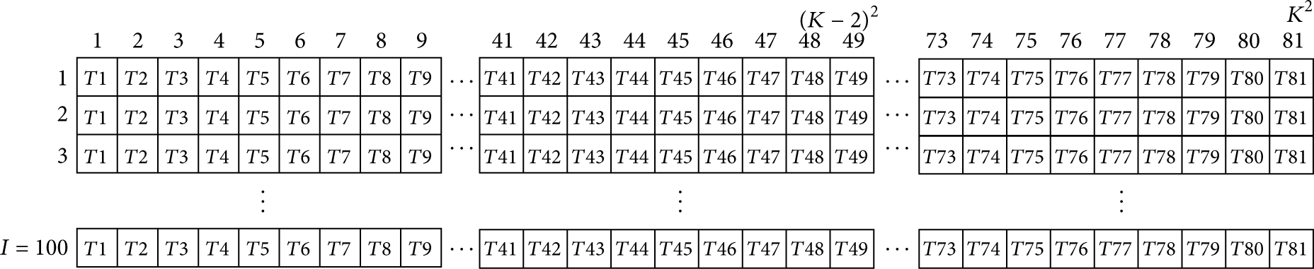
Global model-based arrangement from the calibration data, conformed by $I=\mathrm{100}$ observations of $J=\mathrm{81}$ variables each.

It is important to note that the actual location of a sensor in the data arrangement does not have any influence in terms of model calibration, monitoring, or data recovery.

5.2. Data Recovery: Local Modeling

Regarding the subsequent recovery procedure, TSR aims to restore the values affected by an attack or a sensor failure. This method, as mentioned before in Section 4, tries to impute the missing values through the available sensor measurements, so that the imputation accuracy increases as there exist more available unaffected values and they are correlated with the affected ones. Because of this last condition for TSR, the global modeling previously introduced is expected not to provide an optimal arrangement to derive our model, as not all the data values in the network area are correlated. For this reason, a different arrangement of the WSN data for missing data recovery is proposed. We consider in this case only the sensors located in the vicinity area surrounding an attacked sensor. The PCA or PLS model calibrated from this arrangement of the data is referred to as a local model. We will see how this affects the recovery performance in Sections 6.3 and 7.

A main concern in the calibration of local models is how to arrange the data when the sensors are not regularly distributed in the sensor field. Figures 5 and 6 depict the arrangement process to build up a local model for PCA and PLS for regular and nonregular topologies, respectively. In both cases, the vicinity of a given sensor is defined by its closest neighbor sensors (in Figures 5 and 6, eight neighbors are considered). Each neighbor is represented by an arrow indicating the relative position to the affected sensor for the regular topology and by an identifier in the nonregular topology case (they are numbered in order of distance, from the closest one, 1, to the farthest one, 8). We discuss in Section 8.3 how a value other than 8 for the vicinity affects the recovery results.

Figure 5

Local model for a regular topology of the sensor field. The locality illustrated is established to 9 sensors, so that the total number of observations is $I\times (K-\mathrm{2}{)}^{\mathrm{2}}$ , where I is the number of original observations and K is the number of sensors per side, $(K-\mathrm{2}{)}^{\mathrm{2}}$ being the number of sensors considered. In this structure z corresponds to the last sensor value at the Ith original observation.

Figure 6

Local model for data arrangement for a nonregular topology of the sensor field. The locality is established to 9 sensors, so that the total number of observations is $I\times J$ , where I is the number of original observations and J is the number of sensors. In this figure m corresponds to the last sensor value at the Ith original observation.

A measure of each target sensor and its neighbors (i.e., the locality is $\mathrm{9}$ -dimensional) is acquired every sampling time, which constitutes an observation in the local model. For a regular network, we only consider the $(K-\mathrm{2})\times (K-\mathrm{2})$ inner sensors to build the local model. Thus, X is $I·(K-\mathrm{2}{)}^{\mathrm{2}}\times \mathrm{9}$ -dimensional. On the other hand, for nonregular network, defining locality or vicinity is not a trivial task. The following procedure is proposed for that, where we consider that the position of each sensor is known or at least estimated with a certain accuracy:

• (i)

For a given sensor, its 8 closest neighbor nodes are obtained using the Euclidean distance (Figure 6).

(ii)

To conform the local model, each $\mathrm{9}$ -dimensional observation is obtained by combining the value of the target sensor with those of its 8 closest neighbors. It is important to note at this point that the neighbors are arranged in a specific order. For instance, in PCA the value of the target sensor is inserted between the nearest four and the farthest four sensors, thus conforming the matrix X. The order is not relevant itself but all the observations should follow the same order. In the PLS case, there exist two separate matrices, X and Y. The first one contains all the variables (sensors) except the target one, which is located in the Y matrix and whose values are estimated by using X.

In order to clarify the local model building, take the case in which we have $J=\mathrm{81}$ sensors, $I=\mathrm{100}$ observations of each of them, and $K=\mathrm{9}$ sensors per side corresponding to the regular sensor field. Figures 7(a) and 7(b) specify the new locality-based arrangement resulting for PCA and PLS, respectively. As indicated, we make use of 9 sensors (the affected one and its 8 closest neighbors) and $I=\mathrm{100}$ observations. Therefore, we have $(K-\mathrm{2}{)}^{\mathrm{2}}=\mathrm{49}$ inner sensors and the dimension of the local model is 4900 × 9 for PCA, being $4900\times 8$ in X and $4900\times 1$ in Y for PLS.

Figure 7

Local model arrangement for (a) PCA and (b) PLS from the global model shown in Figure 4 in which there exist $I=\mathrm{100}$ observations, $J=\mathrm{81}$ sensors, and $K=\mathrm{9}$ sensors per side in the regular sensor field.

6. Simulation Scenario: Regular Sensor Network

In most WSN-related environments, the CU gathers and analyzes the measurements generated by the sensors over time. The present work is focused on data collected this way for a critical environment like military actions, crisis management, or disaster recovery [2]. In particular, we focus our study on a fire fighting scenario in a forestry area. The main reason for this choice is the social and economic relevance of this kind of environments at present. Using this simulated environment, normal temperature conditions and fire situations will be simulated, as well as several specific data tampering attacks. Upon such a scenario, an anomaly detection system based on multivariate analysis is used to alert a human supervisor when an anomaly occurs. This supervisor is in charge or discerning between actual fire situations and malicious attacks, aided by the visualizations in the multivariate monitoring system. If an attack is determined, a subsequent recovery process is launched to restore the original sensor values affected by the attack.

We will analyze the effects of the attack, the performance of our recovery scheme, and how they depend on the specific routing algorithm implemented in the network.

6.1. Framework Description

Some WSN simulation tools are useful for experimentation [35]. However, most tools mainly focus on network features (e.g., physical layer, protocols, and propagation models) and usually ignore the environmental situation and real physical magnitudes. For this work we have developed a specific simulator based on Matlab 2009b to obtain the temperature evolution of a forestry area. It is inspired by [36], where the authors present a model in which the temperature obtained by a given sensor is calculated by including the contribution of close fire focuses. A fire focus is modeled using a 2D Gaussian distribution, which is used to simulate the temperature acquired by a sensor under normal conditions and under a fire situation. Figure 8 shows the simulation scenario, where Figure 8(a) corresponds to the distribution of the sensors in the area. Two types of temperature maps are also presented. Derived from normal conditions, Figure 8(b) shows three normal temperature (in °C) sources representing the hottest areas, which may be valleys, among cooler zones representing mountains. Figure 8(c) illustrates a fire situation where the fire has a central focus covering more than half of the total area.

Figure 8

Simulation scenario: (a) sensor locations, (b) temperature map under normal conditions, and (c) temperature map with a fire focus.

We assume a 1000 m × 1000 m square area of forestry where 81 ( $9\times 9$ ) sensors are regularly distributed; that is, each sensor is located ~100 m away from its neighbors (Figure 8(a)). Every sensor acquires the ambient temperature for predefined sampling times and sends the measurements to the CU. The proposed deployment for the measurements is inspired in a real system provided by Libelium company (http://www.libelium.com/wireless_sensor_networks_to_detec_forest_fires/).

The simulation tool is first employed to generate a data set used to calibrate a PCA model (hereafter, CAL data set). The data matrix X contains 100 observations of 81 variables (the temperatures obtained by each sensor) under normal temperature conditions, that is, without a fire situation. A situation in which a fire focus evolves over time is then simulated (hereafter, FIR data set). These data sets are used to study the detection capabilities of our anomaly detection system.

To evaluate the capacity of the PCA-based model against certain attacks, three variants of a data tampering scenario are simulated (hereafter, ATA data set). They differ in the specific routing algorithm considered in sending the sensor data to the CU. First, a direct communication between each sensor and the CU is assumed using the general packet radio service (GPRS). In this case, the tampering of a sensor only affects the measurements collected by that sensor. This situation corresponds to what is hereafter called an isolated attack, illustrated in the upper left part of Figure 9. Second, a more severe attack can occur in a multihop routing scheme, where just attacking a single sensor would affect all previous sensors in the route. The bottom part of Figure 9 illustrates this attack for a linear (left-to-right) routing scheme, which is inspired in the MCFA routing protocol [1]. This is hereafter referred to as the line attack. More sophisticated routing schemes may be also considered for WSNs. LEACH [1] is a well-known routing algorithm designed to reduce energy consumption by arranging the sensors in clusters, so that the so-called cluster head (CH) performs data aggregation prior to sending the collected data to the CU. Figure 10 depicts a scenario in which a CH is compromised, affecting all the sensed values in the cluster. This is hereafter referred to as the cluster attack. Notice that although the names isolated, line, and cluster attack are used for the sake of easy understanding, in all the cases we consider that a single sensor is being tampered. Thus, they should not be understood as different variants of a tampering attack but as different consequences of the same attack due to the routing scheme being used in the WSN.

Figure 9

A malicious node modifies the values of a single sensor, which can affect the values corresponding to one (isolated data tampering) or more sensors (line data tampering).

Figure 10

A malicious node modifies other sensor values during the data aggregation process (cluster attack).

Each tampering scenario variant considered (i.e. isolated, line, and cluster) is introduced in a separated test set where the evolution of a fire is simulated over time. The goal of the validation study performed is twofold: (a) to analyze the capability of the proposed PCA-based system to determine the occurrence of tampering attacks and (b) to be able to recover tampered data in order to restore the normal functioning of the environment and to enable the correct operation of the fire brigades for optimal positioning and strategy making.

6.2. Monitoring and Anomaly Detection

We use the PLS-toolbox in the Matlab environment [37] to illustrate the proposed approach for WSN monitoring. Firstly, the number of PCs has to be selected in PCA. There is no perfect solution to determine the number of PCs when the model is used for monitoring [30]. The inspection of the eigenvalues showed that 1 PC is an adequate choice. By comparing the PCA model obtained from calibration to the new observations under monitoring (i.e., the test data set), anomalies in the environmental behavior are detected. This detection is performed through monitoring graphics such as those presented in Figure 11, in which the $T^{\mathrm{2}}$ statistic is the abscissa and the Q statistic the ordinate. Each sampling time, a new observation is collected from the WSN and the scores are computed (see (2)) and the statistics $T^{\mathrm{2}}$ and Q obtained (see (8) and (9), resp.). A point in the plot represents one sampling time in the WSN. The Figure 11 points out the sampling times corresponding to the fire evolution (inverted triangles) in the ATA data set as anomalous events, because they differ from those corresponding to normal conditions (dark circles) in the CAL data set. The monitoring system automatically triggers an alarm when the monitored behavior deviates from the normal operating conditions established from the calibration data. This occurs when the control limits of the statistics are exceeded for three consecutive sampling times (three consecutive sampling times are commonly used in typical multivariate statistical process control (MSPC) deployments). In the system proposed, the control limits are chosen such that 95% of the observations gathered in the calibration stage fall below the limits. This means that the theoretical probability for false positives is 0,05³ = 0,000125. According to Figure 11, the monitoring system can detect the fire situation (inverted triangles) from the beginning of its evolution.

Figure 11

Monitoring graphic: initial calibration data (dark circles) and control limits (dashed lines), from which anomalies are detected (inverted triangles). Q contribution plot detailing anomalous specific observation (top left).

It is also important to remark that at this point the monitoring system is not capable of automatically distinguishing between actual anomalies, such as fire events, and false alarms caused by a potential tampering attack or a sensor malfunction. In other typical PCA/PLS monitoring schemes, such as in industrial process monitoring [33], there exists a human supervisor who distinguishes between real anomalies and false alarms. To aid this supervisor, contribution plots are issued after an alarm is triggered. We inherit this approach in our proposal.

Figure 12 shows the typical pattern for the Q contribution in the fire case, while Figures 15(a), 15(c), and 15(e) show the patterns obtained under attack (isolated, line, and cluster, resp.) in the same fire scenario. The tampering attacks are shown as sharp artifacts which depend on the routing scheme and which are clearly different to the smooth contribution of a true fire.

Figure 12

Q contribution plot for a fire situation (FIR data set).

Although the human intervention can be seen as a shortcoming of the proposed approach, the relevance of fire detection requires such an intervention in a practical system. The automation of the distinction between real anomalies and false alarms is out of the scope of this paper. However, a tentative approach is illustrated here inspired in filtering methods of image processing [38]. Filtering methods can be used to highlight specific artifacts in a plot. Thus, they can be used to highlight the artifact generated by a tampering attack for a given routing. For instance, if a line routing scheme is being used, a filtering window to detect lines can be employed, as shown in Figure 13. Once the filtering window is applied to the contribution plot, we can see a considerable accentuation of the line affected by the attack. Afterwards, a threshold can be established to distinguish between artifacts and actual anomalies.

Figure 13

Q contribution plot after a window filtering process for the line tampering attack shown in Figure 15(c). This filter accentuates the attack for a subsequent threshold-based automatic detection. The line sensor accentuated by the filtering process is highlighted by a dashed circle.

Whatever the detection method, either manual or automatic, used to determine the occurrence of false alarms due to tampering or malfunction, a missing data recovery process is afterwards executed to solve the situation and recover the affected data. This process is discussed below.

6.3. Missing Data Recovery

After an attack detection alarm, a response mechanism should be performed to mitigate the consequences of the threat and achieve the system survivability. A main contribution of the present work is to treat the detected “fraudulent” values as missing values and estimate them using missing data recovery techniques.

First of all, the global model used for monitoring will be employed for data recovery. To select the optimal number of PCs, we use the cross-validation method mentioned in Section 3.3 and the PRESS shape. Figure 14 shows that 3 PCs seems to be an adequate number of PCs, since the PRESS attains its minimum value for that number. This number agrees with the fact that the CAL data set has exactly three variability sources, corresponding to the temperature focuses.

Figure 14

Cross-validation PRESS curve for the simulated data set considering the global model.

Figure 15

Simulated data tampering: (a) profile generated from the fire situation in Figure 12 and an isolated attack and (b) recovery results after the imputation process; (c) profile generated from the fire situation in Figure 12 and a line attack and (d) recovery results after the imputation process; (e) profile generated from the fire situation in Figure 12 and a 3 × 3 cluster group affected by the attack and (f) recovery results after the imputation process. In each figure, those sensors affected by the associated attack are highlighted with a dashed circle.

Once we got the optimal number of PCs for our specific CAL data set, we can evaluate in optimal conditions the TSR-PCA missing data imputation method for the three mentioned data tampering cases: isolated, line, and cluster. Figures 15(b), 15(d), and 15(f) represent the result of each corresponding attack after the data recovery process. The Q contribution is smoother after data recovery than the original cases in Figures 15(a), 15(c), and 15(e). However, the results are far from being optimum. The Q contribution for distant sensors from the fire is lower than that for closer sensors, in which a greater Q contribution is exhibited. This is because we have estimated the PCA model for normal conditions (without fire), while data tampering experiments are performed under fire circumstances. The recovery from data tampering attacks in distant locations from the fire is more effective. Such circumstance can be observed in Figures 15(d) and 15(f), where the values of the sensors closer to the fire focus are not correctly restored.

Beyond the visual-based results, Table 1 shows numerical results of the recovery using the mean squared error (MSE) between actual and restored data. To avoid the aforementioned sensors location influence on the results, we calculate the average MSE value for all sensors in the $9\times 9$ network. This is performed by repeating each of the tampering cases (isolated, line, and cluster) so that each of the $9\times 9$ sensors in the network is tampered and recovered once.

Table 1

MSE comparison for different tampering attacks using TSR-PCA as missing data imputation method.

Data tampering	MSE (TSR-PCA)
Isolated	1900.8
Line	2472
Cluster	4391.6

The isolated data tampering has the lower MSE because the recovery method has more available valid data to recover the sensor values affected by the attack. The worst case corresponds to the cluster attack, where most sensors in the neighborhood of the tampered one are also affected and can not be used in the recovery. In the line case, each tampered sensor has at least one sensor below and above it with valid data to allow a better recovery than in the cluster case. In summary, the routing algorithm is a key aspect to consider in this problem. Although an aggregation algorithm is a good choice from an energetic perspective, it may be not from a security perspective using imputation methods.

In order to complete the previous results we also study the evolution of the MSE as a function of the fire progress as well as of the number of tampered sensors. The results are presented in Figures 16 and 17, respectively. In the first one, we depict the MSE evolution for the 10 first sampling times from the beginning of the fire. We can observe a clear incremental evolution of the MSE. Also, in accordance with the results in Table 1, the isolated attack presents the lowest MSE trend while the cluster attack doubles this trend. In Figure 17, we show the MSE evolution with the number of tampered sensors in the isolated case in which the numbers of tampered and affected sensors match. The results are obtained by randomly tampering from 1 to 10 sensors. We can see an increasing MSE evolution with the number of sensors tampered. This increasing behavior is the consequence of randomly selecting adjacent sensors, so that the missing data imputation technique has less available sensor values to infer the original values of the tampered sensors. Still, the tendency shows a linear profile with low multiplicative constant, so that the increase in the number of tampered sensors sevenfold only doubles the MSE.

Figure 16

Evolution of MSE for the 10 first sampling times with the presence of fire considering global models and for each data tampering case (isolated, line, and cluster).

Figure 17

Evolution of MSE with the presence of fire considering several tampered sensors for global models by using the isolated routing strategy.

7. Improving the Missing Data Recovery Performance: Local Modeling Approach

Instead of using all sensors for data imputation as in the case of the global model presented in Section 5.1, the local modeling approach is used in this section (see Section 5.2 for details) where only the sensors closest to the affected one are considered to recover the missing values. The local model is only used for imputation, not for monitoring purposes where the global model is still considered. Two models are thus involved: the global model for data monitoring and a local model for data imputation.

The optimum number of PCs for a local model must be estimated again as it was in Section 6.3 for global modeling. According to Figure 18, the lowest PRESS value is obtained for 7 PCs in both PCA and PLS cases.

Figure 18

Cross-validation PRESS curve for the simulated data set considering the local model. The lowest PRESS value is obtained for 7 PCs in both cases: PCA and PLS.

To compare the recovery results obtained by using global and local models, the MSE and Q contribution plots are obtained. Figure 19(b) shows the Q contribution after data recovery for the isolated attack. It clearly outperforms the imputation provided by the global model in Figure 15(b), and it resembles with high fidelity the case in which no attack exists (Figure 19(a)). A similar conclusion is obtained from the MSE values in Table 2. Analogous results and conclusions can be extracted for line and cluster attacks in Figures 19(c) and 19(d), respectively. The same occurs with the corresponding MSE values in Table 2.

Table 2

MSE for local model-based TSR-PCA and TSR-PLS missing data imputation methods.

Data tampering	MSE (TSR-PCA)	MSE (TSR-PLS)
Isolated	2.6506	3.4036
Line	67.7999	71.085
Cluster	149.5746	148.7155

Figure 19

TSR-PCA data tampering imputation through local modeling: (a) original profile for the fire, (b) sensor imputation for isolated attack, (c) sensor imputation for line attack, and (d) imputation for cluster attack. Those sensors affected by the associated attack are highlighted with a dashed circle.

In summary, results in Tables 1 and 2 demonstrate the benefits of using local versus global modeling for data imputation. The new arrangement method can significantly reduce all MSE values. In the isolated case, a reduction of 99.86% is achieved, while the reduction is 97.25% in the line case and 96.61% in the cluster case. Both TSR-PLS and TSR-PCA missing data imputation methods provide similar results because the number of latent variables is chosen in both cases using the same method: cross-validation (Section 3.3). Thus, they are working in optimal conditions for missing data imputation.

We also explore the evolution of the MSE as the fire evolves in Figure 20 in a similar manner to Figure 16 for the global model case. In addition to the incremental evolution of the MSE value observed again, the improvement provided in the estimation performance by local models is clear. This behavior can be explained by the fact that the global model is more sensible to fire. That is, the sensors affected by the fire focus are included together with those far from it in the model, which leads to the estimation of the value of sensors using other sensors in different conditions. In a local model, instead, the sensors considered are limited to the neighborhood, so that a sensor affected or not by fire is estimated from sensors under the same conditions.

Figure 20

Evolution of MSE using the 10 first sampling times with the presence of fire considering local models and for each data tampering case: (a) isolated data tampering, (b) line data tampering, and (c) cluster data tampering.

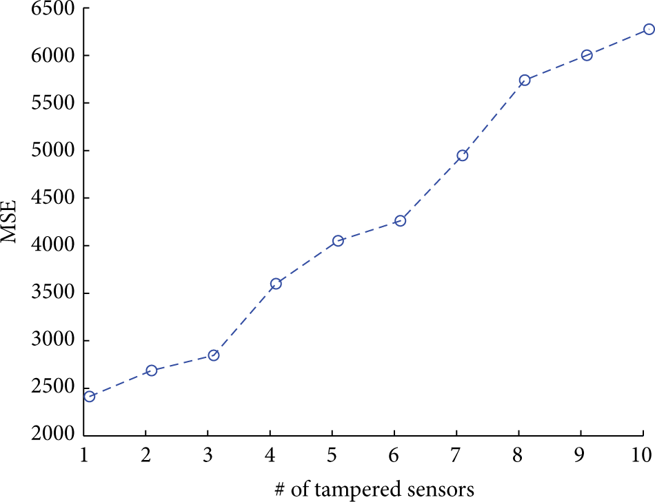
Finally, we study the MSE evolution as a function of the number of tampered sensors. This is shown in Figure 21. As in the global model case (Figure 17), the MSE grows with the number of tampered sensors. Again, we find a linear increasing behavior. In this case, the multiplicative constant is higher showing that randomly chosen adjacent nodes have a deeper impact on the local model performance. Still, the MSE of local models is several orders of magnitude lower than that of global models.

Figure 21

Evolution of MSE with the presence of fire considering several tampered sensors for local models by using the isolated routing strategy.

We can conclude, from the previous discussion and results, than our proposed missing data imputation method plus the local data arrangement leads to a high recovery performance even with adverse conditions: dynamic environmental changes (fire evolution) and a reasonable number of sensors tampered (around 12% of the total). Consequently, the proposal improves the robustness of WSNs against security threats and so its survivability.

8. Real Scenario: LUCE (Lausanne Urban Canopy Experiment) Deployment

In this section, a real WSN scenario is used to corroborate the validity of the results obtained in simulation.

8.1. Sensor Deployment Description

LUCE (Lausanne Urban Canopy Experiment) (LUCE deployment data set at http://lcav.epfl.ch/page-86035-en.html) is a WSN project driven at the EPFL (École Polytechnique Fédérale de Lausanne) campus since July 2006. This is an innovative system that allows for the first time studying the interactions between an urban environment and the lower atmosphere.

LUCE aims to better understand micrometeorology and atmospheric transport in urban environments. The system is based on a wireless sensor network of 100 SensorScope weather stations that are deployed on the campus (about 500 m² area). These stations measure key environmental quantities at high spatial and temporal resolutions.

Each SensorScope weather station has several sensors. Among others, there are ambient temperature, humidity, and wind speed sensors. These measures are acquired and sent for analysis via GPRS to a CU with a periodicity of 30 seconds.

Table 3 compares the features of the simulation environment and the LUCE data set. Both have a similar deployment area and a similar number of sensors, and both consider temperature measurements. Despite these similar characteristics, they refer to two completely different scenarios, as LUCE provides measurements corresponding to a real environment. This way, we argue that LUCE constitutes a valid “test bed” to definitively conclude the applicability of our approach.

Table 3

Simulation scenario versus LUCE real deployment scenario.

Scenario	Characteristic	Value
Simulated	Area (m2)	1000
	Number of sensors	81
	Ambient temperature sensor	yes
	Other sensors	no
	High temporal & spatial density	yes
LUCE	Area (m2)	500
	Number of sensors	100
	Ambient temperature sensor	yes
	Other sensors	yes
	High temporal & spatial density	yes

Data collected from November 2006 to May 2007, available from the LUCE project web site, are used in this paper. We have chosen data between January 1 and January 31, 2007, for our experiment because this corresponds to the most complete time interval, with 80,000 ambient temperature samples per sensor. The number of sensors used in our study is 61. Figure 22 shows the location of these 61 sensors, specifying the latitude and longitude coordinates. Also we show the 8 closest sensors to a given one (sensor with ID = 100).

Figure 22

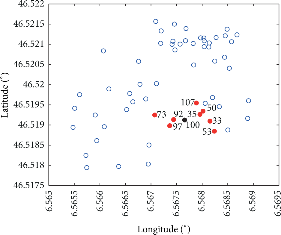
Location of the 61 sensors in the LUCE deployment used in our experimentation. As an example, we show the 8 closest sensors to a given one (sensor with ID = 100).

8.2. Anomaly Detection and Data Imputation with Global Models

The same monitoring method developed in Section 6.2 is deployed for LUCE. The first twenty days of the previously mentioned data range are chosen as the calibration set to train the PCA model. The remaining days are used for testing purposes. The daily average value is subtracted from the data of the corresponding day to correct for temperature drifts along days.

Figure 23 shows the calibration model, after outliers isolation, as dark circles. After establishing the control limits, all subsequent observations (inverted triangles) are classified as normal, except the one in a dashed circle (top left), which corresponds to an artificially generated anomaly for the present work.

Figure 23

Monitoring graphic: initial calibration model (dark circles), control limits (dashed lines), and subsequent observations (inverted triangles) classified as “normal” events, except the one in a dashed circle (top left), which corresponds to an anomaly.

Note that there is no fire influence in this case. Therefore, an anomaly could be produced either by data loss or by a device malfunction. These anomalies, as in the WSN simulated case, can be deduced from the Q contribution graphics. Figure 24 shows that the Q contribution presents a significant deviation for a specific sensor that was actually tampered for the experiments.

Figure 24

Isolated tampering Q contribution. Those sensors affected by the associated attack are highlighted with a dashed circle.

After detecting the anomaly, a TSR-PCA-based missing data recovery method is used as a response mechanism, as indicated in Section 6.3. Figure 25 shows the recovery results obtained when using global modeling. Numerical (MSE) results are also provided in the second column of Table 4.

Table 4

MSE comparison between global and local models.

Data tampering	Global model	Local model
	MSE (TSR-PCA)	MSE (TSR-PCA)	MSE (TSR-PLS)
Isolated	0.1051	0.1081	0.1030

Figure 25

Missing data recovery results applying the global model. The sensor affected by the associated attack is highlighted with a dashed circle.

No routing algorithm is used in the LUCE experiment, as data from sensors are directly sent via GPRS to the CU.

8.3. Local Models for Nonregular Locations

Using local models for data imputation in regular and equally distributed sensors environments is straightforward, as the 8 closest sensors to a given one are those surrounding the latter. Defining the number of closest sensors in nonregular scenarios is not such an easy task. Therefore, a method to determinate this number is needed. To address this issue, we get the MSE values by varying the number of closest neighbor sensors selected in the local model to carry out the data imputation/recovery procedure. The results obtained are depicted in Figure 26. We can see that the optimum number of neighbor sensors is around 6–8, while considering a higher number of sensors provides similar MSE values. In consequence, and for the sake of comparison with the regular scenario, we also choose the 8 closest sensors to carry out the missing data recovery process in the real nonregular topology scenario.

Figure 26

MSE evolution with the number of sensors considered as valid values for the missing data imputation method.

Also, a remarkable aspect is the distribution of the closest sensors around an affected one. If most of the closest sensors are distributed in a nonhomogeneous way around the manipulated one, the prediction accuracy is expected to be worse than in the case that they are located in a regular way surrounding the affected one. This way, we have some prediction uncertainty depending on two main factors: the distance of the closest sensors to the tampered one and their distribution around it. This should be addressed in future works.

The data imputation results obtained for LUCE when using local models are visually similar to those obtained in Figure 25. Table 4 shows the associated MSE values. In this case, similar results are obtained to those with global models, mainly because a high spatial correlation exists in the LUCE data set such that almost all sensors are highly correlated. To corroborate the existence of this high correlation, we calculated the correlation coefficients between variables, $\mathrm{0.89}$ being the minimum value found.

Another interesting experiment may be useful to assess the robustness of the imputation approach when more than one sensor is compromised. We sequentially increase the number of tampered sensors from a selected one to its closest 8 sensors. For example, 1 means that only a sensor is tampered, the selected sensor, 2 means that we tamper the specific one and its closest neighbor, and so on until 9 sensors in total. Figure 27 illustrates the evolution of the MSE parameter with the number of tampered sensors. The MSE value does not vary significantly when the number of affected nodes is lower than or equal to 7.

Figure 27

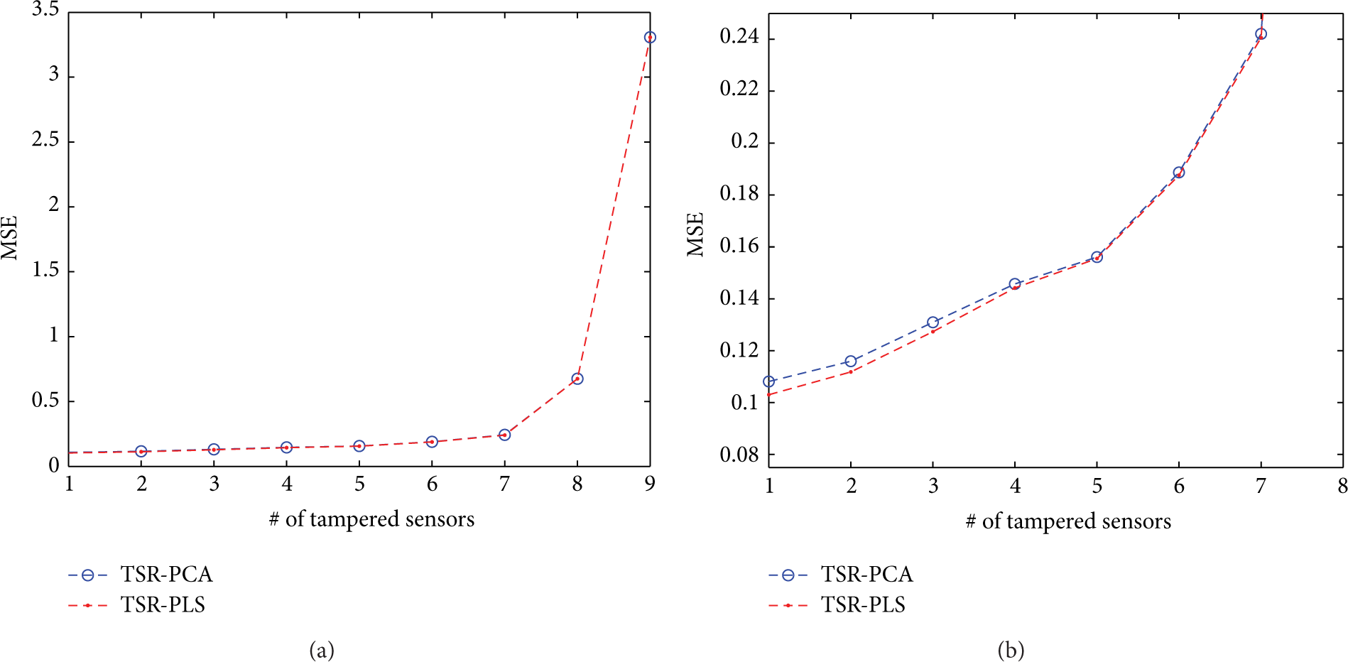
MSE evolution with the number of tampered sensors: (a) 9 tampered sensors; (b) zoom for only the first 7 tampered sensors.

9. Conclusions and Future Work

This paper introduces the use of multivariate analysis techniques for anomaly detection and data loss/modification identification and recovery in wireless sensor environments. Both multivariate proposals, that is, anomaly detection and data imputation, are tested using a temperature-related experimental study that considers simulated and real environments.

As an additional contribution, we have shown that different routing algorithms may amplify the harm of the data loss in a different way. In particular, by properly selecting the routing algorithm, data loss due to a tampering attack or sensor malfunction can be better detected and lost data can be better recovered.

Two types of models for data recovery are assessed: global and local models. The latter achieve better performance when a higher correlation exists between sensor values in the neighborhood of a given affected/attacked node.

The promising results obtained suggest extending the study to other types of attacks, including dropping or delay attacks, and exploiting the temporal correlation among measurements. Moreover, as the routing algorithm influences missing data recovery results, the design of efficient routing algorithms to preserve the network correlation information is also an interesting future research line. Another relevant issue is that of potentially faking the node location information. The proposed data recovery process relies on neighborhood information, while the actual vicinity of such nodes is not checked. In future versions of our scheme this aspect should be also addressed.