Sage Journals: Discover world-class research

Abstract

Time synchronization is a crucial part of distributed systems. It is often required for data reliability and coordination in wireless sensor networks (WSNs). Wireless sensor networks have three major goals: time synchronization, low bandwidth operation, and energy efficiency. Different time synchronization algorithms are aimed at achieving these objectives using various methods. This paper presents performance evaluation of two state-of-the-art time synchronization protocols, namely, Flooding Time Synchronization Protocol and Recursive Time Synchronization Protocol. To achieve time synchronization in wireless sensor networks, these two protocols make use of broadcast and peer-to-peer mechanisms. Flooding Time Synchronization Protocol uses the former mechanism, while Recursive Time Synchronization Protocol uses the latter mechanism. To perform the performance evaluation, three performance metrics are used including synchronization message count per cycle, bandwidth, and convergence time. Arduino is used as a micro-controller and XBee as transceiver to verify these metrics by utilizing different topologies.

1. Introduction

In recent years, significant advances in technology have emerged following the creation of low-cost sensors for processing and communicating data [1]. Wireless sensor networks (WSNs) are a type of distributed networks wherein sensors are launched to monitor real-time occurrences. Sensor nodes can be deployed into various types of environments and can be static or mobile. Once deployed, they begin the process of discovering an entire network for communicating the data collected individually [2]. There are numerous applications of WSNs that ranges from medical [3, 4], environmental [5, 6], military [7], industrial, civilian, vehicular [8], microclimate studies [9, 10], and water pollutant monitoring [11], to urban hazard avoidance [12], interplanetary communication [13–15], sensor web probing [16], navigation [17], and home networks [18, 19].

Although conventional sensing architecture is not appropriate for these applications, they work well in unobstructed environments such as sky observations via weather radars [20]. They consist of a few sensors that are high-powered and of long-range. In order for these sensors to communicate, they need a clear line-of-sight. However, these are not effective in harsh, disordered, and complicated environments, where visual contact is limited. Many short-range sensors decrease the clutter effect. This pattern of sensors similarly develops a signal-to-noise ratio, which is vital to sensing phenomenon. However, it is not practical to utilize wired sensors in large areas, because they involve appropriate infrastructure. Manual observation is also labor and time intensive. Hence, using conventional sensing architecture is considered insensible for these types of applications.

Utilizing time synchronization in WSNs renders it vital; however, it is not easy to solve. Prerequisites for applications vary in precision, energy, lifetime, and availability. A case in point concerns global queries that necessitate global time and local collaboration that usually needs synchronization between at least two or more neighbors. Some sensor tasks might operate in an hourly or daily time scale, while acoustic applications operate at a microsecond's level and oftentimes require precision. Meanwhile, triggers may simply need momentary synchronization, even as data logging or debugging needs a time scale that is always constant. User communication needs coordinated universal time or other external time scales, while for the entire in-network appraisals need relative time only. Nodes also differ, because some are equipped with large batteries to enable them to run continuously and others are limited in their capacity. Limited in power nodes require to intermittently wake up to do single sensor readings, communicate, and then go back to sleep mode.

It is challenging to design a time synchronization that fulfills many requirements, especially for sensor networks. Apart from the aforementioned prerequisites, they also exhibit energy efficiency and automatic adjustment to scalability and dynamics. For example, limited energy [21] disrupts the rules established by the conventional algorithms of time synchronization. When the CPU is inactive, it only uses a small amount of energy, and the same applies to random transmissions that have minimum impact.

In this paper, real-time performance evaluation of two time synchronization protocols is presented, namely, Flooding Time Synchronization Protocol (FTSP) and Recursive Time Synchronization Protocol (RTSP). Both of them are tested in real-time environment using four different topologies, including bus, grid, mesh, and tree. Average messages per synchronization cycle, bandwidth, and convergence time are used as metrics for performance evaluation. FTSP is much simpler protocol as compared to RTSP, but RTSP can achieve better time synchronization at edge nodes in contrast to FTSP. The motivation for selecting these protocols is that FTSP is the benchmark of synchronization protocols. On the other hand, RTSP is a novel synchronization protocol developed by our research group. Our goal is to compare these two protocols in real-time.

Section 2 provides the related work. Section 3 discusses the hardware setup and limitations. Section 4 describes the implementation details. Section 5 presents and discusses the achieved results. Finally, Section 6 provides the conclusion and the proposed future work.

2. Related Work

Several protocols are proposed to synchronize physical clocks in computer and sensor networks [22–24]. Some of them are probabilistic clock synchronization [22], the network time protocol [25], optimal clock synchronization [26], slow-flooding time synchronization [27], a maximum value-based times synchronization [28], and distributed time synchronization protocol [29]. Following are the common characteristics of these protocols: (1) message exchange which involves the utilization of user datagram protocol, (2) the presence of one or more servers, (3) the timing information exchange among clients, (4) set-up approaches in case of error recovery during processing and transmission, and (5) using a client algorithm and master server information to update the clock. Some differences are also noted, such as whether the network is internally or externally synchronized with a clock, that is, whether a master server is used as the intermediary of client clocks or as the only clock.

The Reference Broadcast Synchronization (RBS) protocol uses wireless medium as its broadcast mechanism [30], as its name suggests. RBS uses wireless communication medium to receive broadcasted data simultaneously. To paraphrase, a group of receivers can receive the same data with only a little difference in delay. This message can be utilized for clock synchronization. Thus, each receiver logs the time stamp at which the message is received and compares it against its local clock and then updates its local clock accordingly. All receivers within the proximity of the transmitter can synchronize with high accuracy. RBS uses multiple synchronization messages to calculate both skew and offset of the local clock relative to one another. RBS exploits another concept called time critical path. Time critical path is defined as the path of the message that contributes to nondeterministic errors in the protocol. Some additional features are (1) no clock correction: once clocks are synchronized, that is, skew and offset are calculated, nodes local clocks are not synchronized with global clock, (2) post facto synchronization: RBS conserves high level of energy, because it is synchronizing clocks when the event of interest occurs, so nodes switch to power saving mode at other times when there is no event of interest, and (3) multihop communication: RBS uses an intermediate node to synchronize two nodes that are situated at different ends; otherwise, it will lose accuracy due to delay in broadcast message reception. RBS has several advantages; for example, skew and clock offset are calculated independent of one another. Post facto synchronization conserves energy on the expense of clock updates, and multihop communication is supported and it can maintain both clocks (relative and absolute). On other hand, RBS has some drawbacks such as the fact that it is not suitable for point-to-point network communications and it requires O ( $n^{2}$ ) operations for message exchange in a single hop network of n nodes. Moreover, the convergence time is high. Moreover, if the reference node requires synchronization then a large number of messages will be exchanged, thus resulting in energy inefficiency.

Until recently, Flooding Time Synchronization Protocol (FTSP) [31] is the most widely used protocol for time synchronization among nodes. It employees broadcast mechanism to achieve synchronization objective. The reference node broadcasts the message containing timing information. Any nodes in its broadcast radius (RF coverage area) will listen to the message and update their local clocks accordingly. Reference node is elected dynamically and it broadcasts its timing information in predefined time interval. FTSP forms an ad hoc tree structure instead of fixed spanning tree. To eliminate the effect of random delays, medium access control layer time stamping is used at both ends. These time stamps are embedded into each message at the end of the start frame delimiter (SFD) byte, but this happens after correcting error and normalization of time stamp. Least square linear regression is used to estimate offset and skew of timestamps. After nodes local clock is synchronized with the global clock, it starts broadcasting timing information in the network. This way, the whole network is covered [32].

The Recursive Time Synchronization Protocol (RTSP) presented in [33, 34] supports multiple topologies, that is, flat, mesh, star, and cluster topology. Any node in the network can send time synchronization request. The request is forwarded in a recursive multihop manner to the reference node. The reply is sent via reverse path by the reference node. A node is elected dynamically and according to this node timing information, the network is synchronized. This node is also called root node or any synchronized intermediate node. Each node along the reverse path will compensate for time drift, that is, propagation delay. It also uses medium access control layer time stamping at both ends. These time stamps are embedded at the end of start frame delimiter (SFD) byte. There exist several algorithms that are proposed in RTSP like selection of reference node, cluster-heads, and working under different topologies [24, 29].

The following provides a brief description of RTSP protocol using an example. RTSP message consists of message type (enquiry/election (ERN), request (REQ), or reply (REP)), message ID, original source ID, intermediate source ID and destination ID. Let us assume that the request is sent from source $T_{1}$ and received at destination $T_{2}$ , the reply is sent at $T_{3}$ , and the reply is received at the destination node $T_{4}$ and reference time $T_{r}$ . The time drift is calculated and adjusted at each node along the reply path, using the following formula:

\begin{matrix} d = \frac{((T_{2} - T_{1}) + (T_{4} - T_{3}))}{2}, \\ T_{r} = T_{r} + d, \end{matrix}

(1)

where d is the time drift. This time drift compensates for the propagation delay. When the message reaches edge nodes, reference time becomes the same as on reference node [32].

3. Hardware Setup and Limitations

The hardware used for our implementation is 16 XBee RF modules, 16 XBee Shields, 16 Arduino Mega Boards, 15 9 v Batteries, and 1 XBee Explorer. Further details can be found in [32].

There are few limitations of above-mentioned hardware. XBee Pro has a proprietary implementation, thus limiting the implementation to only vendor provided functions. For instance, network or MAC layer cannot have custom functions/protocols implementation. Another very important problem with XBee Pro module is that it implements devices as a software application-programming interface (API), that is, for coordinator, router, and end device. We have a built-in API that can be loaded into the device. If these devices truly implemented Zigbee then we should be able to make the aforementioned network topologies easily, but this is not the case. Zigbee dictates the following: if two devices are configured as end devices then there should not be a direct communication between them, but that is not the case; even if the devices are configured as end devices, they are still able to communicate with each other that complicate things further. There are also some implementation issues when using Arduino and XBee. If several packets are coming, XBee might be able to receive all messages and transfer them to Arduino, but, due to complex programming at application layer, Arduino might not be ready to receive packets all the time. It might be busy in processing previous packet. Arduino can transfer six packets every second to XBee, but XBee cannot handle the packets at that speed. Therefore, to make it compatible with each other, we have to find an appropriate packet transfer rate between Arduino and XBee. This also puts an extra overhead in the implementation. XBee allows maximum packet size of 72 bytes, but it is not possible in our case to use all 72 bytes, because it cannot exchange 72-byte packet at the rate we are transmitting in our experiments. To utilize maximum packet size, there should be some delay between sending two packets. Packet size must be 50 bytes or less for efficient working of network. One very crucial problem relating to energy is that routers and coordinators cannot go to sleep, and their role cannot be changed dynamically. Thus, they require a constant energy source. Accordingly, energy efficiency aspect of both protocols cannot be analyzed using current hardware. Arduino also makes it hard to calculate energy utilization, because it does not provide functionality to calculate energy consumption. Another limitation of Arduino is that we cannot dynamically reply to the incoming message. We can read the network address from incoming packet, but, to reply dynamically, all the network address must be predefined in the software program [32].

4. Implementation

This section provides implementation details. Both protocols are simplified due to several reasons. One of the reasons is hardware limitation explained previously. Another reason is that some sections of the FTSP and RTSP algorithms are not relevant in current context, for example, energy compensation mechanism. We use time resolution in seconds, because it is not possible with the current hardware to use μs resolution for experimentation.

Due to hardware limitations, FTSP and RTSP algorithms are implemented at the application layer. All traffic came to application layer for processing. We could not utilize built-in functionality of lower layers, to simplify our implementation. For example, we had to implement duplicate message checking mechanism at the application layer rather than at the MAC layer, that already provides the functionality. This little function adds complexity and overhead at the application layer. There are also some implementation issues when using Arduino and XBee. If many packets are coming, XBee might be able to receive all messages and transfer them to Arduino. However, due to programming complexity at the application layer, Arduino might not be ready to receive packets all the time. It might be busy in processing previous packet. This also adds an extra overhead in implementation. Moreover, packet if we manually add delay in implementation at the application layer, Arduino. For example, if we specify at the application layer that a node should wait for 500 milliseconds between broadcasting two messages, this delay affects the rest of the node's functionality as well, for example, receiving a message and processing other instructions. To elaborate, a node is stuck at delay instruction, waiting for it to finish and the rest of the node's functionality is also halted. Almost identical code is embedded in all the nodes; therefore, it affects the whole network functionality.

Another technical issue with the implementation is nodes' power. All the nodes are powered up manually, which creates differences in the initial clock. Some clocks are ahead of others; this can lead to false root node selection, for example, if there are two nodes assigned IDs of 5 and 10. If we power up node 10 before node 5, then node 10 gets ahead start; therefore there is a high chance it becomes a false root node. With two nodes, it is possible to solve it easily. However, it is not easy to handle such situation manually when there are several nodes. Additionally, human error also contributes to this issue.

To avoid these technical issues and errors, the last node that powered up, immediately, broadcasts a reset message and other nodes reset their local clocks to zero state accordingly. Then, the process of root selection and time synchronization begins, thus eliminating any human errors.

Two types of messages are present in the network; (1) system messages (2) application messages. System messages are those that are used by XBee to communicate, such as routing messages or Ad hoc On-Demand Distance Vector (AODV) messages [35]. AODV is a broadcasting protocol used by XBee for routing. Therefore, it creates a broadcast path whenever it requires; however, these messages are hidden from the user. Users cannot interfere with these messages or modify them in anyway. The MAC layer checks for duplicate messages, but only for system messages not for application messages. On the other hand, application messages are being filtered at the application layer.

Metrics used for performance evaluation are message count, bandwidth, and convergence time. Total number of messages (incoming and outgoing) per synchronization cycle required for clock synchronization by each node is called message count. Any message received at the application layer is counted in message count metric. All protocols are implemented at the application layer and therefore duplicate messages come to application layer. Although duplicate messages are not processed with the exception to discarding, they are counted into message count metric. Second metric is the bandwidth. It is similar to message count because we multiply message size with message count; however, it is separated from message count. This is because, in some topologies, message count is low for one protocol, but bandwidth is high due to large message size. Thus, we need to distinguish between message count and bandwidth. Last metric for evaluation is the convergence time. It is the time required by an individual node for synchronization with root node. The reason for selecting these three specific metrics for performance evaluation is that bandwidth and convergence time are an important part of any computer networks. However, it especially holds true for wireless sensor network. Bandwidth consumption directly translates to the power consumption, which is a precious commodity in WSNs. Due to hardware limitations, we cannot compute bandwidth or power consumption directly, therefore we selected message count as our first metric that can be translated into bandwidth (message count × message size). Convergence time will measure, how quickly a node can resynchronize at the beginning or after a change in the network.

We implemented four topologies, that is, bus, grid, mesh, and tree. It was possible to implement all topologies using Zigbee; however, we experienced difficulties with XBee. Therefore, we formed these topologies manually. In other words, nodes were arranged into the required shape of the topology. As an example, for tree topology, nodes are arranged in a tree-like structure. The next section provides a detailed implementation of each topology.

4.1. Flooding Time Synchronization Protocol

Flooding Time Synchronization Protocol (FTSP) is simple and elegant protocol. It uses simple broadcasting mechanism for root selection and time synchronization. According to the work presented in [31], each Mica2 motes clock drift is 40 μs. To compensate for this drift, they implemented a clock drift mechanism. In our FTSP implementation, some simplifications are considered. There is no clock drift mechanism, because Arduino clock is accurate for approximately 70 minutes. Our experiments run for only 2.5 minutes, so there is no need for clock drift management. Because FTSP is a simple protocol, there is further simplification required. The following explains FTSP implementation with an example that includes root selection, root failure, and time synchronization.

Messages structure of the implemented FTSP is similar to that of FTSP messages. We implemented, a “nodeID,” “timestamp,” and “messageID.” One assumption that we made is that the network is connected. To ensure its validity, we wait for a fixed amount of time before broadcasting any message. In our implementation, the root node is a function of both time and nodeID. The node that has the smallest nodeID becomes the root node. In case of FTSP, there is no peer-to-peer communication; therefore, nodeIDs are assigned either dynamically or statically. After nodes are assigned nodeIDs, each node waits for predefined amount of time equal to its nodeID. The node that has the smallest ID number starts broadcasting timing information first; thus, becoming the root node. When root node broadcasts first synchronization message, it contains root nodeID, timestamp, and a unique messageID. Root node also adds this message to its message table for future duplicate message checking. All nodes in its radio range hear this broadcast message. Those nodes update their timing information, add this message to their message table, and rebroadcast the message without making changes. Message table contains all three parameters of the message. This message propagates to the end of the network. But, each node hears the message multiple times. If we do not discard the duplicate messages, these messages remain in the network until the end. To avoid infinite message loop, each node checks its message table whenever it hears a message. If the message exists, it increments the message count and discards the message.

In case of root node failure, if the nodes do not receive any messages within time T, they clear their root node. In other words, they reset everything and the same process is repeated. There is a minor chance of having two root nodes in the network, which is negligible. As it is mentioned previously, this is a simple broadcasting protocol with a simple message structure and reliable time synchronization method. However, the following issue does exist with this approach. As messages travel further away from the root node, there is no compensation for propagation delay, therefore edge nodes are not perfectly synchronized with the root node. To deal with this issue, RTSP utilizes request and reply mechanism.

4.2. Recursive Time Synchronization Protocol

Recursive Time Synchronization Protocol (RTSP) is complex and difficult to implement protocol. Backbone of the algorithm is request-reply mechanism for time synchronization. Request-reply mechanism guarantees propagation delay compensation at destination node. RTSP have three types of messages, that is, ERN, REQ, and REP. ERN messages are used for discovery and root selection, REQ are used for time request messages, and REP are used for reply messages. There are several other mechanisms employed by RTSP, for example, root selection, failure recovery, energy compensation, and clock drift management. We have simplified these protocols due to hardware limitations. The following provides our implementation details for RTSP.

RTSP is implemented at the application layer as well, and it requires peer-to-peer communication for accurate synchronization. However, it is not possible to dynamically determine the address of incoming message node and reply to that address using Arduino and XBee. In our RTSP implementation, root selection is a function of time and nodeID. In this case, we cannot assign nodeIDs dynamically. This is because we need to reply to each node directly rather than via broadcast method. In addition, reply message needs to follow the same path as of request message. Thus, each node has a complete table of all the nodes IDs and their corresponding network addresses.

In our case, root selection is a static process. Thus, this eliminates some complexity but creates another problem. In the original protocol after root selection, all nodes of the network know the root node. However, in our case, the process is static and nodes do not know which node is the root node. Nodes know the root node only after their timers are expired and the root node transmitted the message. For this protocol to function, we need a request and a reply message. There are several ways to solve this problem. We used a simple approach. When each node powers up, they broadcast a request message. Unlike FTSP there are no rebroadcasts, because any node hears this message does the following: (1) it checks whether it has sent a request message or not. If not then it stores this message in a queue and sends its own request message. Otherwise, it stores the message and waits for a root reply. There is a duplicate message checking before that happens. This way there are few messages in the network. At this point, nodes wait for their timers to expire. Whichever node's timer expires first it starts replying to other nodes. Each node has at least one node in the queue for clock synchronization. A node obtains destination address from address table and reply to that node. Destination node checks whether it has already received a reply from some other node or not; if the reply is already received it ignores the message. In some situations, both nodes may receive request message from each other. In this case, recipient node never replies to the sender node.

There are no mechanisms for energy compensation or clock drift due to hardware limitations unlike the originally proposed protocol. In case of node failure, it follows the same mechanism as FTSP. If nodes do not receive a message within a predefined period of time T, they reset all parameters and start their timers again for root selection.

5. Results and Discussion

To compare both protocols under study, bus, grid, mesh, and tree topologies are implemented. The metrics used for performance evaluation are the number of messages required by each node for one synchronization cycle, bandwidth utilization, and convergence time. For each topology, each experiment is repeated five times. The network is fully connected and there exist a direct or indirect path from each node to every other node. Root selection is a function of time and nodeID. The node with the smallest ID is the root. In our experiments, each node has to wait for an amount of time equal to its nodeID. As an example, a node with ID 5 has to wait for 5 seconds before it can declare itself a root node. NodeIDs are not random. They are assigned manually. By using combination of time and the smallest ID for root selection, the network is almost free of having two root nodes. No regular update message is considered, because we are interested in complete network synchronization rather than updates of each protocol.

Due to real-time experimental setup, there is a chance that following results cannot be reproduced accurately. However, the overall behavior of both protocols should be the same regardless of the environment, if the experimental setup and parameters are the same.

5.1. Bus Topology

Figure 1 shows the implementation setup for the bus topology. Nodes were aligned in a straight line with equal distance between them. First node was selected as a root node. Experiment duration was 150 seconds after which all the data is sent to a collector node that is not part of the experimental setup. Data is also stored in Electrically Erasable Programmable Read-Only Memory (EEPROM) of each device as a backup. Once the data is transmitted to collector node, every node clears the cache and begins the same process again. This process is repeated five times for each protocol.

Figure 1

Bus topology.

The protocols under study are implemented at application layer. Therefore, any message that comes at the application layer is added to the number of messages metric.

As mentioned earlier, for each topology experiment is repeated five times. Average of all five experiments for each node is also shown. Ideally, number of messages should be linear for nodes 2–10, because they are connected with exactly 2 nodes. For example, node 3 will be connected with node 2 and node 4, but in reality this is not the case; it could be connected with more than two nodes. There are many factors in play. This is a wireless medium, so there could be a collision of messages, XBee might not be in the state of receiving messages or multiple messages arrive at the same time. Another very important factor is the state of 9 V battery powering Arduino Mega and XBee. Now each node has an independent 9 V battery, so each battery would have different power level remaining in it. If one battery has less power remaining, it would reduce its reception and transmission range and vice versa.

As aforementioned, we have done few simplifications in both algorithms; one of the simplifications for RTSP is elimination of root election, because now root selection is a function of time and nodeID, so there is no need for root elections. However, this creates another problem, RTSP heavily rely on request and reply mechanism for time synchronization, and now there is no unique message for just root announcement instead whichever node becomes root will reply to other nodes. To solve this problem, we just simply broadcast request message as soon as a node power up. Now, each node is a cluster-head, there are no echo broadcasts, because if any other node listens to the message, it will simply check if I am root or I am synchronized. It will reply to the requesting node with timing information or if I am not synchronized and I have sent a request message for time synchronization. It will simply store the request message and wait for its own synchronization reply than to the requesting node. Consider the following example.

Suppose we have a fully connected network of 3 nodes with node 5, node 10, and node 15. As soon as nodes power up, they turn on their local clocks and send a time request message (it will be a broadcast message). Node 5 hears request messages from nodes 10 and 15, node 10 hears messages from nodes 5 and 15, and node 15 hears messages from nodes 5 and 10. Thus, each node sends and receives three messages. At this moment, nodes wait for which node's timer expires first. This node becomes the root and accordingly replies to the rest of the connected nodes. In this scenario, node 5 becomes root node and replies to nodes 10 and 15. Although nodes 10 and 15 received request message from node 5, they do not reply. This is because they have received reply message from the same node instead, they reply to each other. Please note that nodes never reply to the node from where they received a reply. This makes root node has message count of 5 and other two nodes have message count of 6. If the network consists of only two nodes then message count is 3. Thus, it requires at least three messages/node for synchronizing two-node network. Hence, this fluctuation is due to request and reply mechanism. Maybe some nodes received more request messages as compared to others or some nodes have replied to more nodes as compared to other nodes. Nevertheless, in the end, this factor does not have major effect, because the average line for five runs is almost linear with the exception of node 1 and node 11. The reason is that these two nodes are connected with one node while the other nodes are connected with two or more nodes.

In Figure 2 a comparison of both protocols for bus topology has been presented. In this figure, average of five experiments for each node has been shown. As expected RTSP have much higher message count as compared to FTSP, because inherently, it requires more number of messages/node to synchronize.

Figure 2

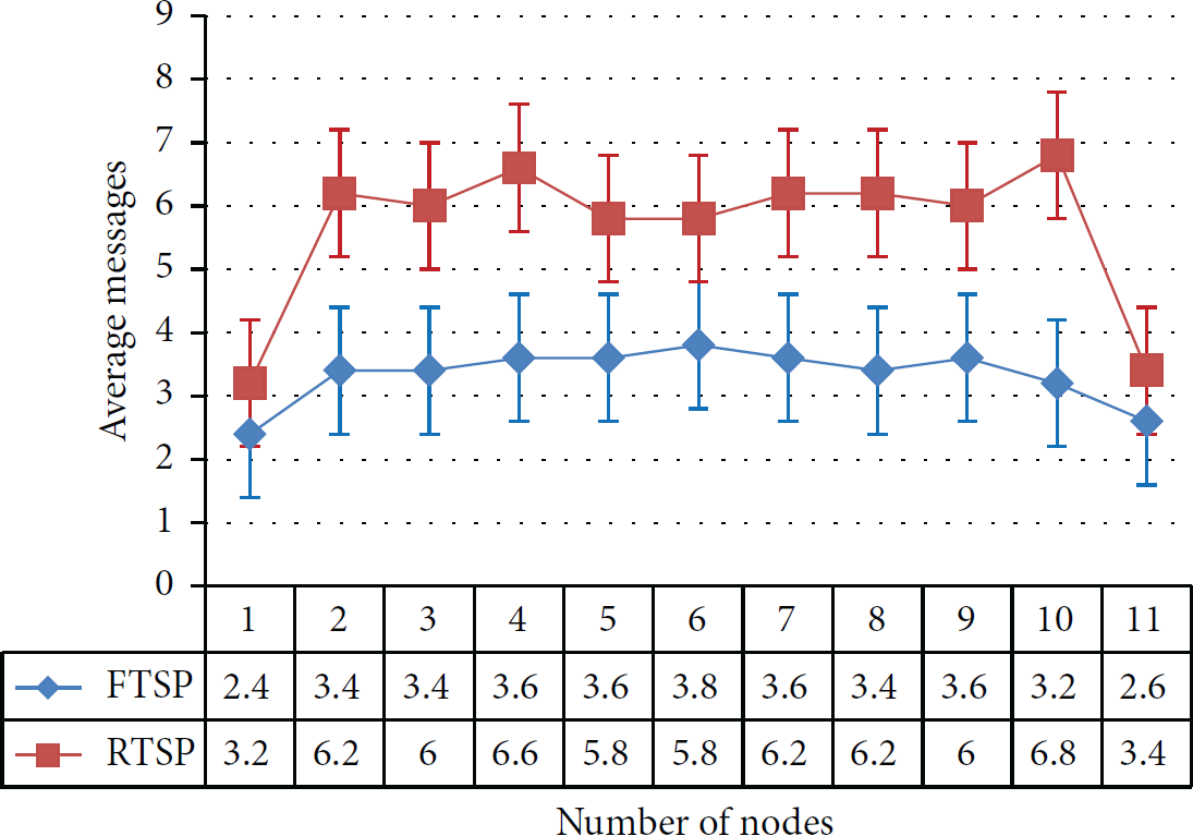
Bus topology, average number of messages per node for five experiments.

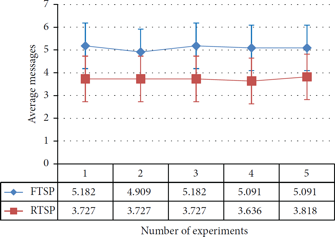
A comparison of both protocols for bus topology is shown in Figure 3. In this figure, an average of five experiments for each node is calculated. As expected, RTSP have much higher message count than FTSP. This is because of the inherent nature of RTSP that requires more number of messages per node to synchronize.

Figure 3

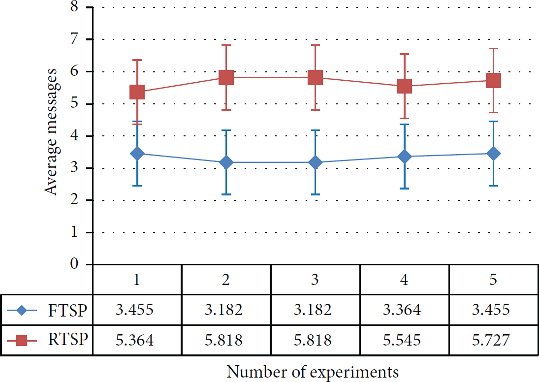
Bus topology, average number of messages for each experiment.

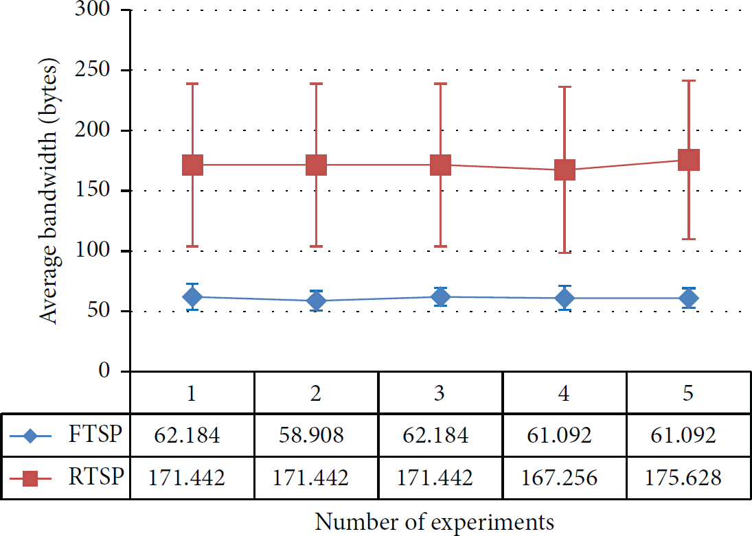
Each node's behavior varies in each experiment and is demonstrated in Figure 3. It is clearly shown that nodes' behavior is almost linear over the course of five experiments for each protocol. In addition, the variation between both protocols is almost negligible for average messages. The second metric for comparison is bandwidth. As current hardware does not provide an accurate method to measure bandwidth, we assume that their data packet size multiplied with message count equals bandwidth. Bandwidth is different from number of messages. Meanwhile, FTSP packet consists of 12 bytes and RTSP packet consists of 46 bytes.

We multiply average message and experiments average messages with FTSP and RTSP packets sizes. Accordingly, we get the average bandwidth for each node in each experiment. These results are demonstrated in Figures 4 and 5.

Figure 4

Bus topology, average bandwidth per node for five experiments.

Figure 5

Bus topology, average bandwidth for each experiment.

The difference in bandwidth between both protocols is more than four times. The main reason is due to the large packet size of RTSP and it requires more number of messages for synchronization. In RTSP, node 1 and node 11 have the lowest bandwidth consumed, because they are edge nodes and have much less interference as compared to the rest of the nodes, whereas edge nodes are directly connected with at least two nodes as compared to one node.

If we consider the general view of both metrics, FTSP clearly performs much better than RTSP. We can also deduce from these results that FTSP consumes much less energy (power) as compared to RTSP. In case of FTSP, this is due to lower bandwidth and because of transmission/reception energy conservation. Third metric used for performance evaluation is the convergence time. The average convergence time of each node over five experiments is shown in Figure 6. As we can see, convergence time for FTSP is low as well as it is consistent for most of the nodes. In case of RTSP, convergence time is zero for the initial nodes and goes up to one second for tail nodes.

Figure 6

Bus topology, average convergence time per node for five experiments.

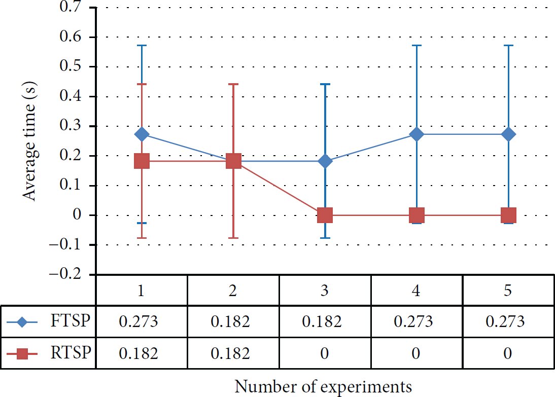
The same phenomenon happens in case of average convergence time of each experiment, as shown in Figure 7. FTSP performs better in this case as well; however, RTSP results are also acceptable. As a result, both protocols have convergence time less than 500 milliseconds.

Figure 7

Bus topology, average convergence time of each experiment.

The resulting milliseconds difference can be due to various reasons. For example, when the clock resets propagation delay may contribute to a difference of milliseconds. Hardware clock of individual nodes is also a factor. In case of convergence time, both protocols perform comparable to each other.

5.2. Grid Topology

Grid configuration makes an interesting topology, because the root node can have three different locations in the grid, as shown in Figure 8. Fifteen nodes are used for grid topology in a 5 rows × 3-column configuration. In the first configuration, root node is placed at location (1,1), that is, node 1. In this configuration, root node is directly connected with two nodes, that is, node 2 and node 6. In the second configuration, root node is placed at location (3,1), that is, node 3 and it is directly connected to nodes 2, 4, and 8. In the last configuration, root node is placed at location (3,2), that is, node 8, where it was directly connected with four nodes, that is, nodes 3, 7, 9, and 13. The most definite change would be in the number of messages, but more interesting would be the convergence time. That was our assumption before experimentation; once we started the experimentation, it became clear that the former is true, but the latter is not. Therefore, for this topology only one configuration result is shown, that is, configuration (1,1). It does not make much difference in either of the configurations for number of messages metric. To explain, let us suppose the root node is at location (3,2). The number of messages for node 7, 8, and 9 can be approximately the same, because all of the nodes are connected with four nodes from either side. The same is true for the rest of the configurations. The only difference can be the convergence time. When a node is in the center, the synchronization messages can take less amount of time. However, that may be the case for a much larger network. The speed of communication is also fast enough that makes our experiments distance independent.

Figure 8

Grid topology.

Figure 9 shows the average messages for each node for five experiments. We can see the behavior of the nodes through this figure. Nodes that are directly connected to more nodes have higher average number of messages, that is, nodes directly connected with nodes 4, 3, and 2. The most obvious observation is that FTSP performs better than RTSP in this topology for very simple reason; FTSP requires less number of messages for synchronization as compared to RTSP.

Figure 9

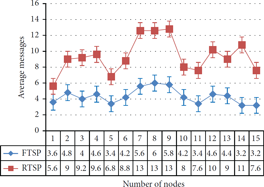
Grid topology, average number of messages per node for five experiments.

Both protocols behaved linearly in the average number of messages for each experiment, as shown in Figure 10. However, the difference in the average number of messages between protocols is almost double. RTSP performs much worst in this case. This behavior also suggests that RTSP does not perform efficiently when connected to large number of nodes. On the other hand, FTSP performs much better in this case.

Figure 10

Grid topology, average number of messages for each experiment.

Figures 11 and 12 show the average bandwidth per node for five experiments and the average bandwidth of each experiment, respectively. The bandwidth behavior is similar to the results achieved previously, because bandwidth is a function of number of messages. However, it does show how big the difference is between both protocols for bandwidth consumption. Clearly, RTSP is not very economical solution in this case. Actually, it is an expensive solution for grid topology and it remains consistent for all experiments. There is not any single case where we can conclude that RTSP is a better or comparable solution for this particular topology.

Figure 11

Grid topology, average bandwidth per node for five experiments.

Figure 12

Grid topology, average bandwidth for each experiment.

Figures 13 and 14 show the average convergence time of each node and each experiment, respectively. The average convergence time for RTSP is consistent for five experiments; that is, it remains worst. On the other hand, FTSP consistently outperforms FTSP throughout the experimentation. The average convergence time of each experiment shows interesting results. Convergence time starts high, but then it starts to reduce for both protocols. This is perhaps due to better connectivity of network for last experiments.

Figure 13

Grid topology, average convergence time per node for five experiments.

Figure 14

Grid topology, average convergence time of each experiment.

5.3. Mesh Topology

The third topology used for our experiments is mesh topology. It is fully connected mesh topology, where each node is directly connected with all the other nodes. Nodes were placed in a small area, within the antenna range of each node. Due to fully connected mesh topology, large numbers of messages are exchanged between nodes. This is the highest number of messages among four topologies for both protocols. Figure 15 shows the average messages per node for five experiments.

Figure 15

Mesh topology, average number of messages per node for five experiments.

The difference between both protocols is more than threefold. RTSP requires three times more messages than FTSP for a single synchronization cycle. On the other hand, FTSP performs significantly better. The main reason for the poor performance of both protocols, in comparison to other topologies, is that they have to deal with more number of nodes per cycle. However, in other topologies, the maximum number of nodes that are directly connected is only four nodes. Both protocols have linear behavior over the course of five experiments, as can be seen in Figure 16. On average, FTSP uses 12 and RTSP uses 36 messages/node for a single synchronization cycle. Therefore, both protocols are not very feasible for mesh topology.

Figure 16

Mesh topology, average number of messages for each experiment.

The bandwidth situation is the worst. For RTSP bandwidth consumption is always in few hundred bytes, less than one KB. However, in this case, the number reached to 1.7 KB, which is very significant for a single synchronization cycle. FTSP also has low performance, here, as compared to its performance with other topologies. Nevertheless, it is still much better than RTSP, as it can be seen in Figures 17 and 18.

Figure 17

Mesh topology, average bandwidth per node for five experiments.

Figure 18

Mesh topology, average bandwidth for each experiment.

The convergence time metric is not shown for mesh topology, because it is negligible. Almost all of the nodes have convergence time equal to zero.

5.4. Tree Topology

The physical tree topology configurations used for both protocols are shown in Figure 19. Node 1 is the root node. The rest of the configurations for both protocols are the same as described in previous sections.

Figure 19

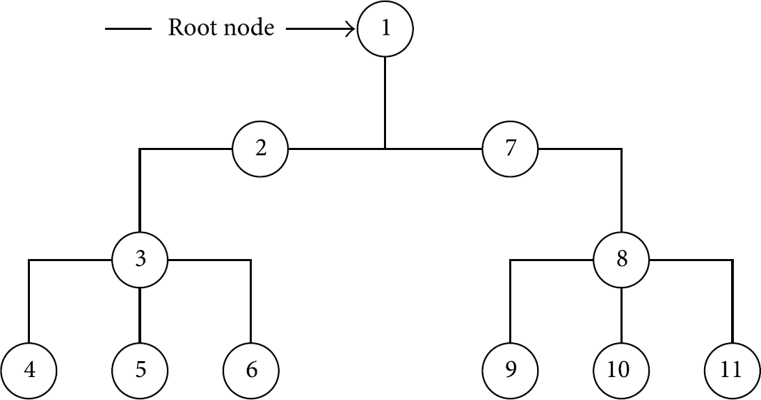
Tree topology.

Figure 20 shows a comparison between both protocols for tree topology. Average messages/node are higher for RTSP for nodes 1, 2, 3, and 8, but for the rest of the nodes they are much less than FTSP. In RTSP, high message count at some nodes is due to more connected nodes with them. Even the total message count for FTSP is high regardless of few high edges in RTSP, that is, 56 and 41, respectively. In tree topology, RTSP performs much better than FTSP for a given metric of message count.

Figure 20

Tree topology, average number of messages per node for five experiments.

The performance of both protocols for five experiments is almost linear. This means that FTSP is not the best-suited protocol for this particular topology, as shown in Figure 21.

Figure 21

Tree topology, average number of messages for each experiment.

In this topology, the bandwidth parameter makes a difference. As we have seen, RTSP utilizes less number of messages for synchronization in case of tree topology. Thus, if we rely on message count metric then RTSP is a better choice as it can be seen in Figures 22 and 23. Bandwidth consumption is high for RTSP due to the packet size and those peaks at nodes 3 and 8 are due to the connectivity with considerably large number of nodes. The difference is better demonstrated in Figure 23. Although FTSP performs slightly poorer, it is still a better protocol in terms of bandwidth consumption. RTSP is an efficient protocol in terms of synchronization for tree topology; however, it has inherent disadvantage when bandwidth is considered.

Figure 22

Tree topology, average bandwidth per node for five experiments.

Figure 23

Tree topology, average bandwidth for each experiment.

For RTSP, it is very low. The convergence time is zero for all experiments in this case. There is no delay at cluster-heads or at the root node. If there is a delay at any cluster-head at any point of time, this delay should appear in the child nodes as well. This is because RTSP uses peer-to-peer communication. On the other hand, FTSP uses broadcast for data transmission. Thus, there is no way of knowing with absolute certainty which node is synchronized from which node.

In case of the average convergence time of each node over five experiments, RTSP performs better than FTSP, as shown in Figure 24. The average convergence time for five experiments is shown in Figure 25. RTSP starts with 182 milliseconds, but, after the second experiment, it falls to zero for the rest of the experiment. Thus, RTSP performs better in the convergence time as well. Recursive Time Synchronization Protocol is designed for cluster-based topology, that is, tree topology. Therefore, it does perform better in this case. Whereas FTSP is designed for all topologies, thus, it performs better in most of the cases with the exception in tree topology.

Figure 24

Tree topology, average convergence time per node for five experiments.

Figure 25

Tree Topology, Average Convergence Time of each experiment.

6. Conclusions and Future Work

This research presented a performance evaluation of two state-of-the-art time synchronization protocols for wireless sensor networks, namely, Flooding Time Synchronization Protocol (FTSP) and Recursive Time Synchronization Protocol (RTSP). Both protocols are tested in a real-time environment using Arduino and XBee as hardware platform. The metrics used for performance evaluation are number of messages per synchronization cycle, bandwidth, and convergence time. Both FTSP and RTSP showed pros and cons. FTSP is a broadcast protocol, and it has lower accuracy at edge nodes, whereas RTSP is a peer-to-peer protocol with higher accuracy at edge nodes. FTSP performed better in bus, grid, and mesh topologies for number of messages metrics. However, RTSP has higher performance in tree topology, because this protocol was designed for cluster-based topology, that is, tree topology. On the contrary, RTSP has degraded performance for bandwidth with all four topologies, especially in mesh topology. RTSP has high bandwidth requirements. The main reason for high bandwidth requirement was the packet size of RTSP. The last metric used for performance evaluation is convergence time. The results for convergence time were inconclusive. Both protocols showed minor fluctuations in the convergence time throughout all experiments. The resolution for time measurement was in seconds, so on average none of the protocols went above one second. The main reason for convergence time inconclusiveness was the speed of communication and resolution of time measurement. According to current measurements, both protocols converged quickly. The variation in the convergence time was due to several reasons such as hardware clock variations, clock reset delays, wireless medium collisions, and several other factors. We were unable to measure the energy consumption due to hardware limitations. However, some interpretations were made from the resulting bandwidth where we considered the higher the bandwidth is the higher the energy consumption is. RTSP showed higher bandwidth consumption throughout experimentation, so it is safe to assume that it would require significant amount of energy to perform time synchronization. We observed that RTSP is an energy and bandwidth inefficient protocol as compared to FTSP in a small-scale network. RTSP is a good theoretical protocol, but not very practical in current experimentation setup. Although it solved the problem of accuracy at edge nodes, it created other problems like energy and bandwidth inefficiency. In the end, it depends on the requirement of an application; if it requires higher accuracy and has abundance of bandwidth and energy (which is not the case here) then RTSP is a better choice or if an application can tolerate slightly less accuracy then FTSP is a better choice.

In future work, we plan to compare both protocols under more flexible hardware. Bandwidth efficiency can be achieved by developing a custom sleep wake mechanism. We also plan to analyze accuracy and energy efficiency using open source tools and flexible hardware.

Footnotes

Conflict of Interests

The authors declare that there is no conflict of interests regarding the publication of this paper.

References

Hill

Horton

Kling

Krishnamurthy

The platforms enabling wireless sensor networks

Communications of the ACM 2004 47 6 41 46

10.1145/990680.990705

2-s2.0-4243132712

Bajaber

Awan

Energy efficient clustering protocol to enhance lifetime of wireless sensor network

Journal of Ambient Intelligence and Humanized Computing 2010 1 4 239 248

10.1007/s12652-010-0019-x

2-s2.0-79952443096

Johnson

Andrews

D. C.

Remote continuous physiological monitoring in the home

Journal of Telemedicine and Telecare 1996 2 2 107 113

10.1258/1357633961929871

2-s2.0-0030322246

Reina

D. G.

Toral

S. L.

Barrero

Bessis

Asimakopoulou

Modelling and assessing ad hoc networks in disaster scenarios

Journal of Ambient Intelligence and Humanized Computing 2013 4 5 571 579

10.1007/s12652-012-0113-3

2-s2.0-84884574518

Abielmona

Petriu

E. M.

Whalen

T. E.

Distributed intelligent sensor agent system for environment mapping

Journal of Ambient Intelligence and Humanized Computing 2010 1 2 95 110

10.1007/s12652-010-0010-6

2-s2.0-79952446357

Szewczyk

Osterweil

Polastre

Hamilton

Mainwaring

Estrin

Habitat monitoring with sensor networks

Communications of the ACM 2004 47 6 34 40

10.1145/990680.990704

2-s2.0-4243114087

PL-SS Distributed Surveillance Sensor Network. ONR SPAWAR Systems Center, San Diego, Calif, USA, September 2013, http://www.spawar.navy.mil/robots/undersea/dssn/dssn.html

Zeng

Xiang

Vasilakos

A. V.

Directional routing and scheduling for green vehicular delay tolerant networks

Wireless Networks 2013 19 2 161 173

10.1007/s11276-012-0457-9

2-s2.0-84878547961

Cerpa

Elson

Estrin

Girod

Hamilton

Zhao

Habitat monitoring: application driver for wireless communications technology

ACM SIGCOMM Computer Communication Review 2001 31 2, supplement 20 41

10.

Mainwaring

Culler

Polastre

Szewczyk

Anderson

Wireless sensor networks for habitat monitoring

Proceedings of the 1st ACM International Workshop on Wireless Sensor Networks and Applications (WSNA ′02)

September 2002

88 97

2-s2.0-0036986465

11.

Kim

Park

Harmon

T. C.

Real-time model parameter estimation for analyzing transport in porous media

2003

Los Angeles, Calif, USA

Center for Embedded Networked Sensing, University of California, Los Angeles

12.

Berlin

A. A.

Chase

J. G.

Yim

Maclean

B. J.

Olivier

Jacobsen

S. C.

MEMS-based control of structural dynamic instability

Journal of Intelligent Material Systems and Structures 1998 9 7 574 586

10.1177/1045389x9800900709

2-s2.0-0032274239

13.

Akyildiz

I. F.

Akan

Ö. B.

Chen

Fang

Interplanetary internet: state-of-the-art and research challenges

Computer Networks 2003 43 2 75 112

10.1016/s1389-1286(03)00345-1

2-s2.0-0042890362

14.

Burleigh

Cerf

Durst

Fall

Hooke

Scott

Weiss

The interplanetary internet: a communications infrastructure for Mars exploration

Proceedings of the 53rd International Astronautical Congress (The World Space Congress ′02)

2002

15.

Sun

Wang

Zhang

Wei

Vasilakos

A. V.

Performance of DTN protocols in space communications

Wireless Networks 2013 19 8 2029 2047

10.1007/s11276-013-0582-0

2-s2.0-84886597205

16.

Lemmerman

Delin

Hadaegh

Lou

Bhasin

Bristow

Connerton

Pasciuto

Earth science vision: platform technology challenges

Proceedings of the International Geoscience and Remote Sensing Symposium (IGARSS ′01)

July 2001

439 443

2-s2.0-0035574350

17.

De Rosa

Rus

Distributed algorithms for guiding navigation across a sensor network

Proceedings of the 9th Annual International Conference on Mobile Computing and Networking (MobiCom ′03)

September 2003

313 325

2-s2.0-1542378235

18.

Want

Hopper

Falcão

Gibbons

The ctive badge location system

ACM Transactions on Information Systems 1992 10 1 91 102

10.1145/128756.128759

2-s2.0-0026483978

19.

Werb

Lanzl

Designing a positioning system for finding things and people indoors

IEEE Spectrum 1998 35 9 71 78

10.1109/6.715187

2-s2.0-0032165502

20.

Elson

J. E.

Time synchronization in wireless sensor networks [Ph.D. thesis] 2003

Los Angeles, Calif, USA

University of California

21.

Han

Luo

Liu

Vasilakos

Algorithm design for data communications in duty-cycled wireless sensor networks: a survey

IEEE Communications Magazine 2013 51 7 107 113

10.1109/mcom.2013.6553686

2-s2.0-84880538357

22.

Cristian

Probabilistic clock synchronization

Distributed Computing 1989 3 3 146 158

10.1007/bf01784024

2-s2.0-0024946716

23.

Gusella

Zatti

Accuracy of the clock synchronization achieved by TEMPO in Berkeley UNIX 4.3BSD

IEEE Transactions on Software Engineering 1989 15 7 847 853

10.1109/32.29484

2-s2.0-0024680850

24.

Johannessen

Time synchronization in a local area network

IEEE Control Systems Magazine 2004 24 2 61 69

10.1109/mcs.2004.1275432

2-s2.0-1842680834

25.

Mills

D. L.

Internet time synchronization: the network time protocol

IEEE Transactions on Communications 1991 39 10 1482 1493

10.1109/26.103043

2-s2.0-0026242010

26.

Srikanth

T. K.

Toueg

Optimal clock synchronization

Journal of the Association for Computing Machinery 1987 34 3 626 645

10.1145/28869.28876

MR904197

2-s2.0-0023384521

27.

Yildirim

K. S.

Kantarci

Time synchronization based on slow-flooding in wireless sensor networks

IEEE Transactions on Parallel and Distributed Systems 2014 25 1 224 253

28.

Cheng

Shi

Chen

Sun

Time synchronization in WSNs: a maximum-value-based consensus approach

IEEE Transactions on Automatic Control 2014 59 3 660 675

10.1109/tac.2013.2286893

2-s2.0-84897583807

29.

Solist

Borkar

V. S.

Kumar

P. R.

A new distributed time synchronization protocol for multihop wireless networks

Proceedings of the 45th IEEE Conference on Decision and Control (CDC ′06)

December 2006

San Diego, Calif, USA

2734 2739

2-s2.0-39649121455

30.

Elson

Girod

Estrin

Fine-grained network time synchronization using reference broadcasts

SIGOPS—Operating Systems Review 2002 36 SI 147 163

31.

Maróti

Kusy

Simon

Lédeczi

Á.

The flooding time synchronization protocol

Proceedings of the 2nd International Conference on Embedded Networked Sensor Systems (SenSys ′04)

November 2004

Boulder, Colo, USA

39 49

2-s2.0-27644533289

32.

Sattar

Sheltami

T. R.

Mahmoud

A. S.

Shakshuki

E. M.

A comparative analysis of flooding time synchronization protocol and recursive time synchronization protocol

Proceedings of the 11th International Conference on Advances in Mobile Computing and Multimedia (MoMM ′13)

December 2013

Vienna, Austria

151 155

10.1145/2536853.2536945

2-s2.0-84897654297

33.

Akhlaq

Sheltami

T. R.

The recursive time synchronization protocol for wireless sensor networks

Proceedings of the IEEE Sensors Applications Symposium (SAS ′12)

February 2012

Brescia, Italy

62 67

10.1109/sas.2012.6166318

2-s2.0-84859036703

34.

Akhlaq

Sheltami

T. R.

RTSP: an accurate and energy-efficient protocol for clock synchronization in WSNs

IEEE Transactions on Instrumentation and Measurement 2013 62 3 578 589

10.1109/tim.2012.2232472

2-s2.0-84873733808

35.

Perkins

C. E.

Royer

E. M.

Ad-hoc on-demand distance vector routing

Proceedings of the 2nd IEEE Workshop on Mobile Computing Systems and Applications (WMCSA ′99)

February 1999

New Orleans, La, USA

90 100

10.1109/mcsa.1999.749281

2-s2.0-34347349933

Real-Time Performance Evaluation for Flooding and Recursive Time Synchronization Protocols over Arduino and XBee

Abstract

1. Introduction

2. Related Work

3. Hardware Setup and Limitations

4. Implementation

4.1. Flooding Time Synchronization Protocol

4.2. Recursive Time Synchronization Protocol

5. Results and Discussion

5.1. Bus Topology

5.2. Grid Topology

5.3. Mesh Topology

5.4. Tree Topology

6. Conclusions and Future Work

Footnotes

Conflict of Interests

References