
Abstract
There are many challenges in implementation of wireless sensor network systems: clustering and grouping are two of them. The grouping of sensors is computational process intended to partition the sensors of network into groups. Each group contains a number of sensors and a sensor can be an element of multiple groups. In this paper, we provided a Sensors Grouping Hierarchy Structure (GHS) to split the nodes in wireless sensor network into groups to assist the collaborative, dynamic, distributed computing and communication of the system. Our idea is to partition the nodes according to their geographical maximum covered regions such that each group contains a number of nodes and a number of leaders. To evaluate the performance of our proposed grouping structure, we have implemented a Grouped based routing and Grouped based object tracking. The proposed grouping structure shows a good performance in energy consumption and energy dissipation during data routing and it generates a little redundant data during object tracking.
1. Introduction
Like other distributed systems, WSNs are subject to a variety of unique constraints and challenges such as restricted sensing and communication ranges as well as limited battery capacity [1, 2]. These challenges affect the design of WSN [3] and bring some issues such as coverage, connectivity, network lifetime, self-managing, data aggregation, energy dissipation and energy balancing, clustering, and grouping [4, 5]. In WSNs, the node contains three main subsystems: the sensing subsystem contains one or more physical sensor devices and one or more analog-to-digital converters as well as the multiplexing mechanism to share them. The processor subsystem executes instructions pertaining to sensing, communication and self-organization [2]. The communication subsystem contains the transmitter and receiver for sending or receiving information. Due to limited range of communication, establishing the direct connection between a sensor and the base station may make the nodes transmit their messages with such a high power that their resources could be quickly depleted. Thus, the collaboration of nodes ensures the communications between distant nodes and base station. In this way, the intermediate nodes transmit messages so that a path with multiple links or hops to the base station is established [2, 6, 7]. However, the collaborative working of nodes is more critical and more complicated because of WSN natural and challenges like energy dissipation, energy balancing, location tracing, and latency. The sensors work collaboratively in many applications in our daily lives, including data collection, military applications, monitoring, and space applications [8]. For obtaining a stable collaborative work among sensors, the nodes must be able to organize themselves in structures (i.e., hierarchical structure) such that the objectives of network are achieved using the minimum cost of communication. Generally, the clustering is the most common used structure for WSNs. The clustering techniques for WSNs can be classified based on the overall network architectural and operation model and the objective of the node grouping process including the desired count and properties of the generated clusters. The research community has pursued it widely in order to achieve the network scalability objective [9]. Many of clustering algorithms [10–12] focused mainly on how to yield stable clusters with node reachability and route in environments using mobile nodes without much concern about critical design goals of WSNs such as network connectivity and coverage [9]. During the recent years, there are also many clustering algorithms designed especially for WSN, most of them mainly focused on energy dissipation, energy-balancing, and so forth.
In the literature, many protocols to reduce energy consumption have been proposed. The Low Energy Adaptive Clustering Hierarchy (LEACH) protocol [13, 14] is a cluster-based routing protocol for WSN networks that perform load balancing and ensure scalability and robustness by routing via cluster-heads and implement data fusion to reduce the amount of information overhead [15]. LEACH utilizes a randomized rotation of local cluster head to evenly distribute the energy load among the sensors in the network. After LEACH, the Power-Efficient Gathering in Sensor Information System PEGASIS [16] comes with new improvements: in PEGASIS each node communicates only with a nearby neighbor in order to exchange data, but LEACH uses single-hop routing in which each sensor node transmits information directly to the cluster-head or the sink. Regarding clustering in WSN, [17] surveys different energy efficient clustering protocols for heterogeneous wireless sensor networks and compares these protocols on various points like location awareness, clustering method, heterogeneity level, and clustering attributes. Moreover [18] presented efficient request-oriented coordinator methods for hierarchical sensor networks.
On the other hand, the traditional structures in WSNs can be categorized into data centric and location based. References [19, 20] provided two routing protocols based on data centric. In [19], Sensor Protocols for Information via Negotiation (SPIN) uses the data negotiation scheme among sensor nodes to decrease data redundancy and save energy. Direct Diffusion [20] is another data-centric routing protocol. The data generated by sensor nodes is named attribute-value pairs. When a sink node queries a certain type of information, it will send a request and the sensed data can be aggregated and then be transmitted back to the sink node. Location-based routing protocols can get the information of nodes location via GPS or any estimation algorithms based on received signal strength. Once the location information is known, the consumption of energy could be largely minimized using power control techniques [21, 22]. Based on theoretical analysis and numerical illustration under different energy and traffic models the [23] Distance-based Energy Aware Routing (DEAR) proposed an efficiently reducing and balancing of energy consumption in WSNs. During the routing process, DEAR treats a distance distribution as the first parameter and the residual energy as the secondary parameter. In the aims at maximizing the network lifetime and minimizing the energy consumption, the Two-Level Cluster base Protocol (TLCP) [24] organizes sensor nodes into clusters and forms a cluster among the cluster heads. In TLCP each cluster head transmits its data to the header of this cluster instead of transmitting directly to the far away base station and only the header can transmit data directly to the base station. The authors in [25] describe a routing protocol for wireless sensor networks based on the inclusion of routing information in the packets when minimum cost forwarding method is used. The routing table on BS is formed in the network setup phase and updated after any change in network topology reported by sensor nodes. CCM (Chain-Cluster based Mixed routing) is explained in [26]; this algorithm makes a full use of the advantages of LEACH [13] and PEGASIS [16] and provided an improved performance. CCM algorithm divides the WSN into a few chains and runs in two stages. In the first stage, sensor nodes in each chain transmit data to their own chain head node in parallel, using an improved chain routing protocol. In the second stage, all chain head nodes group as a cluster in a self-organized manner, where they transmit fused data to a voted cluster head using the cluster based routing.
As shown in Figure 1, we assumed that the interested field is covered with the minimum number of nodes such that the overlapped regions between the nodes are minimized and the nodes are expanded to cover the interested field completely. As well as, we assumed that the nodes have the same communication range indicated by the dotted circle. With such assumptions, unfortunately, if the CH nodes have the same communication range, the static clustering or dynamic clustering will not perform as efficient as peer-to-peer network.

Two different networks. The filled small circle indicates the location of node, and the dotted circle indicates the communication range of node.
This paper intended to develop and design a grouping algorithm to be used for partitioning the nodes into groups according to the maximum overlapped regions in the field. We will see the impact of this model in
The difference between clustering and grouping is simply as below:
Clustering is performed by assigning each node to a specific cluster; that is to say, each node belongs to only one cluster [8]. There is only one CH in each cluster. Grouping model is to divide the network into groups such that each node can belong to more than a group in the same time. There is more than one leader for the same group.
The rest of this paper is organized as follows. In Section 2, the grouping model and grouping algorithm are explained. The suggested network model is described in Section 3. In Section 4, we have proposed a very simple strategy for data routing based GHS. In Section 5, based on GHS, an object tracking strategy is proposed. A mechanism for avoiding data redundancy is explained in Section 6. The simulation results are shown in Section 7. Section 8 concludes this work.
2. Grouping Structure
Our main idea is to partition network's nodes into groups according to their geographical maximum covered regions in such way that each group contains a number of nodes and a number of leaders; that is, the network in Figure 2(a) contains 8 maximum covered regions (indicated by small filled circles and given a number from small filled circle 1 to small filled circle 8). That is to say, this network can be partitioned into eight groups. In Figure 2(b) the graph vertices are shown (small filled circle 1 to small filled circle 8) and each vertex represents a group of sensors; that is, the group (small filled circle 1) contains four sensors, namely, 1, 2, 3, and 4. Two groups are said to be adjacent if they contain one or more sensors in common; that is, groups ((small filled circle 1) and (small filled circle 2)) are adjacent since they have two sensors in common, namely, 3 and 4. The common sensors are called the leader of adjacent groups and they represent the edge of network graph.

12 nodes deployed randomly.
In the following, we will address the grouping problem using a simple mathematical model. Here we can present the network as a list of vectors collected by all sensors in the field. The network of n sensors is represented by a square matrix


We divide the nodes into a set of groups dynamically such that
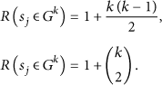
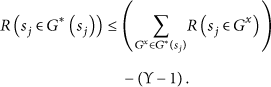
A group

A group
A group


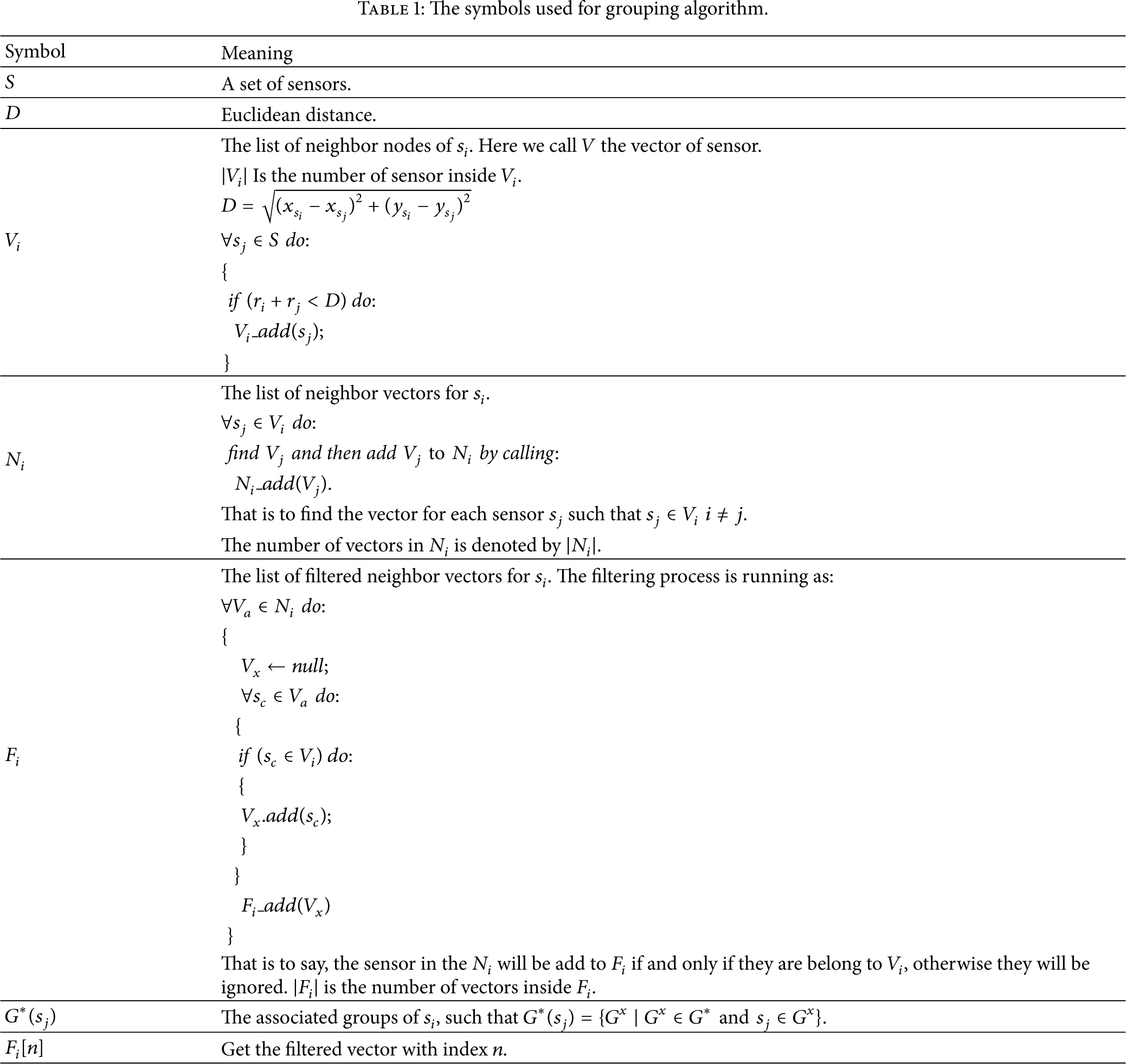
This grouping model has advantages since it makes the WSNs stress-free in many aspects such as data routing and data redundant avoiding. Below, we will provide a distributed grouping algorithm (Algorithm 1), which is executed inside the processing unit of the sensor node. However, it utilizes the information of nearby sensors to find the maximum covered regions. The symbols used for grouping algorithms are listed in Table 1.
The symbols used for grouping algorithm.
Find Input: Output: (1) (2) (3) { (4) (5) (6) (7) { (8) (9) (10) } (11) (12) { (13) (14) { (15) (16) (17) { (18) (19) (20) } (21) } (22) } (23) }
Algorithm 1 shows how the sensor node
By analyzing Algorithm 1, we can predict the resources (i.e., memory, communication bandwidth, and energy) it requires. Assume that 

3. Network Model
We model the Grouped based network using a weighted graph G, where graph vertices correspond to groups and graph edges correspond to leader sensors. By “leader sensors,” we mean the sensors that belong to more than one group. Two groups are to be adjacent if they have one sensor or more in common.
We consider a statics Graph
We assume that each sensor has a unique identifier (ID) and all sensors are aware of their geographical location and
The nodes organize themselves into groups according to Algorithm 1 such that
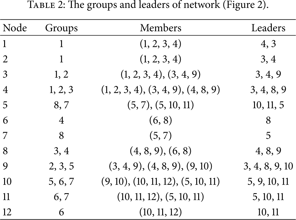
The groups and leaders of network (Figure 2).
4. Data Routing
In this section we explain a simple data routing based on grouping model. When a source node has data to send, it first started by finding the minimum distance group to the base station (Algorithm 2) and then from the selected group chooses the next hop to forward the data. The next hop can be selected according to either minimum distance to the next target node or maximum energy of target node. After maintaining the next hop (target node), the leader of the selected group will transmit the data directly to target node. After the operation of receiving data is finished, the target node finds its minimum distance group and next transmits the data recursively until the data reach the sink node. The flow chart of routing process is illustrated in Figure 4.
(1) (2) { (3) TargetGroup ← GetMinDistanceGroupFor( (4) (5) if ( (6) { (7) (8) (9) (10) } (11) else (12) { (13) (14) SinkNode.ReceiveData( (15) } (16) }
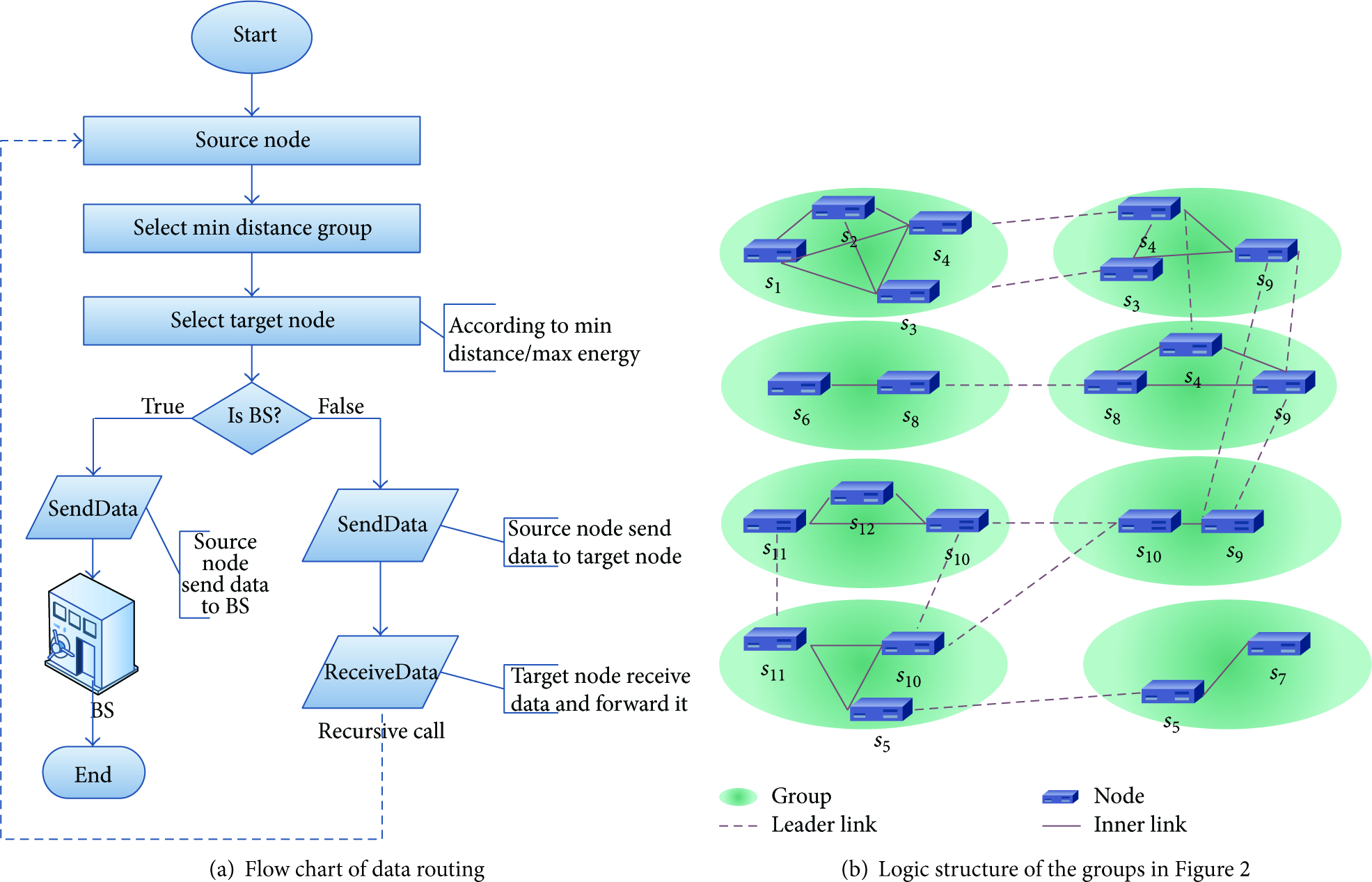
Grouped based data routing.
4.1. Energy Saving during Data Routing
The grouping model provided an efficient energy management during communication. Consider group In the same group, the none-leader to none-leader routing always leads to wastage of energy consumption. Note that the nodes in each group can communicate directly by one hop and the leaders of group acts as a gateway for the group. In the same group, the leader to leader routing sometime leads to wastage of energy consumption. In the same group, the leader to none-leader routing always leads to wastage of energy consumption.
The logical structure of grouping model for network deployed in Figure 2 is explained in Figure 4(b). When a none-leader node has data to send, it just selects one of the leaders in the group and then transmits data to the selected leader. The leader can be selected upon three main parameters:
the residual energy of leader (i.e., the leader with more energy win), the distance to source node (i.e., the nearest leader win), the current state of leader (i.e., busy or free).
5. Object Tracking and Energy Balancing
Consider a set of m mobile objects
(1) (2) (3) (4) for (int (5) { (6) (7) Root.childern.add( (8) }
5.1. Building the Notification Tree
The main objective of Notification Tree is to distribute the energy dissipation among the nodes of
For node

Notification tree.
When there is a notification message to be sent from
(1) (2) (3) (4) (5) (6) (7) (8) (9) (10) (11) (12) { (13) (14) (15) (16) (17) (18) (19) }
5.2. Building the Spanning of Subgraph
Each subgraph or component Select a vertex Assume that Select a leader node Consider Mark Repeat the steps from (2) to (4) for
6. Avoiding Data Redundancy Mechanism
An energy-efficient avoiding reporting of redundant data helps in reducing the consumed power during communications. In the following, we will mostly focus on tracking of object such that each object is allocated to one proxy node.
For

Basic storage tables.
The reporting process which intended to report the sensed data to the base station is aiming for selecting the proxy node immediately. The selection of proxy node can be determined based on the
Algorithm 5 explained our strategy for controlling the tracking mechanism of objects such that at any time there will be one node selected as a proxy node for the mobile objects.
(1) (2) (3) { (4) (5) { (6) (7) (8) (9) (10) { (11) (12) (13) (14) (15) (16) INM. (17) INM. (18) (19) (20) (21) (22) (23) (24) { (25) (26) (27) } (28) }//end if (29) (30) { (31) (32) (33) } (34) }//if (! isInMyNMT(mobj)) (35) }//end if (36) (37) { (38) (39) (40) { (41) (42) (43) (44) (45) } (46) }
In line number 26, the function
7. Results and Discussion
In this work, we assumed that the radio channel is symmetric such that the energy required to transmit a message of k bits from node x to node y is the same as energy required to transmit the same size message from node y to node x for a given signal to noise ratio (SNR). We assume a simple model called (First Order Radio Model). This model discussed in [13–16]. For this model, the energy dissipation to run the radio (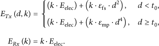
For performance evaluation, we developed a software using c# (Visual Studio 2012). We will use three different coverage schemes as shown in Figure 7.

The network topologies used to simulate the performance of GHS. The arrow indicated the position of base station (sink node). The green progress bar indicates the residual energy. Here all nodes are full charged 0.5 Joule.
7.1. Grid Based Coverage
For grid based coverage schemes, we have selected two algorithms provided in [27], Grid Square Coverage version (1) and Grid Square Coverage version (2). Grid Square Coverage (1) algorithms have 78% coverage efficiency while Grid Square Coverage (2) has 73%.
7.1.1. Grid Coverage Version (1)
Table 3 shows the parameters we used to evaluate the performance of GHS in grid coverage version (1). The sensors deployed are as shown in Figure 7(a).
Simulation parameters.

The evaluation results for using GHS on grid coverage version (1) are shown in Figures 8 and 9. In Figure 8, the residual energy (in joule) is explained after each node of 182 nodes sent five message of size 1024 bits (five rounds). It indicates that the closed nodes to base station will die out first due to network load. As the communication range of far node is limited, the close nodes to base station will act as routers for forwarding packets that transmitted from far nodes. In addition, Figure 9 explained the dead nodes after 100, 200, and 300 rounds.

The residual energy of nodes after five rounds. We assume that the battery of each node is 0.5 J. Network topology is grid version (1).

The dead nodes (brown) after 100, 200, and 300 rounds using grid coverage 1 topology. The initial energy is 0.5 J/node with 50 nJ/bit dissipation to run the radio (
In this coverage scheme, the number of nodes in each group is 4, which means more channels for leaders to forward data. The average number of nodes in each path (the number of hops) is 4.5 when radius is 25 m. The min distance for each group is 35 m and the max distance is 49 m, that is to say, for any message (1024 bits) to be sent from node A to node B it either consumes 76288 nJ or 63744 nJ.
7.1.2. Grid Coverage Version (2)
Table 4 shows the parameters we used to evaluate the performance of GHS on grid coverage version (2). The network topology is shown in Figure 7(b).
Simulation parameters.

In Figure 10, the residual energy (in joule) is explained after each node of 181 nodes sent five messages of size 1024 bits (five rounds). Figure 11 explained the die out node after 100, 200, and 300 rounds. In this coverage scheme, the number of nodes in each group is 2, which means there are two channels for leaders to forward data. The average number of nodes in each path (the number of hops) is 6.29 when radius is 25 m. The min distance for each group is 33 m and the max distance is 36 m, that is to say, for any message (1024 bits) to be sent from node A to node B it either consumes 62996.48 nJ or 64020.48 nJ.

The residual energy of nodes after five rounds. We assume that the battery of each node is 0.5 J. Network topology is grid version (2).

The dead nodes (brown) after 100, 200, and 300 rounds using grid coverage 2 topology. The initial energy is 0.5 J/node with 50 nJ/bit dissipation to run the radio (
7.2. Zigzag Based Coverage
In zigzag coverage scheme, the interest area divided into multiple zigzag patterns with multiple corners and lines segments, each node is deployed in a corner of zigzag pattern. Zigzag Pattern Scheme Deployment Algorithm expresses a very high coverage efficiency of 91%, and it expands and covers the whole interest area with minimum number of nodes, while it generates a very small coverage redundancy [28]. Table 5 shows the parameters we used to evaluate the performance of GHS on zigzag coverage sachem [16]. The network topology for zigzag is shown in Figure 5(c) (Table 5).
Simulation parameters.

In Figure 12, the residual energy (in joule) is explained after each node of 138 nodes sent five messages of size 1024 bits (five rounds). It indicates that the closed nodes to base station will die out first due to network load. Due to limited communications range of far node, the close nodes to base station will act as routers for forwarding packets that transmitted from far nodes. Figure 13 explained the amount of energy consumed by each node for the same number of rounds. In addition, Figure 14 explained the die out node after 100, 200, and 300 rounds. In this coverage scheme, the number of nodes in each group is 3, which means there are three channels for leaders to forward data. The average number of nodes in each path (the number of hops) is 4.6 when radius is 25 m. The min distance for each group is 43 m and the max distance is 44 m, that is to say, for any message (1024 bits) to be sent from node A to node B it either consumes 70605.856 nJ or 71069.7216 nJ. In Figure 15, the GHS executed 1000 rounds for the three coverage schemes depicted in Figure 7. Table 6 shows the comparisons between GHS and other well-known structures over different topologies and different initial energy.
Comparison between GHS and other well-known structures over different topologies and different initial energy.
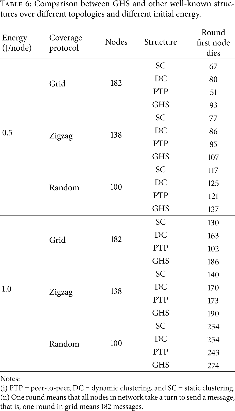
Notes:
(i) PTP = peer-to-peer, DC = dynamic clustering, and SC = static clustering.
(ii) One round means that all nodes in network take a turn to send a message, that is, one round in grid means 182 messages.
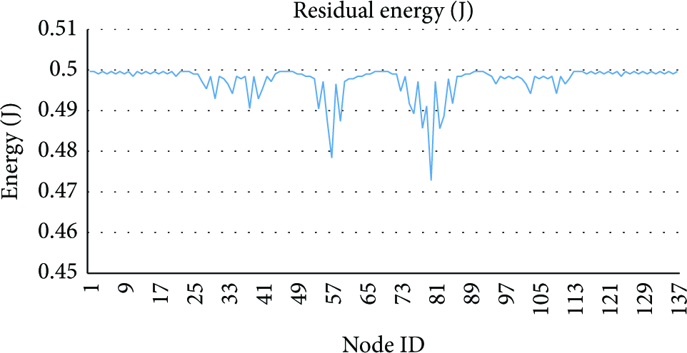
The residual energy of nodes after five rounds. We assume that the battery of each node is 0.5 J. Network topology is zigzag.

The consumed energy of nodes after five rounds. We assume that the battery of each node is 0.5 J. Network topology is zigzag.

The dead nodes (brown) after 100, 200, and 300 rounds using zigzag topology. The initial energy is 0.5 J/node with 50 nJ/bit dissipation to run the radio (
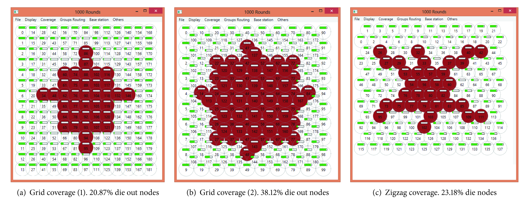
The dead nodes (brown) of three coverage schemes after 1000 rounds of GHS, and the battery of each sensor is 0.5 J. In each round each sensor sends a packet of 1024 bits. The energy dissipation to run the radio (
8. Conclusion and Further Works
This paper intended to develop a Sensors Grouping Hierarchy Structure (GHS) for partitioning the nodes into groups according to the maximum overlapped regions in the field. A group of sensors contain multiple number of nodes and a multiple number of leaders, and each node can belong to more than one group. We assumed that the interest field is covered with the minimum number of nodes such that the overlapped between the nodes is minimized and the nodes are expanded to cover the interested field completely. This structure enhances the collaborative, dynamic, distributive computing and communication of the system, and it maximizes the lifespan of nodes by minimizing energy consumption, balancing energy, and generating a little redundant data.
For further research, we plan to extend our structure by studying the influence of nodes quick movement in the field. And we will study the object tracking intensively using this structure. The researchers are very welcomed to develop energy efficient data routing algorithms and objects tracking algorithms using GHS.
Footnotes
Conflict of Interests
The authors declare that there is no conflict of interests regarding the publication of this paper.
Acknowledgments
The authors would like to thank the anonymous reviewers for the helpful comments and suggestions. The National Natural Science Foundation of China (nos. 61472382, 61272472, and 61232018) and the National Science Technology Major Project (no. 2012ZX10004301-609) support this paper.