Sage Journals: Discover world-class research

Abstract

In-network data aggregation is a widely used method for collecting data efficiently in wireless sensor networks (WSNs). The authors focus on how to achieve high aggregation efficiency and prolonging networks’ lifetime. Firstly, this paper proposes an adaptive spanning tree algorithm (AST), which can adaptively build and adjust an aggregation spanning tree. Owing to the strategies of random waiting and alternative father nodes, AST can achieve a relatively balanced spanning tree and flexible tree adjustment. Then a redundant aggregation scheme (RAG) is illustrated. In RAG, interior nodes help to forward data for their sibling nodes and thus provide reliable data transmission for WSN. Finally, the simulations demonstrate that (1) AST can prolong the lifetime and (2) RAG makes a better trade-off between storage and aggregation ratio, comparing to other aggregation schemes.

1. Introduction

Wireless sensor networks, as a promising technology, have been attracting more and more interest from the research community for a broad range of applications. Typical WSN applications involve lots of distribute-deployed sensors and one or more base stations (each of which is called the sink). Each sensor can sense, collect, and transmit information to the sink periodically or in events-driven style.

However, WSN is challenged by its limited capacity of communication and computation, limited power supply, and high vulnerability to failures. Among all the challenges, power supply is a big issue, especially under the wretched and inaccessible network environments. Thus, it is critical to save energy and collect data efficiently and correctly. On the ground, it has attracted much attention to design communication protocols for topology management and in-network aggregation [1–3].

The design of in-network aggregation [4–8] is a well-studied energy efficient data collection method and has been applied in other cases [9]. This owes to the following two aspects. First, if sensors send their original readings directly to the sink without local process, it will usually occupy excessive bandwidth and consume too much energy because of the redundancy in these original readings. Second, what the applications need usually are not the original sensor readings but the processed data. These two aspects make in-network aggregation possible and necessary. The basic idea of in-network aggregation is that redundant and irrelevant data are discarded and the relevant data are fused into an aggregation result at interior nodes along the transmission paths. Thus, data size and traffic are reduced, which will save considerable energy.

2. Related Work

In WSNs, data aggregation is closely related to the network structure, such as tree-based [10–12], cluster-based, and hybrid structures [8]. In particular, the tree-based structure has attracted many researchers and different tree-based aggregation algorithms have been proposed to both reduce energy consumption and maximize the lifetime [13–15].

Paper [10] proposes an aggregation tree construction/reorganization algorithm that minimizes such desired metrics as energy consumption. By calculating and sending a small set of intuitive statistics, a father node may be substituted by one of its brother nodes based on attachment cost.

Both [11, 12] propose the so-called life-time preserving tree (LPT). While building the aggregation tree, LPT chooses nodes with higher residual energy as aggregating fathers. In E-span tree (energy-aware spanning tree) [12] algorithm, each node uses two measurement to choose its father. The principle one is the depth nodes located in the spanning tree, and another is the residual energy.

Different from E-span, EE-span (energy efficient spanning tree) algorithm in [13] uses nodes’ residual energy as the main parameter and the distance as the complementary. That is, the selected father node has the most energy and the distance is reasonable. Recall that the transmission power is directly related to the distance. So, EE-span in fact takes the average path's energy as a new parameter when choosing father nodes.

AEE-span, an automata-based energy efficient spanning tree proposed in [14], uses learning automata to dynamically compute the probability that a node can be selected as a father node according to environment information such as distance or residual energy. Then, the node with the biggest probability is selected as a father node.

Whatever measurements are used, all strategies above have two things in common. Firstly, a node cannot determine its father until it collects all the environment information from all its neighbors and selects the one who fits the measurement best. This may lead to a big problem. The so-called best node is prone to be selected by lots of nodes in the same area, which makes this node a kind of bottleneck since it is responsible for data aggregation and transmission for all its huge children. Secondly, they will rebuild the aggregation tree periodically, which is energy-consuming and time-wasting [15].

Another important issue is how to aggregate sensors’ data via the constructed tree. One simple but popular aggregation operation is TAG illustrated in [2]. Firstly each leaf node in the tree reports data to its parent; then interior nodes aggregate data of their children and report the aggregated data to their parent. Obviously, TAG has only one single path for a node to transmit data for itself and its children if having some. Thus, if an interior node fails to communicate with its parent, all the data collected by it and its children cannot be sent to the root.

To sum up, while using tree-based structure to aggregation data, both the tree construction and updating and the aggregation scheme need improvement to achieve a robust and efficient data collection in WSNs. This is also the scope/aim of our paper. The main contribution of this paper lies in the following three aspects. (1) We let each node set a random waiting time to determine its father node via a specific criterion. According to this strategy, we can avoid that a favorable node has lots of child nodes and then becomes a bottleneck. (2) By the strategy of setting up alternative father nodes, any father node can be replaced by more occupied node asynchronously. Thus, no tree rebuilt is needed. Our tree construction and update strategies are called AST hereafter. (3) Enlightened by the multipath transmission idea of RING in [16], we propose RAG, a redundant aggregation scheme, to achieve flexible and efficient data aggregation and transmission in the tree structured network.

3. Network Models and Definitions

3.1. Network Models

In this paper, we assume that certain amounts of sensor nodes are uniformly deployed in an $m \times m$ square area. Sensor nodes have the following characteristics: (1) in the network, all nodes are stationary after being deployed; (2) all nodes are of different amount of initial power and the sink has infinite power; (3) the sink can be deployed anywhere in the monitoring area; (4) all nodes have the same sensor radius, denoted as R.

We adopt query-style aggregation strategy like that in [2]. The aggregation process includes two important phases, the query distribution phase and the data collection phase. During the query distribution phase, the sink generates and broadcasts tree construction message (msg_GTD, as illustrated in Section 3.2) in which the query is included. Then, this msg_GTD will flood through the network to construct the aggregation tree. In order to focus on aggregation operation, we simplify the model and assume that loose synchronized time and assigned aggregation interval are used as in [16], and these ensure each father node receives all children's aggregation results and its original sensor readings. During data collection phase, each node's aggregation interval is the same and is divided into 3 subintervals which will be illustrated in Section 5.

The collection phase starts from leaf nodes and the aggregation is carried out at each interior node along the aggregation tree interval by interval. Finally, an aggregation result is generated at the sink.

3.2. Related Definitions and Abbreviations

As shown in Table 1, we define a series of entities as functions, messages, or data structures necessary for accomplishing our algorithms. Prefixes data_, msg_, and func_ in entity's name are used to illustrate that the entity is a data structure or a message or a function, respectively. Each sensor node maintains not only its attributions but also the information about its parent or alternative parents. Nodes use the data structure entities to maintain all of its necessary information and use the function entities to process the data or maintain the tree structure and use the message entities to transfer messages in network.

Table 1

Entities needed in this paper.

Entity name	Remark
data_FS	To store node's alternative father nodes

data_AR	To store node's aggregation results by itself

data_ARc	To store node's all aggregation results received from children

data_ARs	To store node's all aggregation results received from siblings

msg_GTD	A query message which may initiate a tree construction process

msg_DATA	A message contains the aggregation data that is transferred in network

func_SG	A function that fuses sensor readings into local aggregation results

func_SF	A function that fuses sensor siblings’ and local aggregation results together

func_SFA	A function that selects and sets a new father node from its data_FS

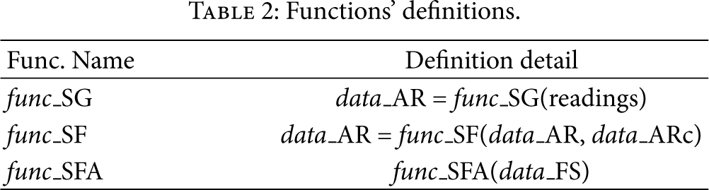
A node has such attributions as ID, LEVEL, fID, fLEVEL, pos_X, pos_Y, fDIS, and so forth. ID and fID indicate the node and its father's ID, respectively. LEVEL and fLEVEL indicate in which level the node and its father are located in the spanning tree. pos_X and pos_Y are the positions of this node. fDIS indicates the distance between this node and its father. Now, let us give the detailed structure of the message, msg_GTD and msg_DATA, which is very important in the procedure of tree construction. msg_GTD is generated by a node and contains at least six important attributions of the node, that is, ID, LEVEL, fID, fLLEVEL, pos_X, and pos_Y. The detailed definitions of all the functions are shown in Table 2.

Table 2

Functions’ definitions.

Func. Name	Definition detail
func_SG	data_AR = func_SG(readings)
func_SF	data_AR = func_SF(data_AR, data_ARc)
func_SFA	func_SFA(data_FS)

4. Adaptive Spanning Tree (AST)

4.1. Tree Construction

To build an adaptive spanning tree, we also let the sink initiate the construction process and flood the msg_GTD among the network. Different from others, every node uses asynchronous random wait mechanism to determine the ultimate father node. Also, we will collect all the alternative father nodes and store them in the set of alternative father nodes (data_FS) for every node. Algorithm 1 shows the detail of AST.

Algorithm 1: Algorithm of building up the spanning tree by AST.

(1) if(node.fID $= =$ 0) {/^*node hears msg_GTD for the first time^*/

(2) node.LEVEL = msg_GTD.LEVEL + 1;

(3) node.fID = msg_GTD.ID /^*setting node msg_GTD.ID as its temporary father^*/

(4) node.fDIS = cal_distance(node, msg_GTD.ID) /^*calculating and storing the distance to its father^*/

(5) data_FS = data_FS ∪ {msg_GTD.ID} /^*setting the msg_GTD.ID as its alternative fater^*/

(6) setTimer(random()); /^*setting random waiting time^*/ }

(7) while(not time out) { /^*if random time is not up^*/

(8) if(node.LEVEL $= =$ msg_GTD.LEVEL + 1) {

(9) data_FS = data_FS ∪ {msg_GTD.ID} /^*setting the msg_GTD.ID as its alternative fater^*/

(10) Dis1 = cal_distance(node, msg_GTD.ID)

(11) if(node.fDIS < Dis1 && Dis1 < $R / 2$ ) /^*a new better choice is found, do exchange^*/

(12) {node.fDIS = Dis1; node.fID = msg_GTD.ID; } }

(13) else if(msg_GTD.LEVEL $= =$ node.LEVEL)

(14) {data_FS = data_FS ∪ {msg_GTD.ID $}}$ /^*setting the msg_GTD.ID as its alternative fater^*/

(15) When time out, node updates msg_GTD with its own information then forwards this msg_GTD

Here goes the exploration of the asynchronous random wait mechanism. When a node, saying $N_{i}$ , hears the msg_GTD for the first time, it selects the sender of this msg_GTD as its undetermined father and sets its LEVEL according to the level information in the msg_GTD. Rather than rebroadcasting the msg_GTD immediately, $N_{i}$ will set a random time interval to wait. During this time interval, $N_{i}$ will collect all msg_GTD messages from its neighbors if any and select a more favorable one. Specifically speaking, if $N_{i}$ receives an msg_GTD from another node (we call this node $N_{i}$ 's new possible father), it will replace the current undetermined father by the new possible father only when it satisfies the following two conditions: (1) the distance to the new possible father is shorter than that to the undetermined father; (2) the distance to the new possible father is less than half the sensor radius. When the random waiting time is out, $N_{i}$ sets the current undetermined father as its father and updates and forwards the msg_GTD. In this process, $N_{i}$ will update its alternative father nodes set, that is, data_FS, whenever it receives an msg_GTD which will be illustrated more specifically later.

Given the connectivity diagram in Figure 1, we illustrate the proposed AST algorithm and compare the differences between different algorithms. There are $N_{1}$ to $N_{8}$ , and their residual energy is 10 J, 8 J, 6 J, 3 J, 4 J, 7 J, 9 J, and 8 J. Suppose $N_{1}$ broadcasts msg_GTD and $N_{6}$ is going to determine its father node. Now, let us explore how to construct spanning trees by different algorithms.

Figure 1

Connectivity diagram.

The TAG constructs the simplest tree (as in Figure 2(a)). When $N_{2}$ , $N_{3}$ , $N_{4}$ , and $N_{5}$ , neighbors of $N_{1}$ , receive this msg_GTD and select $N_{1}$ as their father, then $N_{6}$ receives an msg_GTD from $N_{3}$ . So, $N_{6}$ chooses $N_{3}$ as its father immediately. E-span tends to find a node that is nearer to sink as father node and EE-span tends to find a node that is of the most average path's energy as father. E-span and EE-span continuously compare the nodes from which they receive msg_GTD to decide the most qualified father during the whole tree building period. So, $N_{6}$ compares $N_{2}$ , $N_{3}$ , and $N_{7}$ to decide which node is its father according to the respective criterion. The final spanning tree of E-span and EE-span can be seen in Figures 2(b) and 2(c). Using AST, $N_{6}$ firstly receives an msg_GTD from $N_{2}$ and $N_{6}$ waits a random time interval. During this interval, $N_{6}$ receives an msg_GTD from $N_{3}$ , because $D_{26} > D_{36}$ and $D_{36} < R / 2$ (here, $D_{i j}$ refers to the distance between $N_{i}$ and $N_{j}$ . R is the sensing radius of each node). $N_{3}$ is selected as father and the random waiting of $N_{6}$ is over. Figure 2(d) shows the spanning tree constructed by AST.

Figure 2

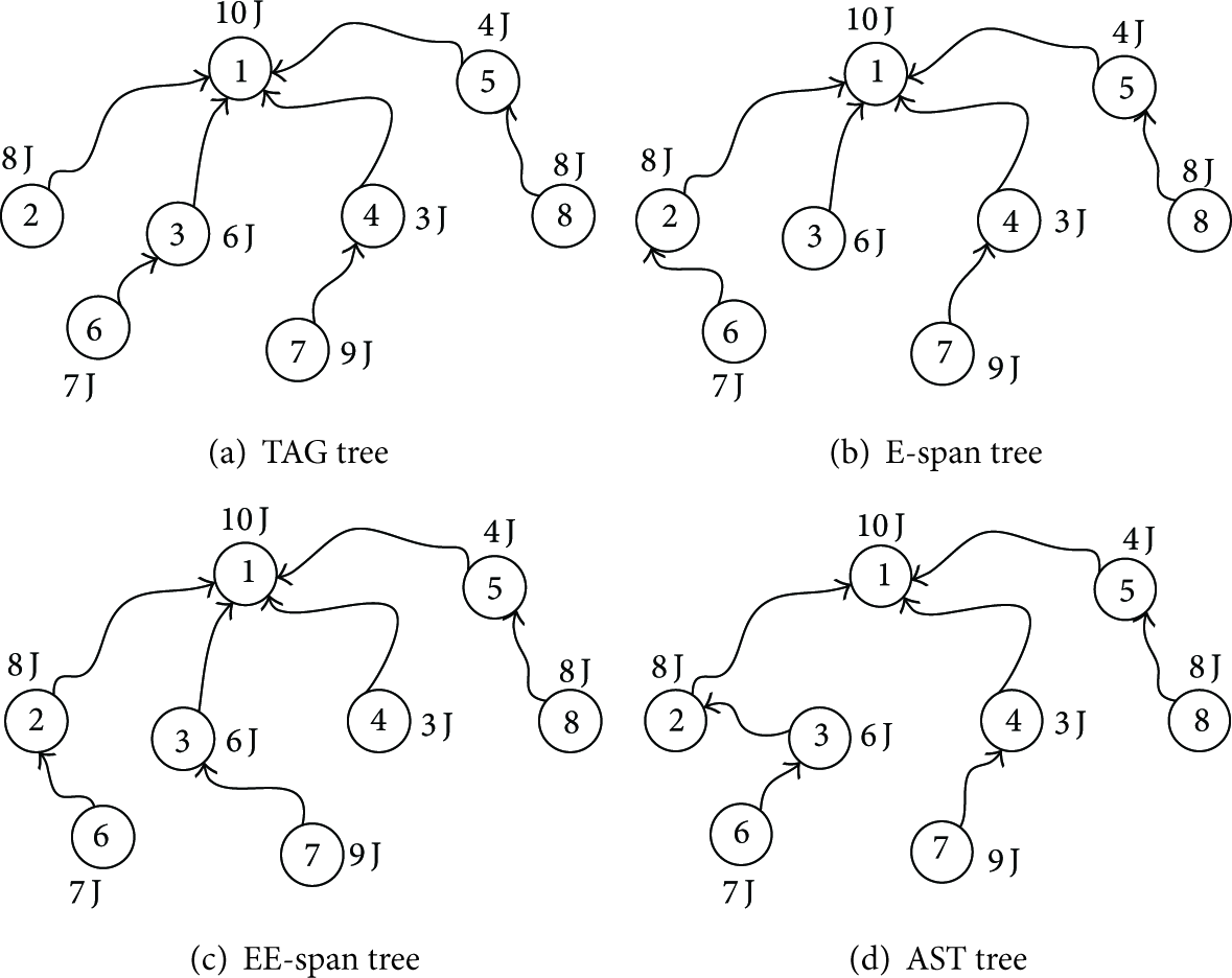
Aggregation trees of different algorithms.

4.2. Tree Maintenance

Another critical feather of AST is the local adjustment strategy that is carried out when finding a failure father. Recall that each node, say $N_{i}$ , sets up its alternative father nodes and stores them in its data_FS during the tree building period. During the random waiting time, if $N_{i}$ hears an msg_GTD from the nodes with the same level as $N_{i}$ 's father or $N_{i}$ itself, $N_{i}$ will add the msg_GTD's sender to its data_FS. We constrain $N_{i}$ 's alternative father nodes level to avoid circles in the tree. Moreover, since these nodes are relatively closer to the sink node than those in the child level, the times for transmitting data of $N_{i}$ will be smaller if they are set as a father node. This data_FS will be maintained during the whole lifecycle of WSN whenever the local adjustment strategy is used to update the spanning tree.

Take Figure 3(a) as an example. $N_{2}$ , $N_{3}$ , and $N_{6}$ are in the same level, while $N_{5}$ and $N_{7}$ are from $N_{2}$ 's father level, and $N_{7}$ is $N_{2}$ 's father. $N_{2}$ adds $N_{3}$ , $N_{5}$ , and $N_{6}$ to its data_FS when constructing the AST. That is, $N_{2}$ 's alternative father nodes include $N_{5}$ , $N_{6}$ , and $N_{3}$ .

Figure 3

Alternative father nodes illustration.

In WSN, message sending behavior of a node is a kind of its heartbeat which can be heard passively by its neighbors. Thus, during the lifecycle of the network, AST uses this passive heartbeat detecting strategy to update nodes’ data_FS and detect father node's status. For a node $N_{i}$ , if it cannot hear a passive heartbeat from its alternative father, say $N_{j}$ , for a period of time such as l successive aggregation intervals, $N_{i}$ may think $N_{j}$ is a failure and remove it from the alternative father set data_FS. Similarly, if $N_{i}$ finds that its father node is a failure, it will be replaced by selecting a favorable alternative node from its data_FS (using function func_SFA) according to the residual energy.

Now, we will use an example to illustrate this strategy. As in Figure 3(a), if $N_{2}$ can hear the passive heartbeat from $N_{7}$ during an aggregation interval, $N_{2}$ records that, at this aggregation interval, $N_{7}$ is in a normal status; else, $N_{2}$ records that $N_{7}$ is abnormal. $N_{2}$ will record the latest n statues of each alternative father node. If spare father node's latest n statuses are all abnormal, they indicate that this alternative father node is broken. It is deleted from the data_FS. If $N_{7}$ , $N_{2}$ 's current father node, is thought to be a failure, apart from deleting it from data_FS, $N_{2}$ will also select a new father from its data_FS based on the residual energy. That is, the node in $N_{2}$ 's data_FS with the biggest residual energy will be set as the new father of $N_{2}$ . We assume that the residual energy of $N_{3}$ , $N_{6}$ , and $N_{5}$ is 5 J, 6 J, and 10 J, respectively. Then, $N_{5}$ will be selected to be the new father. We can see that even if $N_{7}$ dies its child node $N_{6}$ and $N_{2}$ can locally find a replacement, the connectivity of network is maintained (Figure 3(b)). This strategy is asynchronous and distributed for sensor nodes. Unlike other current spanning tree construction algorithms, periodical reconstruction of aggregation tree is not needed in AST. So, it is more flexible and energy-saving.

5. Redundant Aggregation Scheme

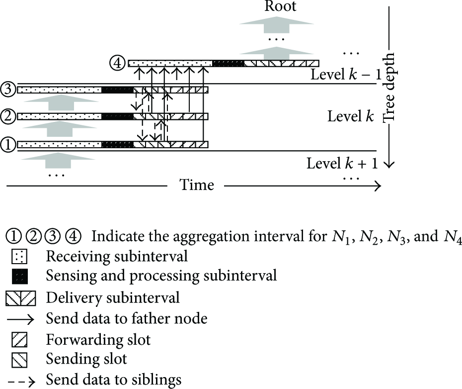
In this section, we propose redundant aggregation scheme for tree structure. This scheme changes the single-path transmission of the traditional tree aggregation scheme and allows the nodes to transmit data for their siblings. In our aggregation scheme, when a nondestination node receives a message, it firstly checks if this message is from its siblings. If so, it will store and forward this message to its father node. This forms our redundant aggregation scheme RAG. In RAG, nodes’ tasks in their data aggregation interval are illustrated as follows.

(1) Receiving Subinterval. In this subinterval, interior nodes have two tasks. Firstly, nodes receive the uploaded aggregation results from their children. Secondly, interior nodes detect and delete duplicated data to build the local results. For the leaf nodes, they do not have this subinterval.

(2) Sensing and Processing Subinterval. In this subinterval, interior nodes read their sensing data and aggregate it with the local results built in receiving subinterval and thus make the aggregation results ready for sending. For the leaf nodes, there is no aggregation process during this subinterval.

(3) Delivery Subinterval. This interval is divided into sending slot and forwarding slot. In the sending slot, nodes send their own aggregation results to their father nodes and receive the aggregation results from siblings, if they have, and store them for forwarding. Then, they forward the data for their siblings, if they have, in forwarding slot. The pseudocode of redundant aggregation is illustrated in Algorithm 2.

Algorithm 2: Redundant aggregation.

/^*receiving sub-intervals start^*/

(1) data_ARc = receive(); /^*nodes receive data messages from its child nodes^*/

(2) data_ARc = deleteDuplicate(data_ARc); /^*delete duplicated data^*/

/^*sensing and processing sub-intervals start^*/

(3) data_AR = func_SG(readings); /^*generate original sensor reading^*/

(4) data_AR = func_SF(data_AR, data_ARc); /^*sending sub-intervals start^*/

/^*sending slot^*/

(5) Send(data_AR); /^*send Data to father node^*/

(6) data_ARs = receive(); /^*receive data from siblings^*/

/^*forwarding slot^*/

(7) Send(data_ARs); /^*forward the aggregation results from its siblings to its father node^*/

Now, we use an example to demonstrate the detail of RAG as shown in Figures 4 and 5. Before we explore RAG, we firstly illustrate the problems that the traditional tree aggregation schemes face. As can be seen from Figure 4(a), $N_{1}$ , $N_{2}$ , and $N_{3}$ are $N_{4}$ 's children. $N_{1}$ 's message is heard by $N_{2}$ and $N_{3}$ , but $N_{2}$ and $N_{3}$ discard it because they are not $N_{4}$ 's father node. Thus, there is only one single link between $N_{1}$ and $N_{4}$ . If this unique link is broken, $N_{1}$ 's message cannot be transmitted to $N_{4}$ , which leads to the subtree leading by $N_{1}$ isolated from the network. Luckily, the messages deleted by brothers can be leveraged to form our RAG. When $N_{2}$ and $N_{3}$ receive the message whose destination is $N_{4}$ , their father node, they do not delete this message but store it. Then, they forward it to $N_{4}$ . So, in Figure 4(b), there are 3 different links that connect $N_{1}$ with $N_{4}$ . Thus, even if the direct link between $N_{1}$ and $N_{4}$ is broken, there are two extra paths. Figure 5 illustrates RAG in more detail by time slot. To avoid collision, father allocates time slot for each child during sending slot and forwarding slot.

Figure 4

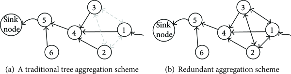
Illustration of redundant aggregation.

Figure 5

Redundant aggregation on each time slot.

6. Simulation

6.1. Simulation Setup

Here, we evaluate the performances of AST and RAG separately. We compare AST with another three popular tree structures, TAG, E-span, and EE-span, by simulation. For the aggregation schemes, we compare RAG with TAG and RING.

In all our simulations, we uniformly deploy a number of sensor nodes whose sensing radius is 4 m on a 25 m × 25 m square area and a sink node in the center of the simulation area. We vary the number of nodes from 100 to 500, with the increment step of 50. When setting up the simulation environment, we initialize every node with energy randomly selected from 800 J to 1000 J and also suppose the sink has infinite energy. We suppose that the energy consumption for nodes to process data is negligible, and the energy consumption for message receiving and transmitting satisfies formulas (1) and (2) in [13] with $C_{1}$ and $C_{2}$ set to 1 and 5, respectively, in our simulations.

To make the analysis more reasonable, we conduct 500 independent simulations to get an average result in all our analysis.

6.2. Simulation-Based Analysis of AST

We compare the network lifetime, average levels, and number of alive nodes among AST, E-span, EE-span, and TAG. As can be seen from previous illustration, in the tree-based aggregation WSN, the system runs round by round. A round is one complete cycle for collecting sensor readings, aggregating data, and transmitting the aggregated data to sink. Namely, a round ends when the sink receives aggregation results from all its alive child nodes. We also define that the network is failure if 5% nodes fall failure as in [13]. Thus, the number of rounds before the network is a failure indicates the network lifetime.

We define the level of node which means the depth a node locates in the spanning tree. The level of node indicates the number of nodes along the path between the sink and the node itself. We further define average level as the mean of all levels of all nodes in the network. It is obvious that a less average level means that the average degree [17] of the spanning tree is bigger and that interior nodes averagely have more children.

In Figure 6(a), the average levels of AST and EE-span are crossed, and their levels are higher than the levels of TAG and E-span. So, the average degrees of AST and EE-span are smaller, which indicates that they averagely have less child nodes per father node than TAG and E-span. Any interior node with less child nodes has less communication requirement per round. Recall that communication is the major factor of energy consumption. Thus, the nodes in AST and EE-span are more likely to live longer than TAG or E-span; hence, the entire network lifetime of them is bigger, which coincides with Figure 7.

Figure 6

Performance of AST.

Figure 7

Performance of RAG.

Figure 6(b) shows the trend of the network lifetime. The lifetime of AST can be prolonged when adding nodes to the network, while E-span and EE-span change a little. As illustrated in Sections 1 and 4, unlike AST which only uses physical distance among nodes as the most important issue, EE-span and E-span take the residual energy as an important issue while constructing the spanning tree. Thus, EE-span and E-span may select the most powerful nodes as a father node. But the physical distance between father and its child node may be large which hence consume more energy during the collection phase. That is to say, AST relies more on the physical distance among nodes. While adding nodes to the network, the average distances among nodes decrease, and the average energy consumption for nodes in AST will decrease significantly. The decrease in energy consumption further leads to an improvement of the network lifetime. In TAG, nodes determine their father nodes immediately when they receive an msg_GTD. This simple strategy in TAG causes the nodes near the sink to carry more and more child nodes while adding nodes to the network, which make these nodes a kind of bottleneck. Thus, while adding nodes to the network, the lifetime of TAG decreases contrarily. To help understand the lifetime trend, we also show how the number of alive nodes varies during the network lifetime in Figure 6(c).

To illustrate the distribution of the number of alive nodes, we deploy 500 nodes in simulation area and record how many alive nodes exist in each round. Figure 6(c) shows an average result of 500 independent experiments which demonstrates the superiority of AST.

6.3. Simulation-Based Analysis of RAG

RAG and TAG and RING are aggregation schemes to aggregate and transmit data in the network. The goal of these schemes is to transmit data more correctly and efficiently with less resource requirement such as energy and storage. Thus, we use the aggregation contribution ratio, communication overload, and storage overload as the parameters to be determined and compared in this section.

The contribution ratio, a decimal fraction in interval $[0, 1]$ , is the ratio of the number of nodes contributing to the aggregation to that of all alive nodes under different package loss. The bigger the contribution ratio is, the more effective the aggregation process is. Communication overload means the total communication cost needed to complete data aggregations per round, which is represented by the energy consumption. Storage overload indicates the average storage occupancy per node per round during the aggregation process, which is calculated by dividing the number of packages into the number of nodes alive in the network. The lower the communication or storage overload is, the better the aggregation scheme performs. We try to study how these three parameters vary with the package loss which indicates the network condition. To make the results more reasonable, we simulate 500 times independently to get the average, and the number of nodes in all these simulations is 500.

As shown in Figures 7(a) to 7(c), these three parameters of all the schemes decrease while the package loss increases. That is because a bigger package loss indicates worse network status which means more nodes failure to fulfill the aggregation. Thus, there are less data transmissions in the network which further need less communication requirement and storage occupancy.

Now, let us explore the differences among different schemes under the same network status, namely, the same package loss here. Figure 7(a) indicates that the aggregation contribution ratio of RING is the highest while TAG's is the lowest. This owns to the multitransmissions of the aggregation result for most nodes in RING and RAG. Between RING and RAG, the former has real multipaths from every node to the sink, while the latter only allows the multiple forwards between siblings. That is why RING's aggregation contribution ratio is higher than RAG's. Despite achieving the highest aggregation contribution ratio, RING pays a high cost of the communication requirement and storage occupancy, as shown in Figures 7(b) and 7(c). Data transmission in TAG is along the aggregation tree, only each pair of father and child node send or receive, store, and forward aggregation results between each other. Thus, the average communication cost and storage requirement of TAG's is the minimal, comparing to RING and RAG. To sum up, RAG makes a great balance among network lifetime and aggregation efficiency, which is supposed to be more promising.

7. Conclusion

In this paper, we focus on tree-based aggregation and make improvements in terms of aggregation tree structure and the aggregation scheme itself to achieve an efficient but flexible data collection for WSNs. Firstly, we illustrate the AST algorithm, which can adaptively construct and adjust an aggregation spanning tree. By adopting random waiting and alternative father nodes strategies, the spanning tree built by AST is relatively balanced and can be adjusted locally. The lifetime of AST is longer than other tree structures according to simulation.

Secondly, we propose a redundant aggregation scheme, RAG. RAG combines the advantages of traditional tree-based and RING's aggregation scheme. Allowing interior nodes to help forwarding data for their siblings, RAG assures a reliable data transmission for WSNs. In fact, RAG can be applied to any tree structures, for example, E-span and LPT. Simulation shows that the RAG owns better average performance in terms of communication overload, storage overload, and aggregation contribution ratio, comparing with RING and TAG.

In the future, by using the probability distribution of distance between nodes in 2-dimensional space and the studies of node degree mentioned in [17], we will further explore the relationship between network lifetime and nodes distance and quantitatively investigate node degree's influence on network lifetime in in-network aggregation field. Meanwhile, it is also promising to employ matrix analyzing techniques such as collaborative filtering and matrix factorization [17, 18] to analyze the obtained distance matrix for more detailed information regarding the structure of the given network.

Footnotes

Conflict of Interests

The authors declare that they have no conflict of interests regarding the publication of this work.

Acknowledgments

This work was supported by China's Natural Science Foundation (61173009), Science Foundation of Shenzhen City in China (JCYJ20140509150917445), Project of the State Key Laboratory of Software Development Environment (SKLSDE-2014KF-01), and the Fundamental Research Funds for the Central Universities.

References

Hua

Yum

T.-S. P.

Optimal routing and data aggregation for maximizing lifetime of wireless sensor networks

IEEE/ACM Transactions on Networking 2008 16 4 892 903

2-s2.0-50149087740

10.1109/tnet.2007.901082

Madden

Franklin

M. J.

Hellerstein

J. M.

Hong

TAG: a tiny aggregation service for Ad-hoc sensor networks

Proceedings of the 5th Symposium on Operating Systems Design and Implementation (OSDI ′02)

December 2002

Boston, Mass, USA

131 146

10.1145/1060289.1060303

Abbasi

A. A.

Younis

A survey on clustering algorithms for wireless sensor networks

Computer Communications 2007 30 14-15 2826 2841

10.1016/j.comcom.2007.05.024

2-s2.0-34548850872

Rajagopalan

Varshney

P. K.

Data-aggregation techniques in sensor networks: a survey

IEEE Communications Surveys and Tutorials 2006 8 4 48 63

10.1109/comst.2006.283821

2-s2.0-84874468531

Zhang

Jia

Xing

Real-time data aggregation in contention-based wireless sensor networks

ACM Transactions on Sensor Networks 2010 7 1, article 2

10.1145/1806895.1806897

2-s2.0-77956099384

Krishnamachari

Estrin

Wicker

The impact of data aggregation in wireless sensor networks

Proceedings of the 22nd International Conference on Distributed Computing Systems

July 2002

Vienna, Austria

575 578

10.1109/icdcsw.2002.1030829

Tang

Optimizing lifetime for continuous data aggregation with precision guarantees in wireless sensor networks

IEEE/ACM Transactions on Networking 2008 16 4 904 917

10.1109/tnet.2007.902699

2-s2.0-50149115190

Fasolo

Rossi

Widmer

Zorzi

In-network aggregation techniques for wireless sensor networks: a survey

IEEE Wireless Communications 2007 14 2 70 87

2-s2.0-34248662954

10.1109/mwc.2007.358967

Jiang

Cheng

Wang

Tan

Continuous multi-dimensional top-k query processing in sensor networks

Proceedings of the 30th IEEE INFOCOM

April 2011

Shanghai, China

10.

Deligiannakis

Kotidis

Stoumpos

Delis

Building efficient aggregation trees for sensor network event-monitoring queries

Proceedings of the 3rd International Conference on GeoSensor Networks

July 2009

Oxford, UK

63 76

11.

Lee

W. M.

Wong

V. M. S.

LPT for data aggregation in wireless sensor networks

Proceedings of the Global Telecommunications Conference

December 2005

Louis, Mo, USA

12.

Lee

W. M.

Wong

V. W. S.

E-Span and LPT for data aggregation in wireless sensor networks

Computer Communications 2006 29 2506 2520

13.

Eskandari

Yaghmaee

M. H.

Mohajerzadeh

A. H.

Energy efficient spanning tree for data aggregation in wireless sensor networks

Proceedings of the 17th International Conference on Computer Communications and Network

August 2008

St. Thomas, Virgin Islands, USA

14.

Eskandari

Yaghmaee

M. H.

Mohajerzadeh

Automata based energy efficient spanning tree for data aggregation in wireless sensor networks

Proceedings of the 11th IEEE Singapore International Conference on Communication Systems (ICCS ′08)

November 2008

Guangzhou, China

943 947

10.1109/iccs.2008.4737323

2-s2.0-62949123079

15.

Sharma

Mandal

P. S.

Reconstruction of aggregation tree in spite of faulty nodes in wireless sensor networks

Proceedings of the IEEE 6th International Conference on Wireless Communication and Sensor Networks

December 2010

Allahabad, India

16.

Nath

Gibbons

P. B.

Seshan

Anderson

Z. R.

Synopsis diffusion for robust aggregation in sensor networks

Proceedings of the 2nd International Conference on Embedded Networked Sensor Systems (SenSys ′04)

November 2004

Baltimore, Md, USA

250 262

2-s2.0-27644449262

17.

Luo

Xia

Zhu

Boosting the K-Nearest-Neighborhood based incremental collaborative filtering

Knowledge-Based Systems 2013 53 90 99

2-s2.0-84885422427

10.1016/j.knosys.2013.08.016

18.

Luo

Zhou

Xia

Zhu

An efficient non-negative matrix-factorization-based approach to collaborative filtering for recommender systems

IEEE Transactions on Industrial Informatics 2014 10 2 1273 1284

10.1109/tii.2014.2308433

2-s2.0-84900836031