A New Range-Free Localization Algorithm Based on Amendatory Simulation Curve Fitting in WSN

Abstract

We analyze Range-free localization algorithms of WSN and propose a new localization algorithm based on amendatory simulation curve fitting theory. Firstly, we present the current research status of localization technology and some improved Range-free localization algorithms based on the modification of hop distance and selection of anchors. Secondly, we analyze the disadvantages of those algorithms. Thirdly, we propose a new algorithm based on amendatory simulation curve fitting (ASCF) through selecting more accurate reference distance and anchors. The new algorithm can improve the localization accuracy. At last, simulation experiments are conducted, and the experimental results indicate that the new algorithm can enhance the localization accuracy efficiently.

1. Introduction

The Wireless Sensor Network (WSN) is comprised of a group of self-organization sensor nodes, and sensor nodes communicate by means of wireless signal and multihops. In WSN, unknown sensor nodes monitor, collect, and transmit data to sink sensor nodes. The applications of WSN include military affairs, environment monitoring, target tracking, and precision agriculture. Sensor nodes utilize existing network, wired or wireless, to transmit data to the monitoring user [1–5]. In many application scenarios of WSN, sensor nodes are deployed randomly without any position information, and as a result they must be positioned firstly before starting to work. The data transmitted out is meaningless without position information to indicate where changes have emerged.

Currently, there are many theories and algorithms to study on localization problem, and these algorithms are divided into two categories, Range-free and Range-based. In Range-based algorithms, sensor nodes have hardware to measure information such as distance and signal angle with other sensor nodes and then calculate coordinate using basic mathematical methods such as triangulation, trilateration, and maximum likelihood estimation. In Range-free algorithms, sensor nodes do not need additional hardware to measure distance or signal angle but can calculate their locations by some special localization algorithms. Compared with Range-based algorithm, Range-free algorithm can reach almost the same localization accuracy. Therefore, Range-free algorithm is the main research focus of researchers [6–9].

DV-Hop algorithm is a classical Range-free localization algorithm of WSN. It provides high localization accuracy, but it needs to broadcast localization control information twice, which consumes more communication and calculation energy. However, DV-Hop achieves more considerable localization accuracy, so it has become a hot topic in the study of localization techniques in WSN. The improved DV-Hop algorithms include amorphous, coordinate correction theory, weighted DV-Hop, and simulation curve fitting algorithm [10–12], and all of these algorithms use the modification of hop distance and average hop size. Using weighted average hop distance and suitable anchors matching a preset curve, Lin's algorithm based on simulation curve fitting [10] can enhance the localization accuracy of sensor nodes in general case.

Nevertheless, we perform experiments on Lin's algorithm, and the experimental results show that its localization accuracy is not better than other DV-Hop based localization algorithms in some specific situations. In this paper, we find out the reason resulting in the shortcomings of those algorithms and propose an improved algorithm by adding an amendatory rule. Simulation experiments show that ASCF (amendatory simulation curve fitting) can effectively improve the localization accuracy of sensor nodes.

Introduction of related concepts is as follows:

•  

Monitoring area: the area in which sensor nodes are deployed.

 

Candidate area: the area in which unknown nodes calculate estimated distance between themselves and anchors.

 

Anchor: the sensor nodes with localization devices such as GPS device.

 

Unknown node: the sensor nodes which have no localization devices and need to be localized using localization algorithm with the help of anchors.

 

Communication radius: the distance that a sensor node communication can reach by launching signal once.

 

Average hop size: the value of the average hop between different sensor nodes, which is calculated by each anchor and is used in localization algorithm.

 

Hop: the distance within which sensor nodes can communicate with each other using just one time of launching signal.

 

Localization error: the distance between the real position and the estimated position.

 

Localization accuracy: localization error divided by communication radius.

2. Related Work

In DV-Hop, sensor network broadcasts localization process information twice after deployment. In the first broadcast, all anchors transmit their own location information and accumulate hops to each other and then calculate average hop size according to the information from other anchors. In the second broadcast, all anchors broadcast information to unknown nodes; then, unknown nodes calculate their coordinate by using basic mathematical methods. In localization process, DV-Hop only uses the average hop size of a single anchor, but the average hop size of different anchors is not the same. Some improved algorithms such as weighted average hop size, weighted propagation hops threshold, and weighted optimization anchors calculate location more accurately [13–15], and the factors of these localization algorithms can be more closer to real situation.

Additionally, in DV-Hop algorithm, each anchor receives information from all the other anchors in a global scope to work out the average hop size and spreads it to unknown nodes; however, during the second broadcast, the localization accuracy of each unknown node is in proportion to the precision of distance between selected anchors and unknown node itself. Therefore selected anchors should be filtered in order to find more suitable ones for location estimation.

Considering the above issues, Lin's algorithm [10] based on simulation curve fitting improves the method of anchor selection when executing the second broadcast. It is shown as in Figure 1.

Figure 1

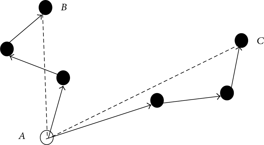
Idea of Lin's algorithm.

In Figure 1, node A   represents an unknown node, and the solid nodes represent some anchors. Node A can use anchor B and anchor C to calculate the location itself. In DV-Hop, network uses the distance between node A and anchor B and the distance between node A and anchor C, both of which are $3\mathrm{\ast }R$ (R is the communication radius). However, the distance between node A and anchor C is obviously closer to $3\mathrm{\ast }R$ than that between node A and anchor B; therefore the error of using anchor B is bigger than that of using anchor C. The authors of Lin's algorithm find out more suitable anchors by fitting a preset curve, and then they can obtain more accurate locations. The method to find better anchors is shown as the following expression:

$$\begin{array}{cc}& \text{MIN}\left(\sqrt{\frac{{\sum }_i^n{\left(x_i-x\right)}^{\mathrm{2}}+{\sum }_i^n{\left(y_i-kx\right)}^{\mathrm{2}}}{n}}\right).\end{array}$$

(1)

In expression (1), ( $x,k\mathrm{\ast }x$ ) stands for the preset curve and ( $x_i,y_i$ ) stands for the anchors which are near the curve, a preset straight line. The result comes from calculating the minimum square root of the distance between anchors of given scope and the straight line. For example, in Figure 1, node A will choose anchor C rather than anchor B.

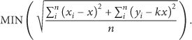
However, our experiments on comparing Lin's algorithm with DV-Hop show that the localization accuracy of Lin's algorithm is not better than DV-Hop in some cases. The reason is shown as in Figure 2.

Figure 2

Disadvantage of Lin's algorithm.

In Figure 2, the black filled nodes stand for anchors, and node A stands for an unknown node, and the black node D stands for a special node which is excluded by node A. Node A can select anchor C rather than anchor B as a referential anchor. If DV-Hop or weighted DV-Hop also selects node C randomly, the localization results of node A using DV-Hop, weighted DV-Hop, and Lin's algorithm will be the same, because even though node A excludes node D, anchor C still cannot communicate with anchor E directly without node D as a relay node. The distance between anchor C and anchor E is longer than R, so the distance between anchor C and anchor E is still $2\mathrm{\ast }R$ .

We propose an improved localization algorithm based on amendatory simulation curve fitting (ASCF) in this paper, which makes anchor selection process more reasonable and calculates the distance between different nodes more precisely. When selecting a reference anchor, an unknown node will not only filter the suitable anchors by fitting them to a preset curve but also calculate the real distance between two particular anchors by ASCF. Compared with other algorithms, ASCF can improve the localization accuracy effectively.

3. Proposed Algorithm: Amendatory Simulation Curve Fitting (ASCF)

3.1. Principles of ASCF

Considering the above analysis, we can select more suitable anchors using Lin's algorithm [10]. But the error of the distance between selected anchor and unknown node is the same as DV-Hop in some cases. We propose ASCF algorithm to fix this problem.

In ASCF, each unknown node selects three anchors from its neighbor anchors or from those within its two hops' distance. Then, network can obtain a curve on the selected anchors. According to this curve, network can select more suitable anchors and calculate the exact distance between the two anchors. And then network can move the selected anchors and estimate the distance between the unknown node and the far-side anchor so that the error of the localization can be decreased. The calculation formula is

$$\begin{array}{cc}& D_k=\sqrt{{\left(x_i-x_j\right)}^{\mathrm{2}}+{\left(y_i-y_j\right)}^{\mathrm{2}}}+\text{HopSiz}{\text{e}}_k.\end{array}$$

(2)

In formula (2), $D_k$ is the distance between unknown node k and the selected anchor node. ( $x_i,y_i$ ) is the coordinate value of the anchor node within communication radius of k. ( $x_j,y_j$ ) is a selected anchor node far away from K, and ${\text{HopSize}}_k$ is the average hop size of k. For example, in Figure 3, star node stands for an unknown node, black filled node stands for anchors, and circle node stands for the position of anchors after being moved. Node a is a selected anchor in the localization procedure of the unknown node A. We draw a straight line K from the original node to anchor a and use line K to select the anchor B which is the closest one to line K, and then we move anchor a to node c changing its horizontal ordinate and vertical ordinate by ( $d_1,d_2$ ), respectively. After that, we draw a parallelogram by connecting anchor a, node c, and anchor B to obtain node d. Now node d is the new position of anchor B after being moved. Then the estimated distance between unknown node A and anchor B is the distance between node c and node d adding R (communication radius) of unknown node A. In this way, the distance between the unknown node and the selected anchor is more accurate so that we can use these data in trilateration to reduce the error of the localization algorithm in WSN.

Figure 3

ASCF idea diagram.

Furthermore, we design the ASCF algorithm to reduce energy consumption by decreasing the communication times. We design more reasonable steps of the algorithm including the step of selecting more suitable anchors to reduce energy consumption. The detailed design is described in the next section.

3.2. Flowchart of ASCF Algorithm

Now we explain the ASCF localization algorithm step by step as follows. This improved algorithm is researched on the basis of DV-Hop and Lin's algorithm. So these algorithms have some similar steps during calculation stage.

Step 1.

Deploy sensor nodes randomly in given monitoring area.

Step 2.

Localize all of the anchors by GPS.

Step 3.

Anchors broadcast their own location information in the whole network and set the counter value as 0.

Step 4.

Unknown nodes receive the location and hops' information from anchors and then find out and record the information with the fewest hops. Each unknown node arranges all the anchors by hops.

Step 5.

Set $K\mathrm{\ast }R$ as the radius of the candidate area; R is communication radius and K is adjusting parameter. This is to insure that at least three anchors exist in candidate area.

Step 6.

According to the hops from the anchors, each unknown node selects the anchor that is nearest to it within candidate area. For example, an unknown node N obtains the information of an anchor ( $x_i,y_i$ ) randomly in candidate area and selects one anchor A randomly among all of the anchors outside of candidate area which transfer information through anchor ( $x_i,y_i$ ). Then, the unknown node records the information of the two anchors.

Step 7.

Each unknown node selects the second anchor from the left anchors. This anchor must be the one that is nearest to the unknown node and is within candidate area. For example, unknown node N obtains an anchor ( $x_j,y_j$ ) randomly in candidate area rather than anchor ( $x_i,y_i$ ) and selects another anchor B excluding anchor A by the same way mentioned in Step 6 and then records anchor ( $x_j,y_j$ ) and anchor B.

Step 8.

Each unknown node selects the third anchor from the left anchors. This anchor must be the one that is nearest to the unknown node and is within candidate area. For example, unknown node N obtains an anchor ( $x_k,y_k$ ) randomly in candidate area rather than anchor ( $x_i,y_i$ ) and anchor ( $x_j,y_j$ ) and selects the third anchor C excluding anchor A and anchor B by the same way mentioned in Step 6 and then records anchor ( $x_k,y_k$ ) and anchor C.

Step 9.

Unknown nodes obtain three estimated distance values between themselves and anchors A, B, and C. These three values are used to calculate the unknown nodes' locations using trilateration method. The three estimated values of distance are as follows:

• (1)

The first estimated value of distance is “the distance between ( $x_i,y_i$ ) and A” + $K\mathrm{\ast }R$ .

(2)

The second estimated value of distance is “the distance between ( $x_j,y_j$ ) and B” + $K\mathrm{\ast }R$ .

(3)

The third estimated value of distance is “the distance between ( $x_k,y_k$ ) and C” + $K\mathrm{\ast }R$ .

According to the above discussion, we can draw a conclusion that the selection procedure of referenced anchors in ASCF is more reasonable, and the estimated value of distance between unknown node and the selected anchors in ASCF is more accurate. Furthermore, ASCF broadcasts once, but both DV-Hop and Lin's algorithm broadcast twice, so the energy consumption of ASCF is the fewest. The details of the ASCF flowchart are shown as in Figure 4.

Figure 4

Flowchart of ASCF process.

In Figure 4, there is only one time of broadcast in ASCF. Even though the process of ASCF is similar to DV-Hop, the estimated distance between the unknown node and the selected anchors is more reasonable, and the method of selecting anchors is more rational. So the localization accuracy of localization process can be improved and the energy consumption of algorithm can be reduced. Simulation experiments' results and analytical expatiations are described in the next section.

3.3. Simulation Experiment and Analysis

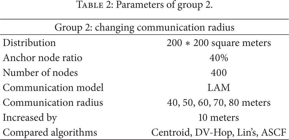
Two groups of experiments are conducted to analyze the performance of ASCF using MATLAB in this paper. In the first group, experiments are carried out based on changing the percentage of the anchors, and in the second group, experiments are based on changing communication radius. The detailed conditions of the two groups are shown as in Tables 1 and 2.

Table 1

Parameters of group 1.

Group 1: changing anchor node ratio
Distribution	$$\mathrm{200}\mathrm{\ast }\mathrm{200}$$ square meters
Anchor node ratio	20%, 30%, 40%, 50%, 60%
Increased by	10%
Number of nodes	400
Communication model	LAM
Communication radius	60 meters
Compared algorithms	Centroid, DV-Hop, Lin's, ASCF

Table 2

Parameters of group 2.

Group 2: changing communication radius
Distribution	$$\mathrm{200}\mathrm{\ast }\mathrm{200}$$ square meters
Anchor node ratio	40%
Number of nodes	400
Communication model	LAM
Communication radius	40, 50, 60, 70, 80 meters
Increased by	10 meters
Compared algorithms	Centroid, DV-Hop, Lin's, ASCF

Regarding localization algorithm of WSN, two parameters can influence localization accuracy crucially. Those two parameters are the percentage of anchors and the communication radius. As shown in Table 1, we compare Centroid algorithm, DV-Hop algorithm, Lin's algorithm, and ASCF algorithm under different percentage of anchors in monitoring area, that is, 20%, 30%, 40%, 50%, and 60%. In Table 2 we compare the four algorithms under different communication radiuses, that is, 40, 50, 60, 70, and 80 meters. By simulation experiment, we evaluate the performances of the four algorithms.

For the comparison of the four algorithms, the experiments are repeated for 5 rounds, and in each round there are 100 times of tests. In the monitored area of $\mathrm{200}\hspace{0.17em}\text{m}\mathrm{\ast }\mathrm{200}\hspace{0.17em}\text{m}$ , 400 sensor nodes are deployed randomly. It is illustrated as in Figure 5.

Figure 5

Network deployment situation.

During the experiments of group 1, we compare the four algorithms on localization accuracy. We choose fixed proportion of anchors and draw the percentage of average localization error of the four algorithms. The result is shown as in Figure 6.

Figure 6

Localization accuracy comparison of group 1.

As Figure 6 shows, communication radius is set as 60 m. After 5 rounds of testing, the average localization error of ASCF is decreased obviously. Localization accuracy of ASCF is improved by about 10% compared with that of Lin's algorithm, 15% compared with that of DV-Hop, and 18% compared with that of Centroid. ASCF method shows that, as the percentage of anchors increases, localization accuracy increases.

In Figure 6, when the percentage of anchors gets higher than 50%, the localization error increases. Regarding this phenomenon, we perform another 17 times of independent experiments to compare the four algorithms. In each time of experiment, 5 rounds of tests are carried out with the anchor percentage parameter set as 20%, 30%, 40%, 50%, and 60%, respectively. In each round of test there are 100 times of localization processing. The experimental results show that the relationship between the changes of percentage of anchors and the changes of localization error is uncertain.

However, in these experiments, 52.94% of cases are that the localization error increases when the percentage of anchors gets higher than 50%. For each unknown node, when the percentage of anchors gets higher than 50%, there might be more neighbor anchors in its communication radius rather than neighbor unknown nodes. Therefore, the error of the estimated distance between unknown node and anchor increases. In detail, when the estimated distance part is $2\mathrm{\ast }R$ , the error is from 0/( $2\mathrm{\ast }R$ ) to $R/(2\mathrm{\ast }R)$ , and the range is [0, 50%), but when the estimated distance part is R, the error is from $0/R$ to $R/R$ , and the range is [0, 100%), so the range of error proportion with big anchor density might be smaller than that with small anchor density. When the percentage of anchors gets higher than 50%, the density of anchors achieves a higher level, and each unknown node can get more neighbor anchors and get larger error range.

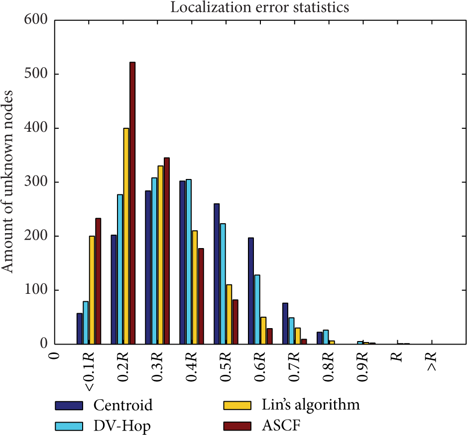
In experiments of group 1, we study on the distribution of the localization error of the four compared algorithms in all the 5 rounds of experiments. The results are shown in Figure 7 to Figure 10. The red bar chart stands for ASCF algorithm, the dark blue bar chart stands for Centroid algorithm, the baby blue bar chart stands for DV-Hop algorithm, and the yellow bar chart stands for Lin's algorithm.

Figure 7

Error distribution with 20% anchors. Error distance ( $R=60\hspace{0.17em}\text{M}$ 20% anchors).

We analyze localization accuracy of different percentage of anchors with fixed communication radius. In Figure 7, the communication radius is set as 60 and the percentage of anchors is set as 20%. As shown in Figure 7, the error of ASCF algorithm mainly exists from $10\%\mathrm{\ast }R$ to $30\%\mathrm{\ast }R$ ; however, the error of Centroid algorithm mainly exists from $30\%\mathrm{\ast }R$ to $50\%\mathrm{\ast }R$ , and the errors of DV-Hop algorithm and Lin's algorithm mainly exist both from $20\%\mathrm{\ast }R$ to $40\%\mathrm{\ast }R$ . So the error of ASCF algorithm is minimal in different percentages of anchors.

In the experiments with 30% anchors, 40% anchors, and 50% anchors, the situations are the same. The experimental results are shown in Figures 8, 9, and 10, and it can be concluded that the error of ASCF algorithm is minimal in each case. Furthermore, the localization error keeps decreasing from $0.2\mathrm{\ast }R$ to R.

Figure 8

Error distribution with 30% anchors. Error distance ( $R=60\hspace{0.17em}\text{M}$ 30% anchors).

Figure 9

Error distribution with 40% anchors. Error distance ( $R=60\hspace{0.17em}\text{M}$ 40% anchors).

Figure 10

Error distribution with 50% anchors. Error distance ( $R=60\hspace{0.17em}\text{M}$ 50% anchors).

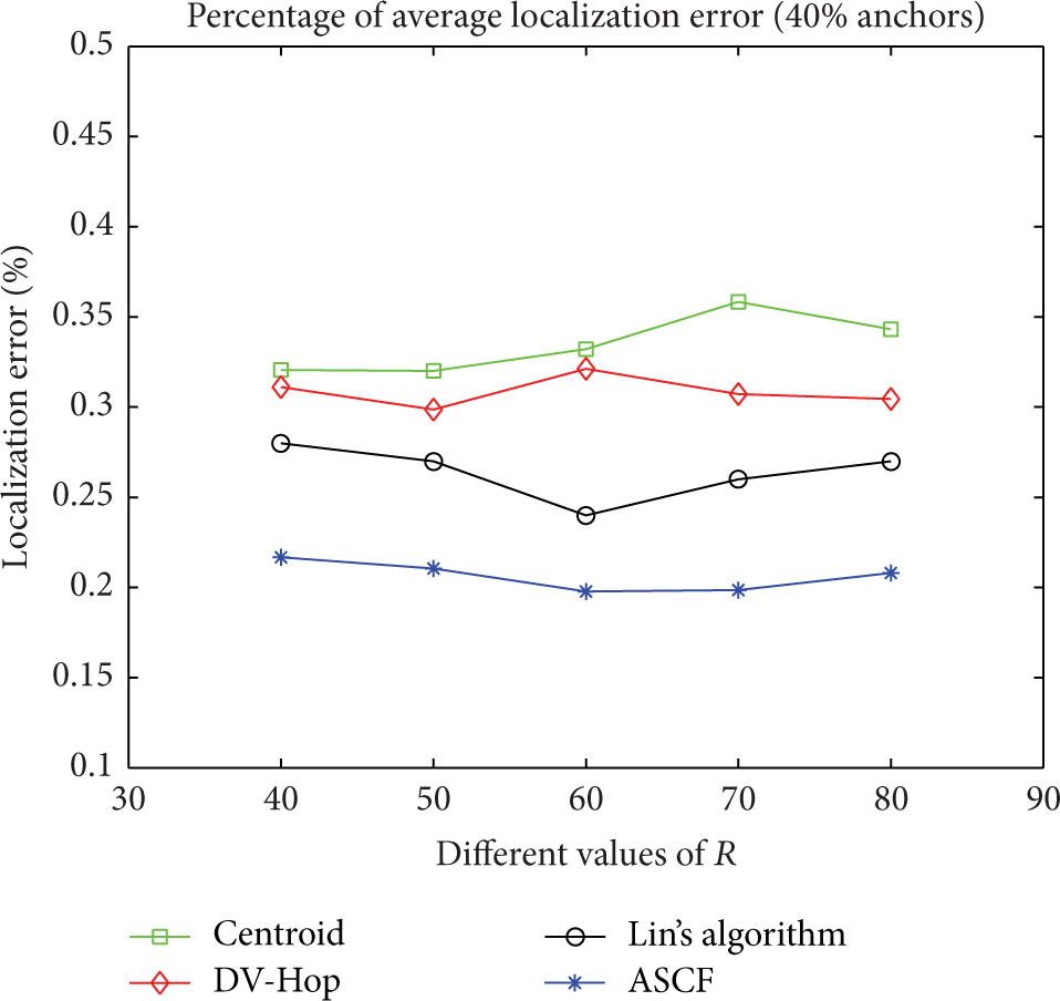
During the experiments of group 2, we compare the four algorithms on the localization accuracy. We choose fixed communication radius and draw the percentage of average localization error of the four algorithms. The result is shown as in Figure 11.

Figure 11

Localization accuracy comparison of group 2.

As shown in Figure 11, the percentage of anchors is set as 40%. After 5 rounds of testing, the average localization error of ASCF is decreased obviously. Localization accuracy of ASCF is improved by about 8% compared with that of Lin's algorithm, 12% compared with that of DV-Hop, and 15% compared with that of Centroid. ASCF shows that as the communication radius increases, the localization accuracy increases. The possibility of the anchors to be neighbor nodes increases when the communication radius enlarges; therefore, the reason of the tendency in Figure 11 is the same as that in Figure 6.

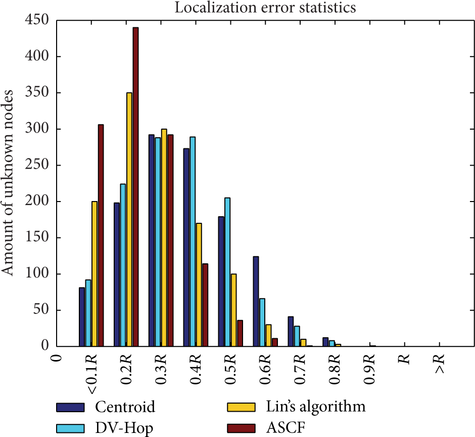
In experiments of group 2, we study on the distribution of the localization error of the four compared algorithms in all the 5 rounds of experiments. The results are shown in Figure 12 to Figure 15, and the red bar chart stands for ASCF algorithm, the dark blue bar chart stands for Centroid algorithm, the baby blue bar chart stands for DV-Hop algorithm, and the yellow bar chart stands for Lin's algorithm.

Figure 12

Error distribution with 40 m communication radius. Error distance (40% anchors $R=40\hspace{0.17em}\text{M}$ ).

We analyze localization accuracy of different communication radius with fixed percentage of anchors. In Figure 12, the communication radius is set as 40 and the ratio of anchors is set as 40%. As shown in Figure 12, the error of ASCF algorithm mainly exists from $10\%\mathrm{\ast }R$ to $30\%\mathrm{\ast }R$ ; however, the errors of Centroid algorithm, DV-Hop algorithm, and Lin's algorithm all mainly exist from $20\%\mathrm{\ast }R$ to $40\%\mathrm{\ast }R$ . So the localization error of ASCF algorithm is less than other algorithms.

In the experiments with 50 m of communication radius, 60 m of communication radius, and 70 m of communication radius, the situations are the same. Experimental results are shown as in Figures 13, 14, and 15, and it can be concluded that the error of ASCF algorithm is also minimal in each case. Furthermore, the localization error also keeps decreasing from $0.2\mathrm{\ast }R$ to R.

Figure 13

Error distribution with 50 m communication radius. Error distance (40% anchors $R=50\hspace{0.17em}\text{M}$ ).

Figure 14

Error distribution with 60 m communication radius. Error distance (40% anchors $R=60\hspace{0.17em}\text{M}$ ).

Figure 15

Error distribution with 70 m communication radius. Error distance (40% anchors $R=70\hspace{0.17em}\text{M}$ ).

4. Conclusion

In WSN, sensor nodes are deployed randomly; therefore, the first step for network to work is to figure out the position of sensor nodes. In this paper, we study localization techniques in WSN. After analyzing DV-Hop and some improved algorithms, we conclude that when searching reference anchors, network calculates the received information from all anchors in monitoring area and broadcasts twice. After that, unknown nodes obtain average hop size and estimated distance between anchors and themselves, both of which lead to localization error. So reference anchors need to be filtered and the estimated distance between unknown nodes and anchor nodes should be corrected.

In this paper, we propose a new localization algorithm based on amendatory simulation curve fitting (ASCF). Each unknown node obtains two optimized parameters, one is the estimated distance between the reference anchor and itself, and the other is the exact distance between the selected anchor and the reference anchor. Each unknown node records at least three pairs of selected anchors and reference anchors all of which are found out using ASCF. After that, unknown nodes can obtain more accurate position using trilateration. Simulation experiments show that ASCF can improve localization accuracy efficiently.