MIDAS: A Data Aggregation Scheduling Scheme for Variable Aggregation Rate WSNs

Abstract

Data aggregation scheduling for variable aggregation rate model has wide application and should take network lifetime and energy efficiency into consideration. In this paper, the time-slot scheduling problem for the variable aggregation rate model is presented, and a time-slot scheduling integrating consideration of minimizing the energy consumption named Makeup Integer based Data Aggregation Scheduling (MIDAS) is proposed. The proposed MIDAS scheme integrates two core phases, namely, data aggregation set construction and aggregation set based scheduling algorithm. The key idea of MIDAS is to minimize the number of receiving and sending data packets in hotspot and to reduce the number of aggregated packets in network for better scheduling performance in network lifetime. Furthermore, it is also essential to increase energy utilization efficiency of the nodes in the middle layer by exploiting the remaining energy of peripheral nodes. A series of experiments are simulated to demonstrate that the proposed scheme has significantly increased the network lifetime and the energy utilization efficiency under the different aggregation rates and different network scales. Comparing with the SDAS, the lifetime can be increased by as much as 25%. The energy utilization efficiency can be improved by as much as 30%.

1. Introduction

Wireless sensor networks (WSNs) have captured considerable attention recently due to their enormous potential for environmental monitoring, surveillance operations, and industrial automation [1–5]. In wireless sensor networks, data aggregation is an important method of improving transmitting efficiency, and most existing researches have mainly focused on energy consumption [6–11] or transmission latency [12–19]. Some works have investigated the energy latency tradeoff [20–22].

In most past researches, data aggregation refers to the situation in which data packets meet at a node in the routing procedure and they are aggregated into one new data packet. Based on the assumption of transmitting one data packet in one time-slot, each node needs only one time-slot to transmit this one data packet. In real-life application, n nodes are aggregated into multidata packets. So multislots need to be assigned for one node, which may result in the allocation complexity of time-slot scheduling. And the following factors should be comprehensively considered.

(1) Interference. Each sensor is equipped only with a single radio transceiver, sending and receiving cannot be carried out simultaneously. The interference range r is the maximum distance within which nodes in receiving mode will be disturbed by an unrelated transmitter, thus suffering a loss. If a node hears more than one message at the same time, it can receive none of them correctly; therefore this causes a collision. Thus, two links are interfering if the receiver of at least one link is within the range of the transmitter of the other link.

(2) Time Constraints. Node scheduling should obey a sequential order. The time-slots are not necessarily continuously allocated for one node. A time-slot can be used for different purposes. It can be used to transmit its original data as well as the aggregated data. It can also be used to transmit other nodes' original data as well as the aggregated data. Thus, how to allocate multislots for one node will be a challenging issue.

(3) Energy Consumption. Because of the limitability of energy in WSNs, the energy consumption of sensor nodes should be considered in the process of data transmission [23–25]. Therefore, it is our major concern how to design an effective TDMA based aggregation scheduling algorithm, which can minimize the number of receiving and sending data packets in network to optimize the energy of WSNs.

Therefore, it is a challenge to study on data aggregation scheduling combining time-slot and variable aggregation rate. The main contributions of our work are as follows.

(1) This paper addressed the time-slot scheduling problem for the variable aggregation rate model. In the model, each node aggregates the original data of its child nodes and its own original data based on the given aggregation rate and then packs the aggregation result into m new data packets ( $m\in [\mathrm{1},n]$ ) and forwards them.

(2) This paper presented a Makeup Integer based Data Aggregation Scheduling (MIDAS) integrating to minimize the energy cost. Based on the aggregation model and the given aggregation rate, we select some nodes to construct multiple aggregation sets so that the size of each set is as close to its round-up integer as possible. And then the number of aggregated packets in the network is reduced for better scheduling performance. This method can decrease the energy consumption near the sink, increase the energy utilization efficiency, and improve the network lifetime. The key challenge is then to construct aggregation set. The aggregation set guarantees each node to aggregate once in the set. The nodes within the same aggregation set aggregate at the aggregation node in one sample cycle. And the nodes except aggregation node only forward the data from the upper stream sensors in the aggregation set. After the establishment of the aggregation set, the next step is to solve the problem of time-slot scheduling. In the schedule algorithm, the nodes in hotspots would hold on transmission and accumulate their data before sending them to sink at once.

Constructing the aggregation set with a round off thought can reduce the number of the aggregated data packets of the nodes in the first layer near the sink and decrease the energy consumption of the nodes in this area. For no aggregated nodes in the area far from the sink, the number of transmission data is not smaller but more than that near the sink. Thus, the remaining energy far away from the sink is fully utilized, which increases the energy utilization efficiency of the nodes in the middle layer and improve the energy utilization efficiency of the network.

(3) The results of simulation on the random generated tree topologies show that the time-slot scheduling proposed in this paper could realize the dual goals of improving the network lifetime and increasing energy efficiency. Comparing with the simple time-slot scheduling, the lifetime can be improved by as much as 25%. The energy utilization efficiency can be increased by as much as 30%.

The rest of this paper is organized as follows: In Section 2, the related works are reviewed. In Section 3, we discuss the research motive. The system model is described in Section 4. In Section 5, a data aggregation scheduling scheme for variable aggregation rate is presented. The simulation results and performance are analyzed in Section 6. Finally, we conclude in Section 7.

2. Related Work

The current data aggregation scheduling schemes are discussed in this section. Most previous works have mainly focused on energy-saving issue and it has been investigated in [6–11]. Krishnamachari et al. [6] illustrated the impact of data aggregation by comparing its performance with traditional end-to-end routing schemes. Wu et al. [8] used TDMA as the MAC layer protocol and scheduling the sensor nodes with consecutive time-slots at different radio states while reducing the number of state transitions. Wen et al. [9] proposed Heuristics for cluster construction and data aggregation routing such that total energy consumption is minimized. Mo et al. [10] presented a stochastic sensor selection algorithm that randomly selects a subset of sensors according to a certain probability distribution. Li et al. [11] proposed a connected dominating set based transmission scheduling algorithm. There are some papers that build a data aggregation tree to control the delay in [12–19]. The minimum-latency data aggregation problem (MDAT) in wireless sensor networks is well studied and proved to be NP hard [12]. Chen et al. had designed an approximation algorithm with the delay bound of $(\Delta -\mathrm{1})R$ for this problem, where Δ is the maximum node degree and R is the network radius. Huang et al. [13] proposed a centralized scheduling algorithm with the delay bound of $23R+\Delta +18$ time-slots. Wan et al. [14] extended the result in Huang et al. and designed three types of aggregation scheduling for $\rho =1$ with latency bound $\mathrm{15}R+\Delta -\mathrm{4}$ , $\mathrm{2}R+O(\log R)+\Delta$ , and $(\mathrm{1}+O(\log R/\sqrt[\mathrm{3}]{R}))R+\Delta$ , respectively, where ρ is an interference radius. Yu et al. [15] proposed a distributed aggregation transmission scheduling algorithm with the delay bound of $\mathrm{24}D+\mathrm{6}\Delta -\mathrm{16}$ time-slots, where D is the network diameter. Xu et al. [16, 17] theoretically proved that the delay of the aggregation scheduling generated by their algorithm is at most $16R+\Delta -14$ time-slots. Wang et al. [18] designed a scheduling algorithm, Peony-tree based data aggregation (PDA), and proved the latency bound is $\mathrm{15}R+\Delta -\mathrm{15}$ . Zhang et al. have proposed distributed network estimation and decentralized aggregation scheduling algorithm [19]. It could predict the upper stream sensors' estimates which cannot be aggregated to the sink before deadlines and it is able to aggregate as much estimate information as possible from the network to the sink within delay constraints. Some works have investigated the energy latency tradeoff [20–22]. Given a deadline, they minimized the amount of missed data [20], minimized overall energy dissipation of sensor nodes [21], or minimized the maximum energy consumption [22].

However, the abovementioned algorithms are all based on the assumption that data packets from n nodes can be aggregated into one data packet or n data packets and study the time-slot scheduling under these models [26, 27]. They are not suitable for the network with variable aggregation rate.

3. Research Motivation

The tree topology of a random network with 25 nodes rooted at the sink is illustrated in Figure 1. And the node ID is marked in the figure. The arrow line represents data transmission paths and the dashed line indicates the transmission interference.

Figure 1

A randomly generated aggregation tree with 25 nodes.

Having the minimum scheduling period of one hop node set $C=\mathrm{4}$ , the node scheduling time-slot is assigned with the algorithm proposed in [19]. Table 1 illustrates the scheduling results. Column represents the node's ID, ( $x,y$ ) represent time-slot scheduling, where x denote the assigned time-slot at which node ID sends its data to its parent for the first time. y denote node scheduling period.

Table 1

The time-slot assignment for all nodes.

ID	1	2	3	4	5	6	7	8	9
( $x,y$ )	×	(2, 4)	(4, 4)	(1, 4)	(3, 4)	(1, 4)	(3, 8)	(7, 8)	(4, 4)
ID	10	11	12	13	14	15	16	17	18
( $x,y$ )	(7, 8)	(5, 8)	(1, 8)	(3, 8)	(1, 4)	(2, 4)	(1, 8)	(2, 8)	(8, 8)
ID	20	21	22	23	24	25	×	×	×
( $x,y$ )	(6, 8)	(1, 4)	(3, 4)	(1, 8)	(3, 8)	(1, 8)	×	×	×

The data aggregation mechanism in [19] is based on the assumption that data packets of n nodes can be aggregated into one data packet. But if the aggregated data packets are more than one, and then there have some problems as follows.

(1) A node can not only be assigned one time-slot, but also may require multiple time-slots, which will make time-slot scheduling more complicated.

For instance, there exit two data packets that are produced by node 18 after the aggregation computation by the original data of node 18, node 23, and node 24. It must be assigned two time-slots to node 18 for transmission of the two data packets. And there are two data packets that are produced by node 10 after the aggregation computation by the original data of node 10, node 16, and node 17. It must be assigned two time-slots to node 10 for transmission of the two data packets. In addition, node 10 also needs to transmit the aggregation result of its child node 18. Thus we need to assign four time-slots totally for node 10.

Therefore, previous research methods assigning only one time-slot for one node cannot be adapted to the case where n nodes are aggregated into multidata packets. How to allocate multiple time-slots for one node to transmit its own original or aggregated data as well as its child nodes' original or aggregated data will be a challenging problem.

(2) How to design an effective aggregation scheduling algorithm which can balance the energy consumption is an important issue. Furthermore, it is also essential to increase energy utilization efficiency and prolong the network lifetime by exploiting the remaining energy of peripheral nodes.

We consider the subtree rooted at node 13 in Figure 1. Several typical aggregation scheduling approaches are selected for this explanation and the data aggregation rate is 0.25 for every node. The first is as shown in Figure 2(a), assuming that one data packet is produced by node 13 after the aggregation computation by the original data of nodes 13, 19, 20, and 25. It must be assigned one time-slot to node 13 for transmission of the one data packet. The second is as shown in Figure 2(b), assuming that one data packet is produced by node 13 after the aggregation computation by the original data of node 13 and node 19. And one data packet is produced by node 20 after the aggregation computation by the original data of node 20 and node 25. It must be assigned two time-slots to node 13, where one time-slot is used to transmit the aggregation result of itself, and another is used to transmit the aggregation result of its child node 20. The third is as shown in Figure 2(c); one slot is assigned for node 13 to send its own data, one slot is assigned to transmit the data of node 19, and one slot is assigned to transmit the aggregation result of its child node 20; that is, three slots are required for node 13. The forth is as shown in Figure 2(d); one slot is assigned for node 13 to send its own data, and three slots are assigned to transmit the data of nodes 19, 20, and 25, respectively; that is, four slots are required for node 13. The digital above the arrows represents the number of packets being sent in Figure 2.

Figure 2

Several typical aggregation forms of node 13.

Assume ${\varpi }_t^i$ denotes the number of transmitting data packets of node i. ${\varpi }_r^i$ denotes the number of receiving data packets of node i. ${\tau }_i$ denotes the number of slots required for node i. And, in Figures 2(a), 2(b), 2(c), and 2(d), their corresponding values are shown in Figure 3.

Figure 3

The results of an instance under different cases.

As can be seen from Figure 3, the number of receiving and sending data packets of node 13 is different when exploiting different aggregation scheduling approaches, which leads to the different number of slots required for node 13. It is obviously that the more number of forwarding packets causes the more energy cost. We can see from Figure 3 that node 13 will receive three data packets and send one data packet by exploiting the method shown in Figure 2(a). Therefore, the number of sending data packets of node 13 is the least and the energy consumption also is the lowest. So, if we design an aggregation scheduling approach which can reduce the number of receiving and sending data packets near the sink and increases the number of the transmitting data packets far away from the sink, it will balance the energy consumption and thus prolong the network lifetime.

4. The System Model and Problem Statement

4.1. Network Model

We consider a wireless sensor network $G(V,E)$ with tree topology rooted at the sink, which is constructed by using the BFS method or by other methods proposed in [15], where V is the set of nodes and E is the set of communication links. We assume that all nodes once deployed are not movable and have the same communication range r and the same initial energy. In the protocol interference model [28] on which our work is based, each node has only one transmitting frequency and it cannot send and receive data simultaneously. For any node V, it has an interference range R. As shown in (1), a receiver V of a link VU is interfered by the signal from another node P. Consider the following:

$$\begin{array}{cc}& ‖V-P‖\le R.\end{array}$$

(1)

In this paper, nodes are called one hop neighbors if there exits interferences between them. To ensure data transmission interference free, when any node is receiving data at any one timeslot, the other one hop neighbors cannot send data except to one of child nodes. And, when any node is sending, the other one hop neighbors cannot receive packets except from its parent node. We assume that the relationship between one hop neighbors except parent-child nodes is indicated by dashed lines in the aggregation tree (the same in the following).

4.2. Energy Consumption Model

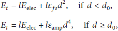
The energy consumption model in this paper is the same as [29]. The energy cost when a node sends l bits data is computed by (2). The energy cost when a node receives l bits data is computed by (3). Consider the following:

$$\begin{array}{cc}& E_t=l{E}_{\mathrm{e}\mathrm{l}\mathrm{e}\mathrm{c}}+l{\epsilon }_{fs}{d}^{\mathrm{2}},\hspace{1em}\mathrm{i}\mathrm{f}\hspace{0.17em}\hspace{0.17em}d<d_{\mathrm{0}},\\ E_t=l{E}_{\mathrm{e}\mathrm{l}\mathrm{e}\mathrm{c}}+l{\epsilon }_{\mathrm{a}\mathrm{m}\mathrm{p}}{d}^{\mathrm{4}},\hspace{1em}\mathrm{i}\mathrm{f}\hspace{0.17em}\hspace{0.17em}d\ge d_{\mathrm{0}},\end{array}$$

(2)

$\begin{array}{cc}& E_r=E_r\left(l\right)=l{E}_{\mathrm{e}\mathrm{l}\mathrm{e}\mathrm{c}}.\end{array}$

(3)

$E_{\mathrm{e}\mathrm{l}\mathrm{e}\mathrm{c}}$ denotes the transmitting circuit loss energy. Both the free space ( $d^{\mathrm{2}}$ power loss) and the multipath fading ( $d^{\mathrm{4}}$ power loss) channel models are used. If the transmission distance is less than the threshold $d_{\mathrm{0}}$ , the power amplifier loss is based on free-space model. If the transmission distance is larger than or equal to the threshold $d_{\mathrm{0}}$ , the multipath attenuation model is used. ${\epsilon }_{fs}$ and ${\epsilon }_{\mathrm{a}\mathrm{m}\mathrm{p}}$ are the energy required by power amplification in the two models. l is the number of bits in a packet.

4.3. Data Aggregation Model

For each sample cycle, all sensor nodes do sampling once. At the beginning of each sample period, each sensor node generates a packet with the sensed information. The sample period is composed of multiple integer timeslots. And we assume the source data packet of each node is generated synchronously. Actually, one data packet needs to be transmitted in one time-slot. If the calculated data packet size is less than that of one packet after aggregation, we should transmit it as one data packet. And the transmission of one data packet must be finished in one time-slot. Therefore, 1.25 packets require two time-slots for transmission and 2.5 packets need three time-slots for transmission.

Definition 1 (the number of data packets ϖ).

$\xi (m{)}_i$ denotes the total amount of data produced at node i after the aggregation computation by node i and other $m-\mathrm{1}$ nodes. D denotes the amount of information contained in each data packet. The number of data packets ${\varpi }_i$ that node i is transmitting is computed by

$$\begin{array}{cc}& {\varpi }_i=⌈\frac{\xi {\left(m\right)}_i}{D}⌉.\end{array}$$

(4)

Namely, data packet ${\varpi }_i$ is the rounding-up ratio of the total amount of data $\xi (m{)}_i$ and the amount of information contained in each data packet D.

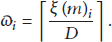
Definition 2 (data aggregation rate γ).

γ denotes data aggregation rate which is a decimal between 0 and 1. For example, $\gamma =0.5$ . Traditionally, n nodes are aggregated into one packet (as grey nodes shown in Figure 4, the boxes above the arrows represent the number of packets being sent). Given γ, n nodes can be aggregated into m data packets. m is an integer, $m\in [\mathrm{1},n]$ (as green nodes shown in Figure 4).

Figure 4

Data aggregation model.

Definition 3 (aggregation model).

For data aggregation, one adopts the lossless step-by-step multihop aggregation model. In such aggregation model, ${\sigma }_i$ denotes the original data packet of node i, ${\phi }_{i,j}$ denotes the received data packet of node i from node j, and ${\varphi }_i$ denotes the final aggregation result of node i to all incoming data and its own data.

When node i receives data ${\phi }_{i,j}$ from node j, if current data packet of node i is ${\sigma }_i$ , and data from j is ${\phi }_{i,j}={\sigma }_j$ , namely, the data to be aggregated is both origin data, then the aggregation formula follows

$$\begin{array}{cc}& {\varphi }_i={\sigma }_i\times \gamma +{\phi }_{i,j}\times \gamma .\end{array}$$

(5)

If the current data packet of node i is ${\sigma }_i$ , and data from j is ${\phi }_{i,j}={\varphi }_j$ , namely, the received data packet of node i is not source data when being aggregated, the aggregation formula follows

$$\begin{array}{cc}& {\varphi }_i={\sigma }_i\times \gamma +{\phi }_{i,j}.\end{array}$$

(6)

For example, as green nodes depicted in Figure 4, we assume that the packet size is $5\ast {10}^5$  bits, when $\gamma =0.5$ ; according to (4), (5), and (6), we get

$$\begin{array}{cc}& {\varphi }_A={\sigma }_A\times \mathrm{0.5}+{\sigma }_B\times \mathrm{0.5}+{\phi }_{A,C},\\ {\phi }_{A,C}={\varphi }_C={\sigma }_C\times \mathrm{0.5}+{\sigma }_D\times \mathrm{0.5}+{\sigma }_E\times \mathrm{0.5}.\end{array}$$

(7)

The number of data packet needs to be transmitted by node C as in the following:

$$\begin{array}{cc}& {\varpi }_C=⌈\frac{\left({\sigma }_C+{\sigma }_D+{\sigma }_E\right)\times \gamma }{D}⌉=⌈\frac{\left(\mathrm{5}\ast {\mathrm{10}}^5+\mathrm{5}\ast {\mathrm{10}}^5+\mathrm{5}\ast {\mathrm{10}}^5\right)\times \mathrm{0.5}}{\mathrm{5}\ast {\mathrm{10}}^5}⌉=\mathrm{2}.\end{array}$$

(8)

Thus, we need to assign two time-slots for node C. The number of data packet needs to be transmitted by node A as in the following:

$$\begin{array}{cc}& {\varpi }_A=⌈\frac{\left({\sigma }_A+{\sigma }_B\right)\times \gamma }{D}⌉+{\varpi }_C=⌈\frac{\left(\mathrm{5}\ast {\mathrm{10}}^5+\mathrm{5}\ast {\mathrm{10}}^5\right)\times \mathrm{0.5}}{\mathrm{5}\ast {\mathrm{10}}^5}⌉+\mathrm{2}=\mathrm{3}.\end{array}$$

(9)

Therefore, node A needs to be assigned three time-slots for transmitting the three packets.

4.4. Problem Statements

The objective is to design a Data Aggregation Scheduling (MIDAS) scheme for variable aggregation rate WSNs. The scheduling time of the node i is denoted by $Tsf{t}_j$ . When being first scheduled, the relay node transmits its own original data packet to its parent directly. The aggregation node aggregates its own data with data received from its child nodes, and then it transmits the aggregated data packets to its parent directly. In other scheduled time slots, all nodes forward the received data from their related child nodes to parents.

We use the energy cost model presented in Section 4.2 to calculate the network energy consumption. In this paper, network lifetime is defined as the time when the first node dies. After the first node dies in the network, it could seriously affect the connectivity and coverage of network, so that the network cannot fully play its due role. Considering all nodes in the network, the network lifetime is represented by (10), where $E_i$ represents the energy consumption of node i, and T denotes the network lifetime. Consider the following:

$$\begin{array}{cc}& T=\underset{\mathrm{0}<i\le n}{\mathrm{m}\mathrm{i}\mathrm{n}}\left(E_i\right).\end{array}$$

(10)

The energy utilization efficiency is defined as the ratio of the utilized energy to initial energy when the network dies. The energy utilization efficiency is represented by (11), where $E_{\mathrm{c}\mathrm{o}\mathrm{n}\mathrm{s}}^i$ represents the energy consumption of node i.

$E_{\mathrm{i}\mathrm{n}\mathrm{i}\mathrm{t}}^i$ denotes the initial energy of node i and η denotes the energy utilization efficiency:

$$\begin{array}{cc}& \eta =\frac{{\sum }_{i\in n}^{}{E}_{\mathrm{c}\mathrm{o}\mathrm{n}\mathrm{s}}^i}{{\sum }_{i\in n}^{}{E}_{\mathrm{i}\mathrm{n}\mathrm{i}\mathrm{t}}^i}.\end{array}$$

(11)

There is a complex relationship among transmitting data packet, energy consumption of nodes, and network lifetime. So we try to reduce data packets transmitted in the network, especially packets in the area near the sink. In the schedule algorithm, the nodes in hotspots would hold on transmission and accumulate their data before sending them to sink at once. This could realize the dual goals of increasing the amount of information aggregated to sink and decreasing the number of the transmitting data packets in network. Thus, according to (4) in Section 4.3, we select m packets to aggregate at the aggregation node i, the minimum value of m is represented by

$$\begin{array}{cc}& \min \left(m\right)=\min \left(⌈\frac{\xi {\left(m\right)}_i}{D}⌉-\frac{\xi {\left(m\right)}_i}{D}\right).\end{array}$$

(12)

The work of schedule is to assign multiple time-slots to each node in the network to ensure interference free and the network lifetime maximization and the energy utilization efficiency maximization. In conclusion, the optimization goal of this paper is expressed in the following formula, where $E_{\mathrm{l}\mathrm{e}\mathrm{f}\mathrm{t}}^i$ represents the residual energy of node i:

$$\begin{array}{cc}& \max \left(T\right)=\mathrm{m}\mathrm{i}\mathrm{n}\hspace{0.17em}\underset{\mathrm{0}<i\le n}{\max }\left(E_i\right),\\ \max \left(\eta \right)=\min \left(\frac{{\sum }_{i\in n}^{}{E}_{\mathrm{l}\mathrm{e}\mathrm{f}\mathrm{t}}^i}{{\sum }_{i\in n}^{}{E}_{\mathrm{i}\mathrm{n}\mathrm{i}\mathrm{t}}^i}\right),\\ \min \left(m\right)=\min \left(⌈\frac{\xi {\left(m\right)}_i}{D}⌉-\frac{\xi {\left(m\right)}_i}{D}\right).\end{array}$$

(13)

5. Scheme Design

5.1. Construct the Aggregation Set of Nodes

Definition 4 (aggregation set).

Given an integer m and a series set $S=\{S_{\mathrm{1}},S_{\mathrm{2}},\dots ,S_k\}$ , $\forall S_i\subset S,\hspace{0.17em}\hspace{0.17em}{L}_i\le m,\hspace{0.17em}\hspace{0.17em}{\bigcup }_{i=\mathrm{1}}^k{S}_i=\left\{\mathrm{1,2},\dots ,n\right\}$ , n is a sensor node in WSNs, and $L_i$ is the number of $S_i$ contained. We call an aggregation set if and only if $\mathbf{\forall }{S}_i,\hspace{0.17em}{S}_j\subset S,\hspace{0.17em}{S}_i\cap S_j=\varphi$ . $S_i$ is called an aggregation set. For instance, when γ = 30%, $S=\{S_{\mathrm{1}},S_{\mathrm{2}},\dots ,S_k\}$ is shown in Figure 5(c). The colored nodes mean that they are in different $S_i$ .

Figure 5

The aggregation set results of Figure 1.

Characteristic 1. If $L_i\ne \mathrm{1},\hspace{0.17em}\hspace{0.17em}\exists x\in S_i,\hspace{0.17em}\hspace{0.17em}\forall y\in S_i,\hspace{0.17em}\hspace{0.17em}x\ne y$ , y is a child-node in subtree rooted at x. x is the aggregation node; it will aggregate its own original packets with received packets from its child nodes in $S_i$ into new data packets and then transfers it out. y is a relay node; it will only send its own data packet and forward received packets to its parent without aggregation.

Characteristic 2. According to the Characteristic 1, we know that, $\forall x\in S_i$ , if z is a child-node in subtree rooted at x and z is an aggregation node in $S_j,\hspace{0.17em}\hspace{0.17em}i\ne j$ , then x will only forward the aggregation result of z without aggregation repeat.

Our aggregation scheduling algorithm is based on an aggregation tree. Assume the maximum level number of the aggregation tree is H. $L_i$ denotes nodes in each layer i. For example, from Figure 1, we can see that the sink node is in the layer 0; nodes 6, 7, 8, and 9 are in layer 2. There are totally 5 layers in this example.

According to (12) in Section 4.4, we can get

$$\begin{array}{cc}& \exists M_{\mathrm{0}}\in \left[\mathrm{1,2},\mathrm{3},\dots ,n\right],\\ \underset{m\to M_{\mathrm{0}}^{-}}{\mathrm{l}\mathrm{i}\mathrm{m}}\gamma \times m=N,\\ \hspace{1em}N\in \left[\mathrm{1,2},\mathrm{3},\dots ,n\right],\end{array}$$

(14)

where $M_{\mathrm{0}},N,m$ are integers and $N,m$ are minimum values to satisfy (14). In the actual network, if the number of nodes is less than m and then we select $m^{\prime }$ nodes to construct a set, $m^{\prime }$ is close to m.

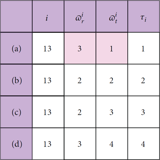
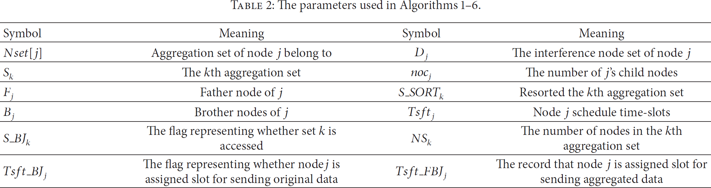
The parameters used in Algorithms 1–6 are as shown in Table 2. Consider $j\in [\mathrm{1},n]$ , $k\in [\mathrm{1},K]$ .

Table 2

The parameters used in Algorithms 1–6.

Symbol	Meaning	Symbol	Meaning
$$Nset[j]$$	Aggregation set of node j belong to	$$D_j$$	The interference node set of node j
$$S_k$$	The kth aggregation set	$$no{c}_j$$	The number of j's child nodes
$$F_j$$	Father node of j	$$S\_SOR{T}_k$$	Resorted the kth aggregation set
$$B_j$$	Brother nodes of j	$$Tsf{t}_j$$	Node j schedule time-slots
$$S\_B{J}_k$$	The flag representing whether set k is accessed	$$N{S}_k$$	The number of nodes in the kth aggregation set
$$Tsft\_B{J}_j$$	The flag representing whether nodej is assigned slot for sending original data	$$Tsft\_FB{J}_j$$	The record that node j is assigned slot for sending aggregated data

Algorithm 1: Constructing the aggregation set (CAS).

$(1)$ Obtain m according to (14),

$(2)$ Set $K\leftarrow \mathrm{1}$ ; $S_k\leftarrow \phi$ ; $Nset[j]\leftarrow \mathrm{0},j\in (\mathrm{1},n)$ ;

(3)   FOR $i\in [H,\mathrm{1}]$    // i denote the ith layer

$(4)$  FOR each node $j\in L_i$

(5)  IF  node $j\notin \left\{S_k\hspace{0.17em}|\hspace{0.17em}k\in \left[\mathrm{1},K\right]\right\}$   $//$ if node j is not in any $S_k$

(6)    $k\leftarrow K$ ; // k denote the kth aggregation set

(7)    $S_k\leftarrow S_k\cup \{j\}$ ;  // put node j in $S_k$

(8)    $Nset[j]\leftarrow k$ ;   // j belong to the kth aggregation set

$(9)$    calculate the number of nodes L in set $S_k$ ;

( $10$ )   While   $L<m$

( $11$ )    Call Search_fnode( $j;S_k;K;Nset;m$ );

(12)    Call Search_bnode( $j;S_k;K;Nset;m$ );

(13)   End while

(14)   Output   $S_k$ ;

(15)    $K\leftarrow K+\mathrm{1}$ ;

(16)  End If

(17) End For

(18)  End For

(19)   $K\leftarrow k$ ;

( $20$ )  Output the number K of aggregation set.

Algorithm 2: Search_fnode( $j;S_k;K;Nset;m$ ).

(1) Find the father node of j is $F_j$ ;

(2) IF   $F_j$ is not in any $S_k$ and it is not the sink node

(3)    $S_k\leftarrow S_k\cup \{F_j\}$ ; // put the father node of j in $S_k$

(4)    $Nset[F_j]\leftarrow k$ ; // $F_j$ belong to the kth aggregation set

(5)   calculate the number of nodes L in set $S_k$ ;

(6)   IF   $L=m$

(7)    break;

(8)   End If

(9) End If

(10) Send the message $S_k,Nset$ to CAS.

Algorithm 3: Search_bnode( $j;S_k;K;Nset;m$ ).

$(1$ ) Find the brother node of j is $B_j$ ;

(2) IF   $B_j$ is not in any $S_k$

(3)    $S_k\leftarrow S_k\cup \{B_j\}$ ;   $//$ put the brother nodes of j in $S_k$

(4)    $Nset[B_j]\leftarrow k$ ;   $//$    $B_j$ belong to the kth aggregation set

(5)   calculate the number of nodes L in set $S_k$ ;

(6)   IF $L=m$

(7)    break;

(8)   End If

(9)  End If

(10) IF   $Nset[F_j]=Nset[j]$   $//$   j and $F_j$ are in the same aggregation set

(11)      $j\leftarrow F_j$ ;  $//$ set $F_j$ as the current node.

(12) Else

(13) break;

(14) End If

(15)  Send the message $S_k,Nset,j$ to CAS.

Algorithm 4: Time-slot allocation for nodes (TSAN).

$(1$ ) resorted aggregation set $S_k$ and get $S\_SOR{T}_k,k\in [\mathrm{1},K]$ ;

// The nodes are arranged layer by layer downward, and those in the same layer are arranged by node's ID

(2)   $S\_B{J}_k\leftarrow \mathrm{0}$ , $Tsft\_B{J}_j\leftarrow \mathrm{0}$ ,   $Tsft\_FB{J}_j\leftarrow \mathrm{1}$ , $Tsf{t}_j\leftarrow \mathrm{0}$ ;

(3)  FOR   $i\in [\mathrm{1},H]$  // i denote the  ith layer

(4) FOR  each node $j\in L_i$

(5)  IF $Tsft\_B{J}_j=\mathrm{0}$   $//$   j is not assigned slot for sending original data

(6)    Call Tsft_Set( $j,Nset,S\_SOR{T}_k,G,n,Tsft,Tsft\_BJ,D$ );

(7)  End If

(8) End For

(9)  End For

(10) FOR   $i\in [\mathrm{1},H]$  // i denote the ith layer

(11) FOR  each node $j\in L_i$

(12)  IF   $no{c}_j\ne \mathrm{0}$   // j has child nodes

(13)    Call Tsft_Forw( $j,Nset,Set\_BJ,Tsft,Tsft\_FBJ,D$ );

(14)  End If

(15) End For

(16) End For

Algorithm 5: Tsft_Set( $j,Nset,S\_SOR{T}_k,G,n,Tsft,Tsft\_BJ,D$ ).

(1)   $k\leftarrow Nset[j]$ and get $S\_SOR{T}_k$ ;

(2) Calculate the number of nodes $N{S}_k$ in the $S\_SOR{T}_k$ ;

(3) IF $N{S}_k$ = 1

(4)  assign a time-slot to j which meet C3;

(5) End If

(6) IF $N{S}_k$ = 2

(7)   assign the minimum available time-slot to the child node of j in $S\_SOR{T}_k$ ;

(8)   assign a time-slot to j which meet C3;

(9) End If

( $10$ ) IF $N{S}_k$   >= 3

( $11$ )  FOR  each node x except j in $S\_SOR{T}_k$

( $12$ )   IF   $Nset[F_x]=k$   $//$ if x and its father are in the same aggregation set

( $13$ )    assign a time-slot to x which meet C1;

(14)     $y\leftarrow x$ ;

(15)    While   $F(y)\ne j$

(16)     assign a time-slot to $F_y$ which meet C2;

(17)      $y\leftarrow F_y$ ;

(18)    End While

(19)   End If

( $20$ )  End for

( $21$ )  assign a time-slot to j which meet C3;

(22)  End If

(23)  Send the message $Tsft,Tsft\_BJ$ to TSAN.

Algorithm 6: $\text{Tsft\_Forw}(j,Nset,Set\_BJ,Tsft,Tsft\_FBJ,D$ ).

(1) For each node e in the children set of j

(2) IF   $Nse{t}_j\ne Nse{t}_e$  // node j and its child node e are not in the same aggregation set

(3)   $k\leftarrow Nse{t}_e$ ; // e belong to the kth aggregation set

(4)  IF   $S\_B{J}_k=\mathrm{0}$   // the kth aggregation set is not accessed

(5)     $z\leftarrow Tsft\_FB{J}_e$ ;

(6)     $Tsft\_FB{J}_j\leftarrow Tsft\_FB{J}_j+z$ ;

(7)    FOR   $s=z$ downto 1

(8)     assign z time-slots which meet C4, C5 to j for forwarding e's aggregated data;

(9)    End For

(10)     $S\_B{J}_k\leftarrow \mathrm{1}$ ; // set aggregation set k is accessed

(11)  Else

(12)     $z\leftarrow Tsft\_FB{J}_e$ ;

(13)     $Tsft\_FB{J}_j\leftarrow Tsft\_FB{J}_j+(z-\mathrm{1})$ ;

(14)    FOR   $s=z-1$ downto 1

( $15$ )    assign $z-\mathrm{1}$ time-slots which meet C4, C5 to j for forwarding e's aggregated data;

(16)    End For

( $\mathrm{17})$   End If

(18)  Else

(19)   $z\leftarrow Tsft\_FB{J}_e$ ;

(20)  IF   $z\ge 2$

(21)     $Tsft\_FB{J}_j\leftarrow Tsft\_FB{J}_j+(z-\mathrm{1})$ ;

(22)  FOR $s=z-\mathrm{1}$ downto 1

(23)    assign $z-\mathrm{1}$ time-slots which meet C4, C5 to j for forwarding e's aggregated data;

(24)  End For

(25)  End If

(26)  End If

(27)  End For

(28)  Send the message $Set\_BJ,Tsft,Tsft\_FBJ$ to TSAN.

The main idea is to select m data packets to ensure the total amount of aggregated data close to an integer. The principle of selecting m packets for aggregation is as follows.

Given aggregation rate γ, for convenience, we assume $N=1$ , and then we can get m according to (14). We search the tree from bottom to the top layer and put a node j into an aggregation set if it does not belong to any sets. Calculate the number of nodes L in this set. If L is less than m and the father node $F_j$ is not the sink node, then put $F_j$ into this set as well. Calculate the number of nodes L in this set again. If L is less than m, the brother nodes $B_j$ are put into this set. Calculate the number of nodes L in this set repeat. If L is still less than m, then set the father node $F_j$ as the node j. Repeat the above steps until L is equal to m or the father node is the sink or the father node is already in other aggregation sets.

The pseudo code of the data aggregation set construction (CAS) process is presented in Algorithm 1. It includes a Search_fnode subfunction and a Search_bnode subfunction, which are shown in Algorithms 2 and 3, respectively.

Additionally, CAS has achieved higher time efficiency as each node would be accessed at most twice. When first being accessed, a node will be put into an aggregation set. When being accessed again, a node will be inquired and it is no longer considered when it has already existed in an aggregation set. Accordingly, CAS offered optimized algorithm for the data aggregation set construction, and time complexity of which was polynomial $O(n)$ . n denotes the number of nodes in network.

For example, exploiting our proposed Algorithm 1, a series aggregation set $S=\{S_{\mathrm{1}},S_{\mathrm{2}},\dots ,S_k\}$ of Figure 1 is as shown in Figure 5. The colored nodes represent that they are in different aggregation sets. γ represent aggregation rate, m represent the optimized number of packets for aggregation, and K represent the number of aggregation set.

5.2. The Design of MIDAS

In this part, we designed an aggregation set based scheduling algorithm (TSAN), which assigns time-slots for all the nodes in the network. The approach contains two steps.

The purpose of the first step (Tsft_Set) is assigning one or multislots to nodes except aggregation node in the set. In this case, leaf node finishes its original data transmission in the assigned time-slot. And other nodes transmit their original data in the earliest assigned time-slots and forward the received data from the upper stream nodes in the same set in other time-slots. In addition, it needs to allocate one slot for aggregation node to transmit the aggregated data of the aggregation set.

The purpose of the second step (Tsft_Forw) is assigning one slot or multislots to nodes in the journey of the aggregation node to sink for forwarding the aggregated data of the aggregation set.

We search the tree layer by layer downwards in the first step. If there exists a node j that has not assigned a time-slot, we get the aggregation set $S\_SOR{T}_k$ including node j. And, then, we begin to assign slots for each node in this set. In the aggregation set, time-slot allocation of nodes needs to meet the following constraints:

• (C1)

The time-slot of child nodes for transmitting its original data is later than the time-slot of its father transmitting its original data. Namely, the first time-slot for transmission of the child node is later than the first time-slot for transmission of the father node.

(C2)

Node i has been assigned one time-slot $tsf{t}_i$ , if the father $F_i$ of node i is not an aggregation node, and then we need to assigned one time-slot $tsf{t}_{F_i}$ to $F_i$ , and $tsf{t}_{F_i}$ is later than $tsf{t}_i$ . And then set $F_i$ is as i, it needs to assign time-slot to $F_i$ until $F_i$ is an aggregation node.

(C3)

The time-slot assigned for aggregation node is later than that of its children in the same aggregation set and of its father node in the different aggregation sets.

In the above time-slot allocation, the relay nodes transmit more data as they do not aggregate while only forwarding the data received; this property makes full use of the remaining energy of peripheral nodes. And the aggregation nodes hold on and wait for data collection to a certain amount before transmitting to its father node at once. While because the nodes in the first layer near the sink are always aggregation nodes, so the data packets transmitted from the one hop neighbors to sink are greatly decreased because of aggregation. Furthermore, it also decreases the energy consumption in this area.

The first step finished, and then we start the second. We search the tree from bottom to the top layer in the second step. If there exists a node j and it has a child node $C_j$ which is an aggregation node, j and $C_j$ belong to different aggregation sets. Time-slot allocation needs to meet the following constraints:

• (C4)

One time-slot $tsf{t}_j$ is assigned to j for forwarding the aggregated data of $C_j$ , and $tsf{t}_j$ is later than slot of $C_j$ .

(C5)

One time-slot $tsf{t}_{F_j}$ is assigned to father node $F_j$ of j for forwarding the aggregated data of $C_j$ , and $tsf{t}_{F_j}$ is later than $tsf{t}_j$ . And then set $F_j$ is as j; it needs to assign time-slot to $F_j$ until $F_i$ is the sink.

In this way, all the nodes have been assigned time-slots. The pseudo code of the data aggregation scheduling is presented in Algorithm 4. It includes a Tsft_Set subfunction and a Tsft_Forw subfunction, which are shown in Algorithms 5 and 6, respectively.

We assume n denotes the number of nodes in the network. m denotes the number of nodes in an aggregation set. Firstly, we try to discuss time needed for a node to find an idle time-slot within an aggregation set. In a set, time required for sending all original data to the aggregation node is $O(nm)$ at most. The number of aggregation sets changes from $n/m$ to n and the highest level of the set is m. We assume the worst case is n and each node needs to take up m time-slots of transmitting its original data to the aggregation node. So time complexity of making the set traversing for a node to find available time-slot is polynomial $O(nm)$ . Secondly, when we find available time-slot for a node, the interference should be considered. In the worst-case scenario, each node may occupy m time-slots, and all assigned time-slots of n nodes must be compared. Thus the number of comparisons is $O(nm)$ . For a node to finish the above two steps, the time complexity of Tsft_Set is $O(n\times (nm\times nm))=O(n^{\mathrm{3}}{m}^{\mathrm{2}})=O(n^{\mathrm{3}})$ . m is a constant. It can be seen that Tsft_Forw has a similar analysis to the Tsft_Set, and Tsft_Forw is of smaller scale than Tsft_Set. Thus the time complexity is $O(n^{\mathrm{3}})$ too.

Based on the above analysis, the time complexity of TSAN is $O(n^{\mathrm{3}}+n^{\mathrm{3}})=O(n)$ . Actually, the number of interference nodes is no more than n and the time-slots required for each node are no more than m too. So the time complexity is smaller than $O(n^{\mathrm{3}})$ .

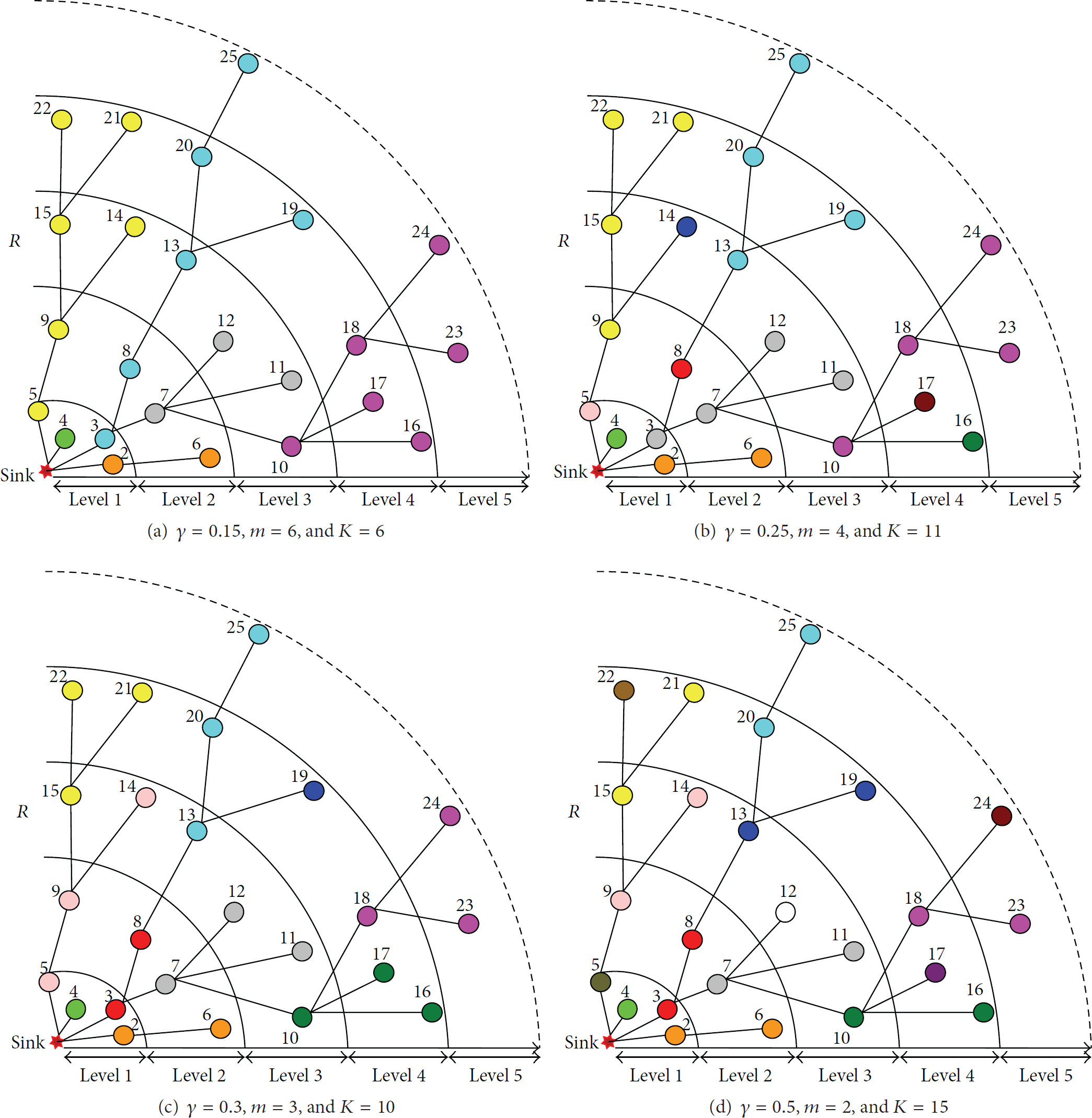
Figure 6 gives the node set T for each time-slot during which all the member nodes of T synchronously send packets to their corresponding parent nodes. For example, when $\gamma =0.15$ , a cycle time is composed of 18 time-slots in Figure 6(a). Node 3 is assigned three slots of 13, 17, and 18. Packets from nodes 3, 8, 13, 19, 20, and 25 can be aggregated into one data packet and transmitted to the sink in the time-slot 13. The final aggregated data of node 10 can be transmitted to the sink in the time-slot 17, and the aggregated data of node 7 can be transmitted to the sink in the time-slot 18.

Figure 6

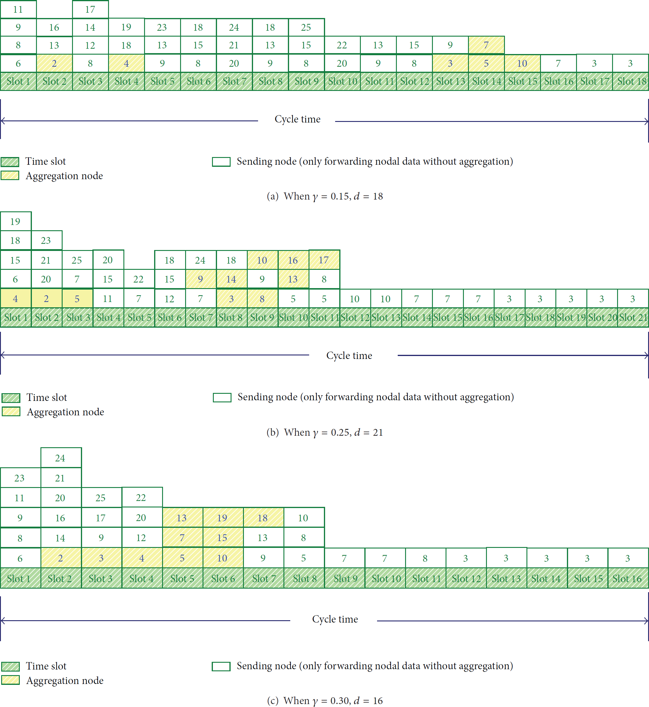
The node set T for each time-slot under different aggregate rates.

6. Performance Evaluation

In this section, compared with a non-round-up integer time-slot allocation approach named SDAS, the performance of the proposed MIDAS approach under different aggregation rates is evaluated. The aggregation rate of each sensor node is fixed to 0.15, 0.25, 0.3, and 0.5, respectively. The simulation is conducted on the platform of MATLAB 7.0 and the performance of the scheme is evaluated in a wireless sensor network with tree topology. And a child-parent relationship has been established. In each sample period, each node is sampled once and generates its original data packet synchronously at each sample initial time 0. The amount of information contained in an origin data packet is assumed to be 1 unit. And the number of aggregated data packets is calculated by (4). Table 3 shows the parameters and corresponding values in the network. Moreover, we assume the energy of sink is infinite and all the other nodes have the same initial energy 2 J. The energy cost only takes place in the case of receiving or transmitting data packet, which is calculated by (2) and (3). The energy utilization efficiency can be calculated by (11).

Table 3

Network parameters.

Symbol	Value	Symbol	Value
Initial energy $E_{\text{init}}/$ J	2	Packet size δ/bytes	5 ∗ 105
Threshold distance $d_{\mathrm{0}}$ /m	87	$e_{fs}/$ pJ⋅(b⋅m2)−1	10 $\text{pJ}$
Sensing range $r_s/$ m	10	$e_{\text{amp}}/$ pJ⋅(b⋅m4)−1	0.0013
$E_{\text{fusion}}$ /nJ⋅b−1	5	$E_{\text{elec}}/$ nJ⋅b−1	50

6.1. Node Scheduling Time-Slot Assignment

Figure 1 shows a randomly generated aggregation tree. Except the sink, distance from one node to its parent in the aggregation network is as shown in Table 4. Exploiting the proposed MIDAS, the result of node scheduling time-slot assignment of the aggregation tree shown in Figure 1 is presented in Table 5. The scheduling result is denoted by time-slots of each node to transmit. As can be seen in Table 5, each node has been assigned one slot or multislots. These time-slots of one node can be used for different purposes. For example, when the aggregation rate $\gamma =15\%$ , the first time-slot to transmit for node 7 is the 14th time-slot; node 7 is sampled and aggregates with incoming data packets from nodes 11 and 12, and then it transmits the aggregated packet to its parent directly in the 14th time-slot. The second time-slot to transmit for node 7 is the 16th time-slot. And node 7 transmits the aggregated data packet of node 10 to its parent directly in the 16th time-slot. Exploiting algorithm SDAS, the result of node scheduling time-slot assignment of Figure 1 is presented in Table 6.

Table 4

Parent-child relationships and distances from child to parent node in the aggregation tree of Figure 1.

Node ID	1	2	3	4	5	6	7	8	9	10	11	12	13
Parent ID	×	1	1	1	1	2	3	3	5	7	7	7	8
Distance (m)	×	91	95	56	96	82	55	64	77	98	98	58	99
Node ID	14	15	16	17	18	19	20	21	22	23	24	25	×
Parent ID	9	9	10	10	10	13	13	15	15	18	18	20	×
Distance (m)	98	74	90	57	71	96	90	98	83	52	92	97	×

Table 5

Node scheduling of MIDAS of Figure 1 under different aggregation rates.

ID	1	2	3	4	5	6	7	8	9	10	11	12	13
γ = 15%	×	2	13, 17, 18	4	14	1	14, 16	1, 3, 6, 9, 12	1, 5, 8, 11, 13	15	1	3	2, 5, 8, 11
γ = 25%	×	2	8, 17, 18, 19, 20, 21	1	3, 10, 11	1	3, 5, 7, 14, 15, 16	9, 11	7, 9	9, 12, 13	4	6	10
γ = 30%	×	2	3, 12, 13, 14, 15, 16	4	5, 8	1	5, 9, 10	1, 8, 11	1, 3, 7	6, 8	1	4	5, 7
γ = 50%	×	2	3, 18, 19, 20, 21, 22, 23, 24, 25	4	1, 5, 9, 10	1	5, 9, 14, 15, 16, 17	1, 7, 10	3, 7, 8	6, 11, 12, 13	1	7	5, 8
ID	14	15	16	17	18	19	20	21	22	23	24	25	×
γ = 15%	3	6, 9, 12	2	3	4, 6, 8	4	7, 10	7	10	5	7	9	×
γ = 25%	8	1, 4, 6	10	11	1, 6, 8	1	2, 4	2	5	2	7	3	×
γ = 30%	2	6	2	3	7	6	2, 4	2	4	1	2	3	×
γ = 50%	2	4, 6	2	7	8, 10	2	6	1	5	1	9	1	×

Table 6

Node scheduling of SDAS of Figure 1 under different aggregation rates.

ID	1	2	3	4	5	6	7	8	9	10	11	12	13
γ = 15%	×	2	4, 13, 14, 15, 16, 17, 18, 19	1	3, 8, 9, 10	1	3, 6, 10, 11	7, 9, 12	4, 6, 7	7, 9	5	1	3, 8
γ = 25%	×	2	4, 13, 14, 15, 16, 17, 18, 19	1	3, 8, 9, 10	1	3, 6, 10, 11	7, 9, 12	4, 6, 7	7, 9	5	1	3, 8
γ = 30%	×	2	4, 13, 14, 15, 16, 17, 18, 19	1	3, 8, 9, 10	1	3, 6, 10, 11	7, 9, 12	4, 6, 7	7, 9	5	1	3, 8
γ = 50%	×	2	4, 17, 18, 19, 20, 21, 22, 23, 24, 25	1	3, 8, 9, 10	1	3, 6, 13, 14, 15, 16	7, 9, 12	4, 6, 7	7, 10, 11, 12	5	1	3, 8
ID	14	15	16	17	18	19	20	21	22	23	24	25	×
γ = 15%	1	2, 5	1	2	8	1	6	1	3	1	3	1	×
γ = 25%	1	2, 5	1	2	8	1	6	1	3	1	3	1	×
γ = 30%	1	2, 5	1	2	8	1	6	1	3	1	3	1	×
γ = 50%	1	2, 5	1	2	8, 9	1	6	1	3	1	3	1	×

6.2. Energy Utilization Efficiency

We compare the energy utilization efficiency property of the proposed MIDAS approach with that of SDAS.

First, based on the result of node scheduling time-slot assignment presented in Section 6.1, we could obtain the residual energy of each node in network of Figure 1 when the network dies, which is shown in Figures 7 and 8, respectively.

Figure 7

The residual energy of the MIDAS of Figure 1.

Figure 8

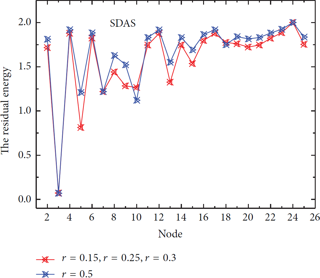
The residual energy of the SDAS of Figure 1.

Also, we consider the case when the number of nodes in the network is increased to 100 randomly. The network parameters and aggregation scheduling algorithm are the same as the ones above. Figures 9 and 10 show the residual energy of each node by running the two algorithms, respectively.

Figure 9

The residual energy of the MIDAS with 100 nodes.

Figure 10

The residual energy of the SDAS with 100 nodes.

We can see that there is an obvious fluctuation characteristic in Figures 7 and 9. The nodes that consume more energy are not always in hotspot when the network dies. Energy dissipation is larger for most sensors in the middle layer of network, during the entire execution of the data transmission. For example, node 10 and node 13 in Figure 7 consume more energy. But in Figures 8 and 10, it can be seen that when the network dies, the nodes which consume more energy are always in the area near the sink under no matter what aggregation rate. This means that the energy consumption is larger in the area near the sink but is smaller in the area far from the sink. From Figures 7–10, we can see that our MIDAS approach can make full use of the remaining energy of peripheral nodes than SDAS.

Second, we compare the energy utilization efficiency of our MIDAS approach with that of SDAS under the different aggregation rates and different network scales. Simulations are conducted on the network with nodes of 25, 50, 75, and 100, respectively. The results are shown in Figures 11, 12, 13, and 14, respectively.

Figure 11

The comparison of the energy utilization efficiency under 0.15 aggregation rate.

Figure 12

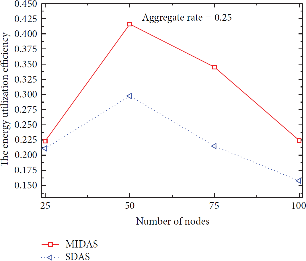
The comparison of the energy utilization efficiency under 0.25 aggregation rate.

Figure 13

The comparison of the energy utilization efficiency under 0.3 aggregation rate.

Figure 14

The comparison of the energy utilization efficiency under 0.5 aggregation rate.

Figures 11, 12, 13, and 14 compare the energy utilization efficiency of the network by using the two algorithms when the number of nodes varies. It can be seen from the figure that the energy utilization efficiency of the proposed MIDAS approach outperforms that of SDAS significantly. The energy utilization efficiency of MIDAS algorithm is mostly about 25%–45%, but that of SDAS algorithm is mostly about 15%–25%. The energy utilization efficiency of MIDAS algorithm is improved by 30% compared with the SDAS algorithm. This is because some nodes in the middle layer consume more energy for transmitting more data packets. Thus the residual energy of these nodes decreases when the transmission data packets increase. Therefore, the remaining energy far away from the sink is fully utilized, which increases the energy utilization efficiency of the network.

From Figures 7–14, we can see that our MIDAS approach can make full use of the remaining energy of peripheral nodes than SDAS so that performance of our method is better than that of SDAS in the energy utilization efficiency.

6.3. Network Lifetime

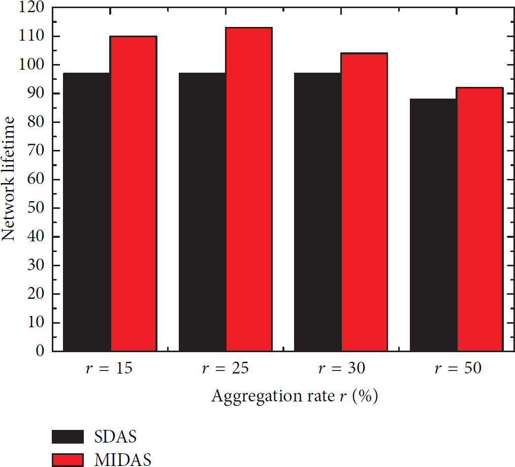
The network lifetime is an important metric to evaluate our approach. We compare the network lifetime of the proposed MIDAS approach with that of SDAS under the different aggregation rates and different network scales. Figures 15, 16, 17, and 18 show the comparison of network lifetime under the two scheduling approaches, respectively.

Figure 15

The comparison of the network lifetime with 25 nodes.

Figure 16

The comparison of the network lifetime with 50 nodes.

Figure 17

The comparison of the network lifetime with 75 nodes.

Figure 18

The comparison of the network lifetime with 100 nodes.

From Figures 15–18, we can see that the proposed MIDAS approach has a better performance in the aspect of network lifetime. The network lifetime of MIDAS is improved by 20% compared with that of SDAS under the same aggregation rate and the same network scales. This is because the proposed MIDAS approach has the ability to reduce the number of receiving and sending data packets near the sink for decreasing the energy consumption in this area by selecting reasonable nodes to aggregate. The aggregation nodes hold on transmission and accumulate their data before sending them to sink at once. Consequently, the energy consumption is reduced because the data needed to be scheduled in the network is reduced. This property is important since it prolongs the network lifetime by avoiding early energy depletion of sensors. Moreover, the improvement of network lifetime will be larger with the increase of the aggregation rate. This is because the number of data packets gathered by the sink decreases when the aggregation rate of nodes increases.

7. Conclusion

This paper focuses on the data aggregation scheduling combining time-slot and variable aggregation rate. Based on the aggregation model and the given aggregation rates, we proposed an efficient aggregation approach, which includes two coupled parts: aggregation set construction and an aggregation scheduling algorithm. The proposed approach can not only minimize the number of receiving and sending data packets in hotspot but also reduce the number of aggregated packets in network for better scheduling performance in network lifetime. Furthermore, it is also essential to increase energy utilization efficiency of the nodes in the middle layer by exploiting the remaining energy of peripheral nodes. Our simulation results verify the effectiveness of the MIDAS scheme. The dual goals of improving the network lifetime and increasing the energy utilization efficiency are simultaneously achieved.

In this paper, we focus on the fact that data aggregation rate is equal for every node. It would be interesting to study the algorithm extending to the case that nodes may have different data aggregation rates.