
Abstract
In wireless sensor networks energy is a very important issue because these networks consist of lowpower sensor nodes. This paper proposes a new protocol to reach energy efficiency. The protocol has a different priority in energy efficiency as reducing energy consumption in nodes, prolonging lifetime of the whole network, increasing system reliability, increasing the load balance of the network, and reducing packet delays in the network. In the new protocol is proposed an intelligent routing protocol algorithm. It is based on reinforcement learning techniques. In the first step of the protocol, a new clustering method is applied to the network and the network is established using a connected graph. Then data is transmitted using the Q-value parameter of reinforcement learning technique. The simulation results show that our protocol has improvement in different parameters such as network lifetime, packet delivery, packet delay, and network balance.
1. Introduction
Energy is a significant factor in the wireless sensor networks (WSNs) [1]. Therefore, most researchers are concerned with routing protocols and the energy efficiency factor. Initially, more attention in current protocols was on Quality of Service (QoS), bandwidth, packet delivery, and reliability factors and attention to the energy issue was less [2]. The researchers gradually focused on the energy factor when they understood that energy is an important parameter in the WSNs. The sensor nodes are small-size devices that have very low batteries and their charging is impossible in most applications [2]. Therefore, the engineers found that energy-saving is a very important issue in most applications, although energy-saving has tradeoff with some of the design factors such as reliability or system overhead. Therefore, they should create a balance between the design factors [3]. The hierarchical routing protocols have a good performance among the routing methods on the issue of energy efficiency. We know that cluster-based protocols may be appropriate for some applications. In fact, the network protocols are depended to special applications. If the algorithms have integrity and ability, then techniques are generalizable to more applications. Energy efficiency schemas are methods for energy-saving and prolonging network lifetime. These approaches are different in the WSNs from duty cycle or data-driven methods [4]. The new protocol uses data aggregation and learning-based methods which are a subset of the data-driven category.
The hierarchically based protocols are suited to the energy-saving issue. In these protocols, networks are divided into clusters and have a CH node for each cluster [5]. The CH nodes are intermediaries between the sensors in their cluster and other clusters or BS/sink. There are different clustering models in the researches. For example, in some of the protocols CH nodes are selected for each cluster and then the nodes decide which ones can be members of that cluster. This decision can be based on different parameters such as residual energy, distance to other nodes, and distance to BS/sink. In some others, in the beginning each node knows to which cluster it belongs and then selects a CH node for that cluster [5]. Our protocol is based on the second category, so the nodes are placed in a cluster and then select a CH node to their cluster. In this protocol, the main aim is selection of optimal CH node. Selection of CH nodes imposes overhead control on the network. This issue is not considered in many hierarchically-based protocols. Therefore, we propose a new routing protocol for our network.
As mentioned before, absolute energy-saving has trade with some parameters such as reliability and system overhead. The new protocol creates a balance between them and therefore we do not consider energy efficiency absolutely. This does not mean that we give no attention to the energy issue and our main goal is still energy efficiency.
On the other hand, the new protocol has fault tolerance ability, so failure of a path does not cause loss of the data packet. Therefore, this approach is reliable and fault tolerant. Fault management is not considered in many protocols [6]. In these protocols, when failure occurs in the network, the nodes send special data packets to fix the problem but it would cause significant overhead in the system that could lead to increased latency and packet loss of real data packets in the network [6]. Also, the preference of some others is retransmission. The proposed protocol in this paper solves these problems.
The routing phase in the new protocol is a novel approach. The network was run in periodical times called rounds. In each round, the CH nodes are changed and hence the tree structures are reorganized. The modifications cause overhead on the whole network. In this paper, we propose a routing algorithm based on an intelligent approach, so that the learning and routing phases are realized at the same time. This strategy avoids wasting energy in the learning phase and reduces the overhead of the system. This phase will be described in the next sections as well as the other phases of the protocol. We will describe the operation of the proposed protocol and then explain it with the help of the pseudo code and flow chart methods. Thereinafter, simulation of the protocol is done and the results are shown in graph charts. Finally, we will compare it with some of the current protocols such as LEACH [7], HEED-NPF [8] and EECS [9].
2. FTIEE Algorithm Description
Clustering is a process in the WSNs in which the network is divided into several clusters. Each cluster has a CH node which sends collected data from the nodes of its group to BS/sink. As mentioned above, selection of the CH node is an important issue in the hierarchical based protocols and it increases the overhead of the system. If the CH node crashes then this will generate considerable overhead in the network.
Our goal is to propose an energy efficiency protocol that reduces system overhead and increases reliability as much as possible. In this protocol, all nodes within a cluster can be a CH node and clusters do not have to have a CH node and this election is done by means of learning machine. In fact, we want to increase network lifetime by reducing energy consumption, where the energy is wasted in repeated elections of CH nodes. All processes of the protocol will be described in the next section.
The learning machine techniques are categorized into several methods such as reinforcement learning approach [10] and genetic algorithms [11]. Reinforcement learning is studying computer algorithms that the routes are optimized by their own experiences automatically [10]. The basic issue in the reinforcement learning is learning an agent by the self-environment method. In most methods, learning actions is done in periodic times and selection of an action is based on a special policy at that moment. The agent receives a reward value for every act of selection. The goal of algorithms is maximizing the values for faster learning. FTIEE uses the reinforcement learning approach to data routing. Some of the terms are from reinforcement techniques such as action, agent, state, reward, episode, and policy. Agent is a learner that optimizes its behavior over the learning process time. Action is a series of activities that an agent can do. Reward is a value that an agent receives from the environment for every action and it can be positive or negative. State shows the mode of the agent. Episode is a set of states that an agent passes to reach the goal. Policy is concerned with choice of an action by the Agent. Policies are defined in the different models as greedy and ε-greedy policies [12]. The greedy policies choose the best action at the moment. They are not good policy because they may fall into traps. ε-greedy policies are similar to greedy approaches but they choose the best action with a small epsilon possibility. In this case does not cause the algorithm to fall into traps or does not reach local optimal answers. A WSN is based on reinforcement learning with multiple agents. In the networks, agent is a sensor node, action is the next hop of each node, and the agent state is the routing cost of a node to BS/sink via their neighbors. Indeed, it indicates a multi-hopping communication system that is more common in hierarchical-based protocols. A success and energy efficient data transfer of data in the algorithm gives a positive reward to a node; otherwise, it gives a negative reward. These rewards help find correct (energy efficient or reliable) routes to any node.
FTIEE is based on the hierarchical-based protocol. Numbers of clusters are constant but, unlike it, the shapes of clusters are square. The size of clusters is variable in FTIEE and it is based on a rule. Clusters that are close to BS/sink are smaller than clusters that are located towards the BS/sink. In fact, the size of the clusters increases with increasing distance to the BS/sink. This is a method where the clusters initially form and then a CH node is selected for them.
The nodes work together for data transmission to the BS/sink; thus, the nodes that are closer to the BS/sink will consume more energy than the other nodes. Therefore, it is possible that the clusters close to the BS/sink may convert to nonconnect status. Hence the sensed data does not reach the BS/sink. To solve this problem, the clusters near the BS/sink have smaller sizes. Therefore, some energy will be saved for data transmission. Figure 1 represents an example about clusters and their sizes.

Size of clusters in FTIEE protocol.
We use some parameters as coordinates of the BS/sink, the maximum and minimum size of the clusters and the growth rate of clusters in different sizes. The sensors must use their cluster-ID for intra-cluster coordination. For this purpose, the network is divided into clusters with a maximum size and then a unique identify number is assigned to each of the clusters. The ID-numbers will be used in routing and CH node selection. For example, if the network deployment area is 2000*2000 and the maximum cluster size is 500*500 then the network will be divided into 16 clusters and their ID will be from 1 to 16 according with Table 1.
Assignation of ID number to each cluster.
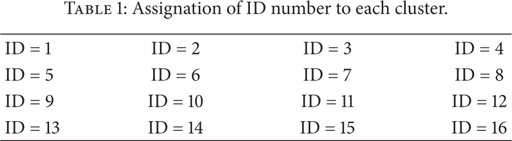
Firstly, we divide the network into several clusters with maximum sizes and then calculate the size of the cluster in which BS is placed. In this case, it will be divided into the minimum possible size. After this, the size of the adjacent clusters is calculated by following this formula (Algorithm 1).
Grow-rate = Main cluster that BS is within it and Min-size = Max-size * (1/Grow-rate) Grow-rate = 1 Adjacent cluster size = Min size * (Grow-rate + 1) Other cluster size = Max-size if Adjacent cluster size ≥ Max size Grow-rate = Main cluster that BS is within it and Min-size = Max-size * (1/Grow-rate) Adjacent cluster size = Min size * [ Other cluster size = Max-size if grow-rate value is 1 for next step
If the growth rate is very small, then the clusters will grow slowly. The value of the grow rate parameter will be updated with each movement away from the BS/sink. Figure 1 indicates one division of the network into different clusters with different size. In Figure 1, the maximum size is 500 and the minimum size is 125 and the growth rate is 2. It should be noted that if the value of growth rate is one, then the size of the clusters will be the same.
The stability of the clusters is another important issue in hierarchical-based protocols. In some of the current approaches, the number of clusters is less over the passage of time, but the number of clusters in our approach is always stable and fixed. One other point is that CH nodes have multi-hop communications to the BS/sink. It should be noted that some of the protocols do not focus on this case and they use direct link between CH nodes and the BS/sink. The next issue in FTIEE protocol is connectivity. It is based on full connectivity and graph theory.
In our protocol, sensor nodes do not need to identify the CH node. A sensor node sends its data to the BS/sink using its cluster-ID and basic information about its neighbors that have one hop distance from it. Our protocol is a distributed and local approach that finds the optimal CH nodes of each cluster by the learning system. In this case, each node can be a CH node or selects the best path to data transmission. Therefore, the algorithm has a good flexibility rate, so that the sensor nodes are not involved in CH election and therefore, energy consumption and system overhead is reduced. The main criterion in CH node selection is dependent on the current state of the nodes and their neighbors. FFIEE uses a reinforcement learning approach that is called the Q-learning technique [12]. This algorithm is able to learn the optimal CH node and manage some problems such as node failure. The optimal CH node is a node which has the shortest cost to the BS/sink. Each of the sensor nodes is an independent learning agent and chooses its actions for data transmission to a neighbor or selects himself as CH node. As mentioned above, an action is the next hop of a node. If the next hop is its own node, then it will buffer received packets for determined period of time and send them to the BS/sink. The reward system in our protocol is indicated by a Q-value variable [12]. It is calculated by two parameters. The first is based on a value that is dependent on distance between a node and the BS/sink. It is suitable to reduce overhead. The second is based on the residual energy of a node. It is appropriate for delay control in the whole network. Indeed, these parameters are cost functions of FFIEE protocol. In summary, the main Q-value is the multiplication of the Q-value of a node and the Q-value of its actions. This is shown in Figure 2, for better understanding of this issue. The value is changed by the actions selection of the agents and it is calculated by the formula bellow.


A general view of Q-values calculation.
R is a reward value and α is the learning rate. If the value of α is one, then the learning rate will increase and the formula will change to the following mode. In fact, the reward value determines the action of a node to find optimal route to send data to the BS/sink. The policy of actions selection is based on ε-greedy approach. Consider

The pseudocodes of A and B parts of Q-value calculation are represented in Listings 1 and 2. The algorithm computes the value of each node (A part) using the distance between nodes and the BS/sink. The values of the nodes that are farthest relative to the BS/sink are lower than those of near nodes. The algorithm computes the value of each action (B part) by considering the battery level in each node. So, if the battery is high, then the calculated A value will have more impact, intervening in the main Q-value and will reach reduce packet delay in the network. Otherwise, the B value will have more impact, intervening in the main Q-value and will balance energy consumption in the whole network.
// // n: number of nodes // // (1) Cost of BS = n (2) For each neighbors of BS, for example BS sends (3) Each neighbor such as K receives node K send (4) Repeat Step 3 even all nodes receive
// computing Q-value of each action // we define a possible action as with i // N: number of neighbors of node i // Q( // // if ( Q( else Q(
In general, our protocol learns finding optimal CH nodes and paths at the moment of network rounds. In other words, when the optimal CH nodes are learned, paths within a cluster will be learned automatically. Therefore, finding paths in our protocol does not have extra overhead over the system. Figure 5 represents learning model in finding optimal CH nodes and paths in the network. As previously mentioned, the topology of the network is based on connected graphs. In the FTIEE, data transferring and routes detection are parallel and on-demand. This technique is one of the special properties of the FTIEE.
In Figure 3, all nodes will send their data to the node that has more Q-value. In other words, the nodes will learn by repetition of the learning process. The CH node can change over time due to updating Q-values. We have two problematic issues in this case of our algorithm. Our graph may be nonconnected in the network or any cluster. In this case, the algorithm can identify the two CH node for each nonconnected parts automatically. This concept is illustrated in Figure 4.

Communications form a connected cluster sample (a) before running and (b) after running the algorithm.

Communications form a nonconnected cluster sample (a) before running and (b) after running the algorithm.

An example of fault tolerance in FTIEE protocol.
As was explained above, in our protocol the routing phase is based on an intelligent approach so does not need CH election in all rounds because it can select optimal CH nodes at different periodic times of the network rounds by the learning mechanism. It does not have one CH node at each cluster and the number of CH node could be more. If there is much learning time, then the algorithm operates well. It is significant to note that this algorithm has a parallel schema in finding optimal paths and transferring data. This is an ability which due to increasing performance in intelligent based approaches. In general, priority data transferring in FTIEE is as follows.
Data is sent to a node that has more Q-value. If the Q-value of two nodes is same, then data will be sent to one of them randomly even if the node is within another cluster. Meanwhile, the order of maximum Q-value is chosen by ε-greedy approach. This does not cause it to fall into traps or the local optimal solutions.
The concept of effective energy is observed in the protocol too. It saves energy by only using a data-driven schema. In fact, FTIEE uses the learning-based and data aggregation methods [4] to energy consuming management. The protocol does not use the sleep/wakeup method to energy-saving in the network. It should be noted that the management of a shared channel is realized by the TDMA approach [13].
Reliability and fault tolerance ability is one of the strengths of the protocol. This will cause increasing packet delivery and reduction of packet loss. Also, the network is connected for a long time because it finds new routes in deterioration of the paths or node failure. In Figure 5, node B is in failure and node A cannot send data to node C. This is a serious problem. In our protocol, the node A waits for a short time and then selects itself as CH node. During the waiting period, it aggregates received data from other nodes and then sends them to the BS/sink using its other neighbors from the close cluster.
When the network is passive or idle, our approach to learning does not consume energy. It saves energy in the network as a whole. It should be pointed out that the learning part of the routing protocol is done on active sections because the learning phase is parallel to routes detection. As mentioned above, the available parameters to routing in FTIEE are the Q-values, the batteries of each node and ID-cluster. Generally, FTIEE focuses on three important parameters which are network lifetime, packet delay and delivery. It seems that FTIEE has acceptable performance for some applications. It will describe in the next sections. Also, the FTIEE algorithm is represented by a flow chart in Figure 6 and pseudocode in Listing 3.
(1) Each node sends a message to all its neighbors to receive their costs. When a node runs out of energy, (2) When a node such as K wants to send a packet it chooses the next node as described below: (2.1) for all neighbors of the same Id with its Id: (2.1.1) if (cost of neighbor > its cost) (i) Then compute Q-value of it. (ii) Sends the packet to the neighbor with the highest Q-value. (iii) if some of neighbors have same Q-value, chose one of them randomly. (2.1.2) else if (any neighbors has not the same Id with its Id OR cost of neighbors with the same Id <= its Id) Go to Step 2.2. (2.2) for all neighbors in adjacent clusters: (2.2.1) if (cost of neighbor > its cost) (i) Compute Q-value of it. (ii) Sends the packet to the neighbor with the highest Q-value. (iii) if some of neighbors have same Q-value, chose one of them randomly. (2.2.2) else chose one of neighbors randomly. // in this case the node K is cluster head

General views of FTIEE protocol.
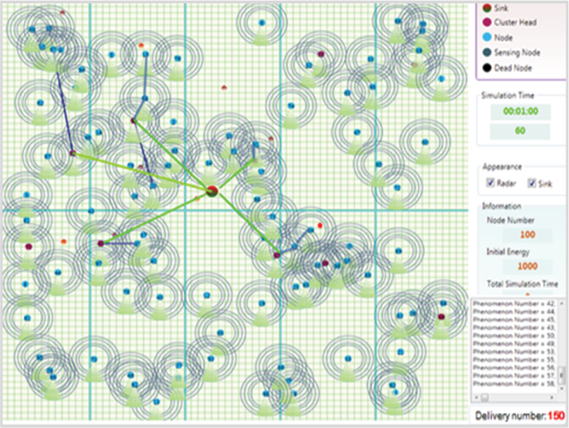
Figure 7 represents a snapshot of new protocol in during the simulation. In fact, the routing and data transferring approach is based on intelligent routing. As mentioned before, new protocol could have several CH nodes in each cluster. Also, it is reliable against faults. Figure 7 represents an example state of the FTIEE operation. In this case is supposed that the protocol has 100 nodes, one phenomenon per second and ten clusters initially. In the paper, new protocol is simulated and is compared with some current protocols as HEED-NPF [8] and EECS [9]. All conditions are the same for FTIEE and HEED-NPF, EECS. All snapshots are one-minute of running of the network. Figures 8 and 9 are a snapshot of another protocols. All three snapshots have been taken in the same conditions of initial energy, node numbers, interval, and duration of the phenomenon. They will be explained in detail in the simulation section.

A snapshot of basic network topology in FTIEE protocol.
A snapshot of basic network topology in HEED-NPF protocol.

A snapshot of basic network topology in EECS protocol.
We will explain the FTIEE simulation section by its gained results from the simulator tool. The other protocols as HEED-NPF, LEACH, and EECS will be evaluated and will be compared with our protocol results. We are using the same conditions to increase the precision and validity of the simulation results.
3. Simulation
We have developed a WSN simulation tool in the C# program so it is based on NS-2. The tool is applied to four protocols under the same conditions in this paper. It allows having results documentation or simulation charts in the network lifetime, packet delivery and packet delay parameters at the moment or at the end. In this case study, output parameters are network lifetime, packet delivery, packet delay, and network balance. Also, we use the original simulation charts and parameters of HEED-NPF, LEACH and EECS to demonstrate the correctness of our protocol. The input parameters are the initial energy of each sensor nodes, energy consumption rate, transmit, receive, and sense process costs, and send/receive buffer size. All four protocols are performed in parallel and have the same values for the parameters. Therefore, the simulation results will have a high degree of confidence.
The tool uses the same nodes count and location of sink to increase the accuracy of the simulations. Table 2 shows an example of input parameters values which are constant and the same for all protocols in a simulation. It should be noted that the values have been used as several examples of protocols, and we can use arbitrary values for simulations. In this case, we suppose that information about of sensor location is available; therefore, we do not consider location of nodes and time synchronization [14] in the four protocols. Also, the current protocols did not consider these issues. In this case study, the number of clusters in cluster-based approaches is constant and its value is 10. It should be noted that clusters are resized in FTIEE and thus the number of clusters can increase. We consider that the input parameters are the same in the four algorithms. The first simulation applies Table 2 to illustrate comparison results of the network lifetime, packet delivery and packet delay. Deployment of sensor nodes is random and the nodes are distributed in a two-dimensional space. The BS/sink can be in any arbitrary position, inter or out of the network and does not have a limitation battery or computing power. Locations of nodes and sink are fixed after their establishment.
Values of input parameters for FTIEE protocol.

We can say that increasing number of nodes increase number of received packets but packet delivery rate is almost reduced because some factors such as increasing density of nodes, hop count and node failure probability are affective. Also, an increasing number of nodes increase the network lifetime and packet delays.
We illustrate the performance of FTIEE in 4 models. In fact, these models are output parameters of the simulation tool. They are network lifetime, packet delivery, pocket lost, and network balance. Figure 10 shows a case of network lifetime using 100, 200, 300 and 400 nodes. The network is active up to the death of the last sensor. In some of the literature, the network is alive as long as there is at least one connection between sensor node and sink. The assumption of our simulation tool is the first case. It should be noted that the input parameters in simulation processes are based on values of Table 2.

The network lifetimes in FTIEE protocol with 100, 200, 300, and 400 nodes.
We illustrate delivery and loss packets performance in the FTIEE with the same values in Figures 11 and 12. The packet delivery has two means in the literature. The number of packets successfully transmitted from node to sink is one of the means. Second means is total packet received from the sink. We sum the two values to find the packet delivery value. Packet loss is gained from subtraction of all sensed data packets and the number of delivered packets. In this paper, our protocol focuses on the factors of packet delivery, reliability and network lifetime. It tries to create a balance between the parameters. It is relatively good compared to the other (same) protocols because it has a good lifetime, packet delivery rate and network balance. In fact, it is an appropriate energy efficient approach. Figure 11 illustrates the packet delivery rate of FTIEE using different numbers of nodes. Figure 12 shows the numbers of packets lost in the network when FTIEE works with 100, 200, 300, and 400 sensor nodes.

Number of delivered packets in FTIEE protocol with 100, 200, 300, and 400 nodes.
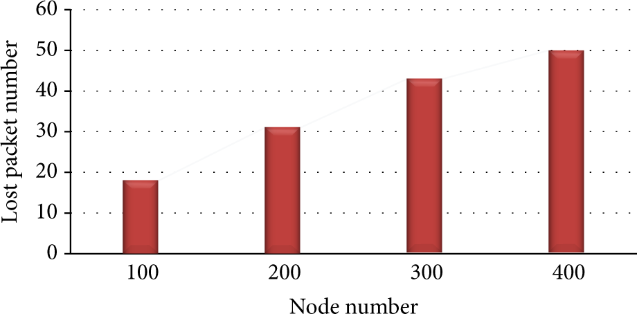
Number of lost packets in FTIEE protocol with 100, 200, 300, and 400.
Figure 13 explains the relation between lost and delivery packets in our protocol. Appropriate rates in the lost packets and delivery packets cause increasing system reliability and fault tolerance. When a node on path is dead, our algorithm selects the previous node and introduces it as CH node. Also, it can use the other nodes that are members of the adjacent cluster. Packet delivery rate rises with the increasing number of nodes in our simulation area. This issue has direct relation to the low rate of lost packets.

Relationship between lost and delivered packets in FTIEE protocol with 100, 200, 300, and 400 nodes.
Also, Figure 14 presents the relation between network lifetime and packet delivery with 100 nodes. As time progresses, the nodes begin to die or fail, therefore the packet delivery rate will decrease. We assumed new node cannot be added to the network.

Relationship between delivered packets and network lifetime in FTIEE protocol with 100 nodes.
Network balance is another measure of simulation in our protocol. Some of the output parameters have trade-off. An example is as follows: if the main goal of the network design is increasing reliability rate, the network lifetime will automatically reduce. With this description, if a protocol can create a balance between output parameters, it will have a good performance. It can gain from different methods, such as, percentage of packets delay to network lifetime (Figure 15).

An example view from network balance rate in FTIEE protocol.
It seems the great advantage of our protocol is balance in the whole network. Packet delay can be high in the protocol because the algorithm selects alternative paths for successful transmission. The alternative routes create delay in the networks. However, the algorithm has good performance in packet delivery rates, so it may be suitable in data-oriented applications or real-time systems. In the next section, we will compare our protocol with LEACH, HEED-NPF, and EECS protocols.
4. Comparison and Results
As mentioned before, we have developed a WSN simulation tool in the C# program and use it for all simulations in our paper. In this section, the tool is applied to four protocols (LEACH [7], HEED-NPF [8], EECS [9], and FTIEE) in the same conditions and input parameters. The tool allows us to have results in the network lifetime, packet delivery, and energy consumption parameters at the moment or end as charts. In this case study, output parameters are the network lifetime, packet delivery, energy consumption, and network balance. We use the original simulation values of LEACH, HEED-NPF, and EECS to demonstrate the correctness of our protocol results. The input parameters are the initial energy of sensor nodes, radio and sensor energy consumption, the transmission and sense process cost, and send/receive buffer size. All protocols are performed in parallel with the same values for the parameters. Therefore, the simulation results will have a high degree of confidence.
We use the main results simulation of each of the current protocols, so that they can be compared with our protocol. For this, we must use similar input parameters with them. The gain results illustrate that our protocol have greater optimizing than LEACH, HEED-NPF, and EECS. These protocols have different values of the input parameters. Hence we simulate our protocol separately with each of the protocols with the same values.
As mentioned before, an increasing number of nodes increase number of received packets but packet delivery rate is almost reduced because some factors such as increasing density of nodes, hop count, and node failure probability are affective. Also, increasing number of nodes increase the network lifetime and packet delays. Firstly, we simulate FTIEE with the values of input parameters which are based on Table 3 and then compare with EECS and LEACH. The number of clusters is 10. We simulate our protocol and the two protocols parallel to our tool and evaluate their results in graphic charts. In this case, simulation is done on the first, half and last nodes to die. Figures 16, 17 and 18 present the results with 400, 600, and 1000 nodes. In [9], EECS is compared with LEACH therefore, we use from the results of both in our simulations. In continuously, we simulate four protocols and show the results in the simulation charts.
Values of input parameters in original reference of EECS protocol [9].


The first node time of death in LEACH, EECS, and FTIEE with 400, 600, and 1000 nodes.

The half node time of death in LEACH, EECS, and FTIEE with 400, 600, and 1000 nodes.

The last node time of death in LEACH, EECS, and FTIEE with 400, 600, and 1000 nodes.
In this section, all protocols are simulate using new simulation tool, so we will apply various different parameters and analyze the performance of each protocol. We assume that the values of the input parameters are as listed in Table 4. We run each of the protocols in seven cases with different node numbers. In another part of the simulation process, we will present offline running of our algorithm with the same input parameter values to the increasing learning rate and find the optimizing factor. The offline running would give more desirable results. The HEED-NPF is similar to our protocol partly because it uses an expert approach in the routing process [8]. As it seems, FTIEE has a good performance in the network lifetime and can increase this factor by data aggregation and new intelligent approach. As mentioned before, our intelligent algorithm uses different mechanism in CH node election and routing. FTIEE finds routes when it needs to send data. This method is somewhat similar to the HEED-NPF method. Figure 19 illustrates results of all four protocols in terms of network lifetime. Our protocol has better performance than other protocols and its improvement is about 2.5% higher than HEED-NPF, 6.5% higher than EECS, and 16% higher than LEACH.
Values of input parameters in four protocols.


Simulation results based on network lifetime parameter in different node numbers cases for FTIEE, EECS, LEACH and HEED-NPF protocols.
The second case for comparison is packet delivery. New protocol has a more acceptable optimization performance in the packet delivery than LEACH, HEED-NPF, and EECS. The improvement is about 4.5% higher than HEED-NPF, 5.5% higher than EECS, and 44% higher than LEACH. Figure 20 shows the simulation results of the four protocols under the same conditions.

Simulation results based on packet delivery parameter in different node numbers for FTIEE, EECS, LEACH, and HEED-NPF protocols.
On the other hand, we simulate our protocol in the simulation area after 100 rounds of offline running. It should be noted that HEED-NPF ran with the same number of rounds in offline mode. The results show that our protocol is better than HEED-NPF. Indeed its growth rate is good. Based on the results, FTIEE improvement in the packet delivery factor is about 5.5% higher than HEED-NPF, 9% higher than EECS, and 47% higher than LEACH. Also, its improvement in network lifetime factor is about 4% higher than HEED-NPF, 9.5% higher than EECS, and 20.5% higher than LEACH.
The last simulation parameter is network balance. As mentioned before, network balance is another measure to simulate four protocols. If the main goal of network design is increasing reliability, then the network lifetime will automatically reduce. Indeed, if a protocol can create a balance between output parameters, then it will have a good performance in general. Figure 21 shows a case of network balancing comparison calculated on the relation between the number of delivered packets and the network lifetime.

A specific view from performance of LEACH, HEED-NPF, EECS, and FTIEE in network balance.
Briefly, the main goal of our protocol is energy-saving and increasing packet delivery while it maintains network balance. All goals are available simultaneously and are dependent on the usage environment. Hence, the algorithm can focus more on one of the parameters. For example, the lifetime parameter has greater priority than other output factors when energy-saving is an important aim in our application. In fact, this protocol is a general algorithm for different applications in the WSNs. However, the protocol has some shortcoming such as the need for offline working to reach a good performance.
5. Future Work and Conclusion
Unlike other networks, WSNs are designed for specific applications so characteristics and requirements are different in each of them. Therefore, they need new communication protocols, algorithms and designs. Moreover, factors related to network design must also be considered in order to achieve the expected performance in the WSNs. The most important constraint in the WSN is energy. Hence, it must be managed by techniques like algorithms. In the paper, we focused on the energy problem and proposed an algorithmic approach to have an energy-efficient and longer life network. Most researches in recent years are done related to energy-efficient wireless sensor network and one of the strategies is using a communication protocol based on clustering. The protocols have a CH node to create a connection between the nodes and the BS/sink. The selected CH nodes have control overhead in the network. Sometimes there is too much overhead. In this paper, we proposed a new routing algorithm for energy management and increasing network performance by using an intelligent algorithm. It manages the system overhead by means of CH selection. In the proposed method, all the sensor nodes can be CH node. They are chosen by a machine learning technique. This method saves energy in the whole network. The most important feature of the algorithm is routing mechanism and the paths detection.
Another important feature of FTIEE was fault tolerance. At first, when a failure occurred in the network, our protocol preferred to retransmit the packet instead of repairing or preventing faults. Retransmission has an overhead over the system but is better than other current protocols. Most other protocols send special data packets to repair faults.
Reliability and fault tolerance were some of the strengths of the protocol. There can cause packet delivery rate to increase and reduce packet loss. Also, the network can be connected for a long time because it finds new routes in case of deterioration of the path or node failure.
The concept of effective energy is observed in the protocol too. It saves energy by only using data-driven schema. FTIEE uses the learning-based and data aggregation methods. The methods are a subset of data-driven schema. The protocol does not use the sleep/wake up method of energy-saving in the network. It should be noted that shared channel management is realized by the TDMA approach.
According to the simulation results, our protocol had a good performance in delivered and lost packet numbers and network lifetime. Our output parameters were network lifetime, packet delivery and lost rate, the first, half and last node death time and the energy consumption rate. We simulated our protocol using the concurrent and offline running methods. FTIEE had a better performance in the offline method. Based on the results, FTIEE improvement in the packet delivery factor was about 5.5% higher than HEED-NPF, 9% higher than EECS and 47% higher than LEACH. Also, its improvement in the network lifetime factor was about 4% higher than HEED-NPF, 9.5% higher than EECS and 20.5% higher than LEACH. In the concurrent simulation method its performance in the delivered packet rate was about 4.5% higher than HEED-NPF, 5.5% higher than EECS and 44% higher than LEACH. Also, FTIEE improvement in the network lifetime was about 2.5% higher than HEED-NPF, 6.5% higher than EECS, and 16% higher than LEACH. Using fuzzy logic or Bayesian network on proposed protocol instead of machine learning approaches can be good. Also, agent based systems can help to learning process. The intelligent routing techniques like FTIEE and its combining with dynamic clustering and spanning tree structures can be appropriate.
Footnotes
Conflict of Interests
The authors declare that there is no conflict of interests regarding the publication of this paper.
Acknowledgment
Farzad Kiani is Member of Computer Engineering Department and Head of Wireless Sensor Networks Laboratory.