Energy-Aware Hierarchical Topology Control for Wireless Sensor Networks with Energy-Harvesting Nodes

Abstract

The nodes in a wireless sensor network (WSN) are often clustered to improve the efficiency of data transmission, but this can cause an imbalance in the energy available at each node. This impairs the transmission capability of some nodes and hence reduces network connectivity. This imbalance worsens as nodes become defunct. We propose a multilayer topology for long-term hybrid WSNs which contain both battery-powered and energy-harvesting nodes. Each node periodically selects its own layer, depending on the energy it has available, in order to balance energy levels and maintain network connectivity. Simulations show that this scheme improves the delivery of data across a WSN.

1. Introduction

Wireless sensor networks (WSNs) are now widely used to collect environmental data. A WSN consists of many wireless sensor nodes, which communicate the data they acquire to a sink node. Because of wireless range limitations, this usually involves multihop transmission, passing data from one node to the next. Nodes also have a limited lifetime because they run on batteries, and when these are exhausted transmissions cease and other nodes, which used the dead node for relaying data, may no longer be able to communicate with the sink. Therefore, it is important to prolong lifetime of the sensor nodes in a WSN.

Controlling the topology of the wireless connections between nodes can prolong the life of a network, by avoiding undue reliance on bottleneck nodes, which are likely to fail easily due to the volume of traffic that they handle, bringing out large parts of the network. However, networks with no hierarchy have their own problems. Early WSNs had a flat topology and transferred data using a flooding scheme. This can cause a broadcast storm and the redundant transmissions that result quickly exhaust the nodes’ batteries. This problem is exacerbated because the nodes closest to the sink use more energy than the others, and when they fail the rest of the network becomes isolated and thus useless.

A popular way to create a hierarchical topology is clustering. Nodes can organize themselves into clusters, each of which has a head which aggregates data from the nodes in the cluster and forwards it to the sink node. This scheme is better than the flat topology, but the cluster heads are its weak links: these nodes consume more energy than the other nodes, and die early, isolating the cluster from the sink.

This drawback is commonly ameliorated by periodically changing the head node within a cluster. Even so, dead nodes fail early and have to be replaced to achieve a satisfactory network lifetime as a whole. We have proposed a multilayer topology control scheme as an alternative way of addressing the problem. In our scheme [1], nodes are allocated to several layers, depending on the amount of energy they have available, with the aim of balancing usage against remaining energy. Nodes with plenty of energy are placed in an upper layer, and these nodes aggregate data received from lower layers. This has been shown to maintain good connectivity for far longer than other topology control schemes. However, our scheme requires to estimate lifetime of the entire network and the average amount of data relayed by each layer, in order to determine its own layer. Unfortunately, this information is not readily available at every node because the accuracy with which it can be estimated depends on the location of the node. Moreover, since all nodes are periodically able to move to other layers, estimates soon become inaccurate, and thus many nodes fail to locate themselves in the best layer.

The life of a network can also be prolonged if energy is harvested from the environment: an energy-harvesting node can potentially operate forever by recharging its battery with environmental energy. Even so, a node will eventually cease to operate if it consumes more energy than it is able to harvest. Many researchers [2] have designed topology control schemes to maximize the lifetime of a network of energy-harvesting nodes. However, many practical WSNs contain a mixed population of nodes, some of which can and some of which cannot harvest energy, and prolonging the lifetime of this class of WSN has received much less attention.

In this paper, we propose a topology control scheme for preserving connectivity between nodes in long-term WSNs, in which defunct nodes are manually replaced and which contains both energy-harvesting nodes and battery-powered nodes. In such a WSN, the battery-powered nodes can be expected to have diverse amounts of residual energy, which decline with length of deployment. As in our previous scheme, the nodes arrange themselves into layers, and the nodes on the upper layer are given the job of aggregating data received from the nodes on the lower layers and sending it to a sink node. Like previous layering schemes, this arrangement improves energy efficiency and connectivity; but this new scheme increases the lifetime of battery-powered nodes by preferentially locating energy-harvesting nodes on higher layers.

The rest of the paper is organized as follows. In Section 2 we describe the background to this research and review related work. In Section 3 we introduce our scheme for layer-based topology control and describe how nodes choose their layer and establish connectivity with neighboring nodes. In Section 4 we present experimental results and assess the performance of our scheme. In Section 5 we introduce a proposal for further research. Section 6 concludes the paper.

2. Background and Related Work

2.1. Energy-Harvesting Wireless Sensor Networks

WSNs consisting solely of battery-powered nodes naturally have a limited lifetime, and there have been many proposals [2] to use energy-harvesting nodes to extend the lifetime of WSNs [2]. The environmental sources from which it is practical for nodes to harvest energy are the sun [3–8] and the wind [8, 9]. Solar-powered wireless sensor nodes are usually preferred [10] because of the high areal density of solar power (about 15 mW/cm²).

Many schemes have been proposed to maximize the contribution of solar energy to extending the life of a WSN. Kansal et al. [11] proposed an energy model for solar-powered nodes, which estimates the levels of energy consumption and harvesting which will allow a node to survive indefinitely. Noh and Kang [12] designed an energy allocation scheme which estimates the energy that will be harvested by a solar cell every hour and determines future consumption levels which will allow the node to survive; a complementary routing algorithm has also been presented [13].

The efficient use of solar energy requires accurate prediction, which is relatively easy because of its obvious relation to the diurnal cycle. Nevertheless, the availability of sunlight is of course affected by weather. Kansal et al. [3], Piorno et al. [14], Moser et al. [15], and Cammarano et al. [16] have all proposed models for estimating the availability of solar energy, using, respectively, an exponentially weighted moving-average (EWMA), the so-called weather-conditioned moving average (WCMA), a weighted sum of historical data, and the Pro-Energy model.

2.2. Hierarchical Topology Control for WSNs with Energy-Harvesting Nodes

Topology control, which determines how nodes connect to each other, is an important issue which affects WSN performance. Only relatively recently has it been applied to WSNs which use energy-harvesting nodes.

Voigt et al. [17] introduced the solar-aware LEACH algorithm (sLEACH) which applies LEACH [18] to WSNs consisting of both solar-powered and battery-powered nodes. The sLEACH algorithm strongly favors the use of solar-powered nodes as cluster heads, which have to do more work than other nodes. LEACH is effective in equalizing energy usage across (battery-powered) nodes, but sLEACH cannot be applied to large WSNs because all the cluster heads must connect directly to the sink. In addition, sLEACH tends to allow the harvested energy to be under-utilized, or to run out, because sLEACH does not consider energy stored at each node and the rate at which each node acquires energy.

Zhang et al. [19, 20] proposed a scheme which overcomes the need for each cluster head to connect directly to the sink, by using further energy-harvesting nodes to relay transmissions from the cluster head to the sink. This can also save energy by reducing the range over which cluster heads are required to transmit. Gou et al. [21] also addressed the drawbacks of sLEACH by partitioning a WSN and taking the energy remaining in each node into account.

Jakobsen et al. [22] and Meng et al. [23] also have proposed hierarchical topology control schemes for energy-harvesting nodes.

3. Layer-Based Topology Control with Energy-Harvesting Sensor Nodes

We will now introduce a new layer-based topology control scheme and explain how to allocate nodes to layers, how nodes operate within the layers, and how the scheme applies to energy-harvesting nodes. We will assume that a WSN contains both battery-powered and energy-harvesting nodes, which periodically forward the data that they have gathered to the sink node. We are also assuming that defunct nodes will be replaced, because this is a long-term WSN.

3.1. Review of Layer-Based Topology Control for Long-Term WSNs with Battery-Powered Nodes

In our previous layer-based topology control scheme [1], all the nodes gather data and periodically forward it to a sink node. Nodes are arranged in layers, and data travels hierarchically. This scheme has been shown to reduce the imbalance in available energy across the nodes.

Each node is periodically allocated to a layer on the basis of its estimated lifetime. The nodes in each layer affectively consider all higher-layer nodes as local sink nodes, relative to their own layer, and data is routed by the multi-sink-aware minimum-depth tree (m-MDT) algorithm [24]. Nodes in the upper layers forward the data received from lower-layer nodes, as well as the data they themselves have acquired, to nodes in yet higher layers. By repetition of these processes all the data arrives at the actual sink node. In order to prevent data being sent on void [25] or cyclic routes, nodes are not permitted to send data to nodes in lower layers. Figure 1 shows a topology with three layers.

Figure 1

Overview of layer-based topology control.

Naturally, nodes in higher layers will have to transit more data, requiring more energy. This is why energy-rich nodes are placed in higher layers. Each node determines its own layer, on the basis of the amount of energy that it has remaining, the amount of data which it is likely to have to transmit, and its estimated lifetime.

As we already mentioned, a drawback with this scheme is that the nodes’ estimation of the amount of data which they will have to transmit during a subsequent data transmission phase is not accurate, because it is an average of the amount of data transmitted by all the nodes, whereas the actual amount depends on the location of a particular node. In addition, this scheme potentially allows all nodes to change their layers very frequently, making it difficult to determine which layer is actually the best, because the amount of energy that a node forecasts it will consume in a layer is likely to be very different from its actual consumption when it moves itself to that layer. Furthermore, our scheme does not consider energy-harvesting nodes, which is the rationale of this present paper. We address all these deficiencies in the new scheme which we will now describe.

3.2. The Layer Determination Algorithm

We will now introduce our improved layer-based topology control scheme and explain how each node determines its layer. Unfortunately, this requires a lot of notation, and so we summarize frequently used notation in Notation Summary.

3.2.1. Operation of a Node

When a node $n_i$ is deployed in a network for the first time, it joins the lowest layer and selects a target node among neighboring nodes in response to Local topology control information (TCI) messages from neighboring nodes. Node $n_i$ then begins to gather information from the environment and sends it to the sink node via its target node, during every gathering period $p_{\text{gather}}$ . At the beginning of each round the sink node sends a Global topology control information (TCI) message to the entire network, using a flooding process. This occupies a setup period $p_{\text{setup}}$ . Each node then begins its Layer determination process at the beginning of the subsequent layer determination period $p_{{\text{layer}}_i}$ , or earlier, if it has received the Global TCI message from the sink node. This process determines a nodes’ new layer. If a node $n_i$ is moving to another layer, then it sends a Layer notification message to its neighbors, and they may have to select new target nodes as a result. The logic of node operation is shown in Figure 2, and Figure 3 shows an example timeline.

Figure 2

Node operation.

Figure 3

Example of node operation. The shaded box indicates a single round.

3.2.2. Topology Control Information for Layer and Target Determination

To determine the layer in which it should reside, a node needs information about its 1- and 2-hop neighbor nodes in the network. This information is delivered to nodes by topology control information (TCI) messages, which can be local or global, depending on their content and the range over which they are delivered.

Global TCI. At the beginning of each setup period $p_{\text{setup}}$ a Global TCI message, containing information relating to topology control and routing, is transmitted by the sink node to the entire network, using a flooding process. When a node which receives a Global TCI message, it executes the Synchronous layer determination process, presented as Algorithm 2 and may then change its layer. The sink node selects setup period $p_{\text{setup}}$ . A longer setup period makes topology control more accurate, but the allowable topology control overhead is limited. Table 1 shows the contents of a Global TCI message.

Table 1

Global TCI message.

Notation	Description
a	Index of this TCI message
i	Index of the sender node
j	The layer to which the sender belongs (for routing)

Local TCI. A Local TCI message contains information about a node's 2-hop neighbors, the shortest hop-count from the sending node to a higher-layer node, and the nodes’ expected lifetime, together with general neighborhood information commonly exchanged by nodes within WSNs. A node $n_i^j$ periodically broadcasts to its 1-hop neighbors, following a generic WSN protocol at the beginning of its layer determination period ${p_{\text{layer}}}_i$ . Tables 2 and 3 show the contents of a Local TCI message.

Table 2

Local TCI message.

Notation	Description
i	Node index
j	The sender's layer
N	Set of neighbor nodes $$n_k^l\in N$$
$$h_i$$	Hop-count to the closest known node on a higher layer
$$L_i$$	Expected lifetime of the sender (in rounds)

Table 3

Information about each neighbor node in N.

Notation	Description
$$s_k$$	Amount of data which this neighbor node transmitted during the previous gathering period $$p_{\text{gather}}$$
$$t_k$$	Neighbor's target node
l	Neighbor's layer
$$h_k$$	Shortest hop-count from this neighbor to a node on a higher layer
$$L_k$$	Expected lifetime of this neighbor (in rounds)

In our previous system [1], the average expected lifetime of all nodes was delivered to all the nodes in the WSN by means of a Global TCI message, and this information was used in determining each node's layer; but this procedure is not appropriate for WSNs in which nodes closer to a sink use more energy. In our new scheme, therefore, each node calculates a local average expected lifetime from information supplied by its 1- and 2-hop neighbors. This average is derived from the expected lifetime $L_i$ of a node i, which is determined as follows:

$$\begin{array}{cc}& L_i=\frac{{E_{\text{remain}}}_i}{{E_{\text{round}}}_i},\end{array}$$

(1)

where ${E_{\text{remain}}}_i$ is the remaining energy in node i's battery and ${E_{\text{round}}}_i$ is the energy that node i consumed during the previous round.

3.2.3. Layer Determination

Each node $n_i$ determines its layer by executing a Layer determination process at the beginning of its layer determination period ${p_{\text{layer}}}_i$ , or when it receives a Global TCI message or a Layer notification message. There are two kinds of Layer determination process, as follows.

Asynchronous Layer Determination. Node $n_i^j$ performs this process at the start of every layer determination period ${p_{\text{layer}}}_i$ .

It determines whether to move up one layer by computing $L_i^{j+\mathrm{1}}$ , which is the estimated lifetime of node i, if it moves up to layer $j+\mathrm{1}$ . The expression for $L_i^{j+\mathrm{1}}$ follows later, as (9). Node $n_i^j$ compares $L_i^{j+\mathrm{1}}$ with ${\stackrel{-}{L}}_i$ , the average local expected lifetime of its 1- and 2-hop neighbors. If $L_i^{j+\mathrm{1}}$ is greater than ${\stackrel{-}{L}}_i$ , then $n_i^j$ ascends to the next higher layer, provided that it will have at least one node in its set of neighbor nodes $N_i$ at the new level. Otherwise, $n_i^j$ does not change layers, to avoid becoming a void node.

If node $n_i^j$ moves from layer j to layer $j+\mathrm{1}$ as a result of running the Asynchronous layer determination process, it broadcasts a Layer notification message to inform its neighbors of the change. A node which receives such a message redetermines its target node by running the Target determination process. This selects the node's neighbor $n_k^l\hspace{0.17em}\hspace{0.17em}(l>j)$ which has the minimum hop-count to an upper-layer node to be its new target node. The Asynchronous layer determination and Target determination processes are presented as Algorithm 1.

Algorithm 1: Asynchronous layer determination.

Reuire: $${p_{\text{layer}}}_i$$ of node $$n_i^j$$ expires

Ensure: Determine whether node $$n_i^j$$ moves to layer $$j+\mathrm{1}$$

(1) procedure  Layer Determination

(2)  Calculate $$L_i^{j+\mathrm{1}}$$ using (9)

(3)  if  $$L_i^{j+\mathrm{1}}>\stackrel{-}{L}\wedge \mathrm{\hspace{0.17em}\hspace{0.17em}}{\exists n}_k^l(l>j)\in N_i$$   then

(4)   $$j\leftarrow j+\mathrm{1}$$

(5)   Target Determination( $$j,N_i$$ )

(6)   Broadcast Layer notification message

(7)  end if

(8) end procedure

(9) procedure  Target Determination( $$j,N_i$$ )

(10)  if  $$S=\left\{n_k^l\hspace{0.17em}|\hspace{0.17em}l>j\wedge n_k^l\in N_i\right\}\ne \mathrm{\varnothing }$$   then

(11)    $$t_i\leftarrow n_k^l(\text{has minimum}\hspace{0.17em}\hspace{0.17em}{h}_k)\in S$$

(12)  else

(13)    $$t_i\leftarrow n_k^l\left(\text{has minimum}\hspace{0.17em}\hspace{0.17em}{h}_k\right)\in \left\{n_k^l\hspace{0.17em}|\hspace{0.17em}l=j,n_k^l\in N\right\}$$

(14)  end if

(15) end procedure

Algorithm 2: Synchronous layer determination.

Require: Node $$n_i^j$$ receives Global TCI message from $$n_k^l$$

Ensure: Determine whether node $$n_i^j$$ moves to layer $$j-\mathrm{1}$$

(1) Calculate $$L_i$$ using (1)

(2) if  $$n_i^j$$ has already received a TCI from another node then

(3)  if  $$j_{\text{next}}>j\mathrm{\hspace{0.17em}\hspace{0.17em}}\wedge \mathrm{\hspace{0.17em}\hspace{0.17em}}l>j$$   then

(4)    $$j\leftarrow \text{MIN}\mathrm{\hspace{0.17em}\hspace{0.17em}}\left(j_{\text{next}},l\right)$$

(5)    $$t_i\leftarrow n_k^l$$

(6)   Broadcast Global TCI message

(7)  end if

(8) else

(9)  if  $$L_i<\stackrel{-}{L}$$   then

(10)   $$j_{\text{next}}\leftarrow j-\mathrm{1}$$

(11)  else

(12)    $$j_{\text{next}}\leftarrow j$$

(13)  end if

(14)   $$j\leftarrow \text{MIN(}{j}_{\text{next}},l\text{)}$$

(15)   $$t_i\leftarrow n_k^l$$

(16)  Broadcast Global TCI message

(17) end if

Synchronous Layer Determination. This process determines whether a node will descend to the layer below its current layer. The sink node broadcasts a Global TCI message of the form described in Table 1, and every node which receives it runs the Synchronous layer determination process.

If node $n_i^j$ receives a Global TCI message from node $n_k^l$ , it calculates its expected lifetime $L_i$ using (1). If $L_i$ is less than the local expected lifetime ${\stackrel{-}{L}}_i$ , it moves to the next lower layer $j-\mathrm{1}$ . Then it selects $n_k^l$ as its target node and sends a Global TCI message to its neighbors. However, if node $n_i^j$ subsequently receives a duplicate Global TCI message from another node $n_o^p$ , it runs the Layer determination process again. If this changes its choice of layer, it selects $n_o^p$ as its target node $t_i$ and broadcasts its Global TCI message again. Each node repeats this process until all the nodes have determined their layers and target nodes. This process is presented as Algorithm 2.

We will now explain why there are two Layer determination processes. If all the nodes were to change their layers at the same time, their estimates of their own lifetimes $\stackrel{-}{L}$ would be less accurate, because the method of determining ${\stackrel{-}{L}}_i$ assumes that neighbor nodes will not change their layers until ${\stackrel{-}{L}}_i$ is calculated again. Therefore the Asynchronous layer determination process is used to determine whether a node should move up to the next layer. However, when a node $n_i^j$ moves down a layer, it is not certain that the nodes which have $n_i^j$ as their target node will be able to find a new route to a higher-layer node. This is why the process which determines whether a node moves up a layer is executed by asynchronously at the beginning of each layer determination period ${p_{\text{layer}}}_i$ , whereas all the nodes run the process which determines whether they will move down at the same time.

3.2.4. Estimated Lifetime of a Battery-Powered Node

Our scheme requires each node to calculate its expected lifetime and then to determine its layer by comparing its own expectation with the local expected lifetime ${\stackrel{-}{L}}_i$ . The expected lifetime of a node can be obtained by applying (1) to the amount of energy which that node consumed during the previous round. However, the Synchronous layer determination process, presented as Algorithm 1, requires a node to estimate its lifetime on the assumption that it is elevated to layer $j+\mathrm{1}$ . We will explain this move complicated process in due course.

Estimation of Energy Consumption. An estimate of the energy consumed by a node can be made as follows [26]:

$$\begin{array}{cc}& E_{\text{consume}}=E_{\mathrm{trans}}+E_{\text{receive}}+E_{\text{elec}},\end{array}$$

(2)

where $E_{\mathrm{trans}}$ and $E_{\text{receive}}$ are, respectively, the amount of energy consumed by the node's radio transceiver during the transmission and receipt of data and $E_{\text{elec}}$ is the energy consumed by the node's electric circuits. The energy which a node $n_i^j$ consumes during the setup period $p_{\text{setup}}$ , starting at time t, is

$$\begin{array}{l}{E_{\text{round}}}_i^j\left(t\right)={{\displaystyle \int }}_t^{t+p_{\text{setup}}}{E_{\text{consume}}}_i^j\left(\tau \right)d\tau ,\end{array}$$

(3)

$$\begin{array}{l}{E_{\text{round}}}_i^j\left(t\right)\\ ={{\displaystyle \int }}_t^{t+p_{\text{setup}}}\left({E_{\mathrm{trans}}}_i^j\left(\tau \right)+{E_{\text{receive}}}_i^j\left(\tau \right)+{E_{\text{elec}}}_i\left(\tau \right)\right)d\tau ,\end{array}$$

(4)

where ${E_{\mathrm{trans}}}_i^j$ is the energy required by node $n_i^j$ during period $p_{\text{setup}}$ , which can be determined as follows:

$$\begin{array}{cc}& {{\displaystyle \int }}_t^{t+p_{\text{setup}}}{E_{\mathrm{trans}}}_i^j\left(\tau \right)d\tau =s{\beta d}^{\alpha },\end{array}$$

(5)

$$\begin{array}{cc}& {{\displaystyle \int }}_t^{t+p_{\text{setup}}}{E_{\mathrm{trans}}}_i^j\left(\tau \right)d\tau =⌊\frac{p_{\text{setup}}}{p_{\text{gather}}}⌋{s_{\mathrm{trans}}}_i^j{\beta d}_i^{\alpha }.\end{array}$$

(6)

In this expression s is the amount of data to be transmitted; ${s_{\mathrm{trans}}}_i^j$ is the amount of data which $n_i^j$ transmits during gathering period $p_{\text{gather}}$ ; α is the path loss ( $\mathrm{2}\ge \alpha \ge \mathrm{5}$ ); β is the energy used by the power amplifier in transmitting 1 bit over a distance of 1 meter; d is the distance between the nodes [m]. By substituting (6) into (4), ${E_{\text{round}}}_i^j(t)$ can be expressed as follows:

$$\begin{array}{l}{E_{\text{round}}}_i^j\left(t\right)=⌊\frac{p_s}{p_g}⌋{s_{\mathrm{trans}}}_i^j{\beta d}_i^{\alpha }\\ +{{\displaystyle \int }}_t^{t+p_{\text{setup}}}\left({E_{\text{receive}}}_i^j\left(\tau \right)+{E_{\text{elec}}}_i^j\left(\tau \right)\right)d\tau .\end{array}$$

(7)

Let us assume that the data from lower-layer nodes is aggregated into a single packet, which is sent immediately. The amount of data to be transmitted ${s_{\mathrm{trans}}}_i^j$ , which varies from layer to layer, can be expressed as follows:

$$\begin{array}{cc}& {s_{\mathrm{trans}}}_i^j=s_{\text{head}}+s_{\text{sensor}}+{s_{\text{lower}}}_i^j+{s_{\text{relay}}}_i^j,\end{array}$$

(8)

where $s_{\text{head}}$ is the amount of data in a packet header; $s_{\text{sensor}}$ is the amount of data gathered by the sensor in node $n_i^j$ ; ${s_{\text{lower}}}_i^j$ is the amount of data received by node $n_i^j$ from nodes on lower layers, excluding packet headers; and ${s_{\text{relay}}}_i^j$ is the amount of data received from nodes on the same layer.

Estimating the Amount of Data That a Node Must Transmit If It Moves to a Higher Layer. The amount of data which node $n_i^j$ will have to transmit if it is elevated to layer $j+\mathrm{1}$ can be determined by considering three cases, shown in Figure 4. In describing these cases, we will write the set of neighbor nodes of $n_i^j$ , $N_i$ , and the target node of $n_k$ as $\forall n_k^l\in N_i$ , as $t_k$ .

Figure 4

Estimating the amount of data to be transmitted, as part of Asynchronous layer determination.

Case 1 (target node $t_k=n_m^j$ ).

The highest layer of any of the neighbor nodes $n_k^l$ is j, because a node sends data to its highest-layer neighbors. However, if $n_i^j$ is elevated to become $n_i^{j+\mathrm{1}}$ , it will be the highest-layer node among neighbors of $n_k^l$ . Therefore, $n_i^{j+\mathrm{1}}$ becomes the new target node $n_k$ , and the ${s_{\text{data}}}_k$ bits which node $n_k$ transferred during the previous round must be added to ${s_{\text{lower}}}_i^{j+\mathrm{1}}$ .

Case 2 ( $t_k=n_m^{j+1}$ and the hop-count of $n_m^{j+1},\hspace{0.17em}\hspace{0.17em}{h}_m>h_i$ ).

The target node $t_k$ will become $n_i^{j+\mathrm{1}}$ . However, if $l=j+\mathrm{1}$ , then ${s_{\text{data}}}_k+s_{\text{head}}$ should be added to ${s_{\text{relay}}}_i^{j+\mathrm{1}}$ , because $n_k^l$ will use $n_i^{j+\mathrm{1}}$ as a relay node; but if $l<j+\mathrm{1}$ , then ${s_{\text{data}}}_k$ should be added to ${s_{\text{lower}}}_i^{j+\mathrm{1}}$ , because $n_i^{j+\mathrm{1}}$ will be used as an aggregation node.

Case 3 (otherwise).

Other nodes already have better target nodes than $n_i^{j+\mathrm{1}}$ , and so they do not send it any data.

All the information which a node requires in order to estimate the amount of data that it will have to relay can be obtained by exchanging Local TCI messages with its neighbors.

The estimated lifetime $L_i^{j+\mathrm{1}}$ , which is the number of rounds that node $n_i^{j+\mathrm{1}}$ can be expected to survive, can now be calculated from ${E_{\text{round}}}_i^{j+\mathrm{1}}(t)$ , as follows:

$$\begin{array}{cc}& L_i^{j+\mathrm{1}}=⌊\frac{{E_{\text{remain}}}_i}{{E_{\text{round}}}_i^{j+\mathrm{1}}\left(t\right)}⌋.\end{array}$$

(9)

$L_i^{j+\mathrm{1}}$ is used in Algorithm 1 to determine whether $n_i^j$ moves up a layer.

3.3. Introducing Energy-Harvesting Nodes to a Layered Topology

In a WSN that has both energy-harvesting and battery-powered nodes, the network lifetime can be extended by preferential deployment of energy-harvesting nodes on upper layers as aggregation nodes. However, a node will eventually die if it uses more energy than it harvests and this is a greater threat to upper-layer nodes, because they have to transmit a lot of data. It is better to deploy energy-harvesting nodes on layers with workloads that allow them to them to survive indefinitely.

In the previous section, we showed how to determine the layer of a battery-powered node on the basis of a comparison between its estimated lifetime and the average expected lifetime of neighboring nodes. However, energy-harvesting nodes do not have well-defined lifetimes, and so they must be allocated to layers in a different way.

3.3.1. Energy Model for Energy-Harvesting Nodes

Although its long-term survival cannot be predicted, an energy-harvesting node $n_i^j$ , for the case that it can determine its layer, needs to know whether its lifetime extends beyond the current round. Kansal et al. [11] introduced a model of energy harvesting and consumption and proposed a bound on the residual energy which should allow a node to survive indefinitely. Based on this model, the residual energy available to node $n_i^j$ , after a setup period $p_{\text{setup}}$ beginning at time t, can be expressed as follows:

$$\begin{array}{l}{E_{\text{remain}}}_i^j\left(t+p_{\text{setup}}\right)={E_{\text{remain}}}_i\left(t\right)-{E_{\text{round}}}_i^j\left(t\right)\\ +{E_{\text{charge}}}_i\left(t,p_{\text{setup}}\right),\\ 0<{E_{\text{remain}}}_i\left(x\right)<{E_{\max }}_i,\end{array}$$

(10)

where ${E_{\text{remain}}}_i^j(t)$ is the residual energy available to node $n_i^j$ at time t; ${E_{\text{round}}}_i^j(t)$ is the energy consumed during $p_{\text{setup}}$ ; ${E_{\text{charge}}}_i(t,p_{\text{setup}})$ is the energy harvested during $p_{\text{setup}}$ ; and $E_{\max }$ is the capacity of the node's battery.

The expected energy harvest, ${E_{\text{charge}}}_i\left(t,p_{\text{setup}}\right)$ , can be determined as follows:

$$\begin{array}{cc}& {E_{\text{charge}}}_i\left(t,p_{\text{setup}}\right)={{\displaystyle \int }}_t^{t+p_{\text{setup}}}{\lambda }_i\left(\tau \right)d\tau ,\end{array}$$

(11)

where ${\lambda }_i(\tau )$ is the charging rate of $n_i$ at time τ. Some researchers have suggested ways of estimating λ. For instance, Kansal et al. [3] use an exponentially weighted moving-average (EWMA) algorithm to estimate the charging rate of a solar cell.

The expected energy consumption ${E_{\text{round}}}_i^j\left(t\right)$ can be calculated using (1) or (7).

3.3.2. Determining the Layer of an Energy-Harvesting Node

Because of the impracticality of estimating the lifetime of an energy-harvesting node, we settle for estimating whether an energy-harvesting node $n_i^j$ is likely to be alive after $p_{\text{setup}}$ if it is allocated to a certain layer. If it is expected to survive on a higher layer, then it moves up to that layer; conversely, if it is not expected to survive on its current layer, it moves to a lower layer.

Determining Whether a Node Should Move to a Higher Layer. If the estimated energy conserved stored in the battery of an energy-harvesting node $n_i^j$ , which is ${E_{\text{remain}}}_i^{j+1}\left(t+p_{\text{setup}}\right)$ and can be found using (10), satisfies the following condition, then the node can move to the next higher layer $j+\mathrm{1}$ :

$$\begin{array}{cc}& {E_{\text{remain}}}_i^{j+1}\left(t+p_{\text{setup}}\right)>{E_{\min }}_i+{ϵ}_i,\end{array}$$

(12)

where ${E_{\min }}_i$ is the minimum energy required to operate node $n_i$ properly, which depends on the specification of each sensor node, and ${ϵ}_i$ is the estimation error of ${E_{\text{charge}}}_i\left(t,p_{\text{setup}}\right)$ , which can be estimated using a charging energy estimation algorithm [3]. If (12) is satisfied, node $n_i$ will not become defunct until next round at the earliest. We can now modify the Asynchronous layer determination process to apply to energy-harvesting nodes by modifying line 3 of Algorithm 1 to reflect (12).

Determining Whether a Node Should Move to a Lower Layer. If the expected energy remaining in energy-harvesting node $n_i^j$ , which is ${E_{\text{remain}}}_i^j\left(t+p_{\text{setup}}\right)$ and can be found using (10), satisfies the following condition, then that node should move to a lower layer, because it will die in its current layer:

$$\begin{array}{cc}& {E_{\text{remain}}}_i^j\left(t+p_{\text{setup}}\right)<{E_{\min }}_i+{ϵ}_i.\end{array}$$

(13)

However, ${E_{\text{remain}}}_i^j\left(t+p_{\text{setup}}\right)$ must be computed using ${E_{\text{consume}}}_i^j\left(t-p_{\text{setup}},t\right)$ , which is the energy consumed during the previous round, in (7) instead of ${E_{\text{round}}}_i^j(t)$ . We can modify the Synchronous layer determination process to apply to energy-harvesting nodes by modifying Algorithm 2 to reflect (13).

4. Experimental Results

4.1. Simulation Environment

We wrote a simulation in C++ to evaluate the performance of the proposed scheme. In this simulation, we measured the average amount of dead nodes, and the average number of data arriving at the sink node, with a network topology consisting of up to four layers, respectively: a single layer is a flat topology. We deployed 500 nodes and each test set was run 20 times for 5000 rounds to obtain the average values. For topologies with more than one layer, all nodes were assigned to layers at the beginning of each round, using the proposed scheme. Each node transfers the data that it obtains from its sensor to one of the nodes in the layer above by running the minimum-depth tree algorithm at intervals of $p_{\text{gather}}$ . The nodes in the upper layers aggregate their own data with that received from the nodes below and forward it all to their target node. Table 4 summarizes the important parameters used in this simulation.

Table 4

Important parameters used in our simulation.

Parameter	Value
Number of nodes	500
Node density	0.03~0.07 nodes/m2
Node placement	Random
Amount of data in a packet	60 bytes
Amount of a packet header	40 bytes
Transmission range	10~20 m
Maximum number of layers	1~4
α and β in (6)	4 and 100 pJ/bit/m2
$$E_{\text{elec}}$$ and $$E_{\text{receive}}$$ in (4)	0.000048 J and 0.048 J
$${p_{\text{layer}}}_i$$ and $$p_{\text{setup}}$$	6 hours
$$p_{\text{gather}}$$	60 s

4.2. Simulation Results

Figures 5 and 6 show the cumulative number of defunct nodes and the amount of data which the sink node received successfully. In this experiment, all nodes are battery-powered, and dead nodes are not replaced. We did not use any data aggregation scheme, to exclude its influence on the results. Figure 5 shows that the layered topology reduces the number of defunct nodes, especially at the beginning of the simulation, compared to the flat topology. This demonstrates how the nodes in a layered topology prolong their lifetimes by changing layer to manage their energy usage. By round 800, the number of dead nodes in a 4-layer network is reduced by 15%, compared to a flat network, and the difference increases in subsequent rounds. Figure 6 shows that this reduction in the number of dead nodes increases the amount of data reaching the sink.

Figure 5

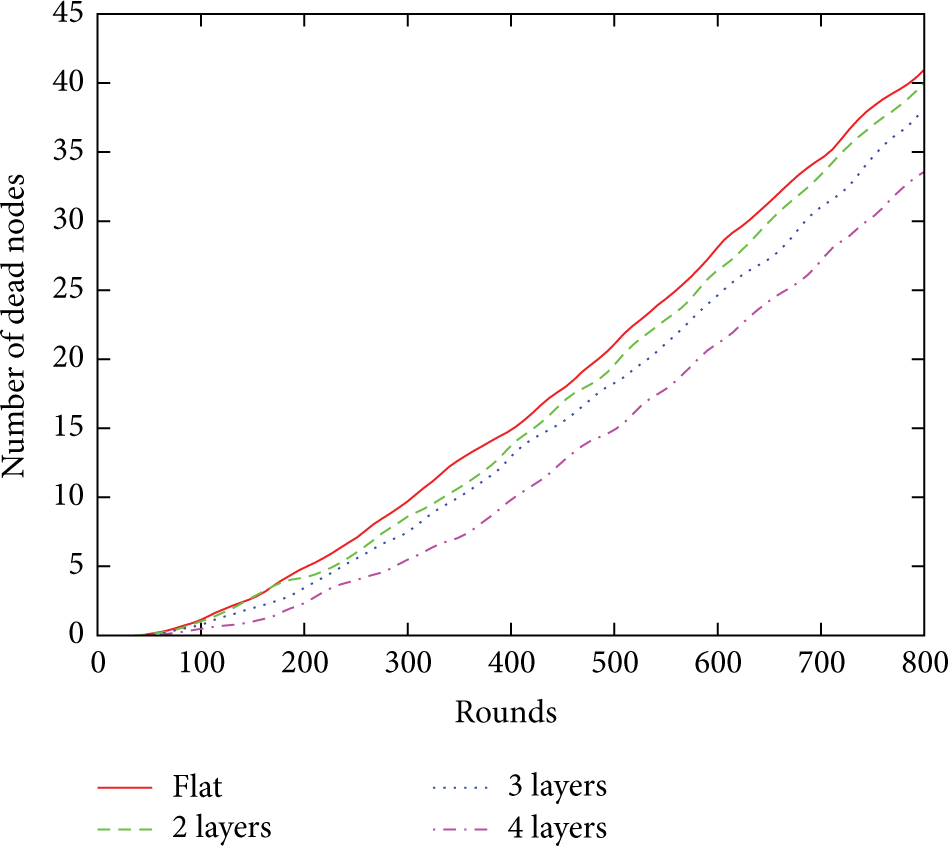
Change in the number of dead nodes without replacement.

Figure 6

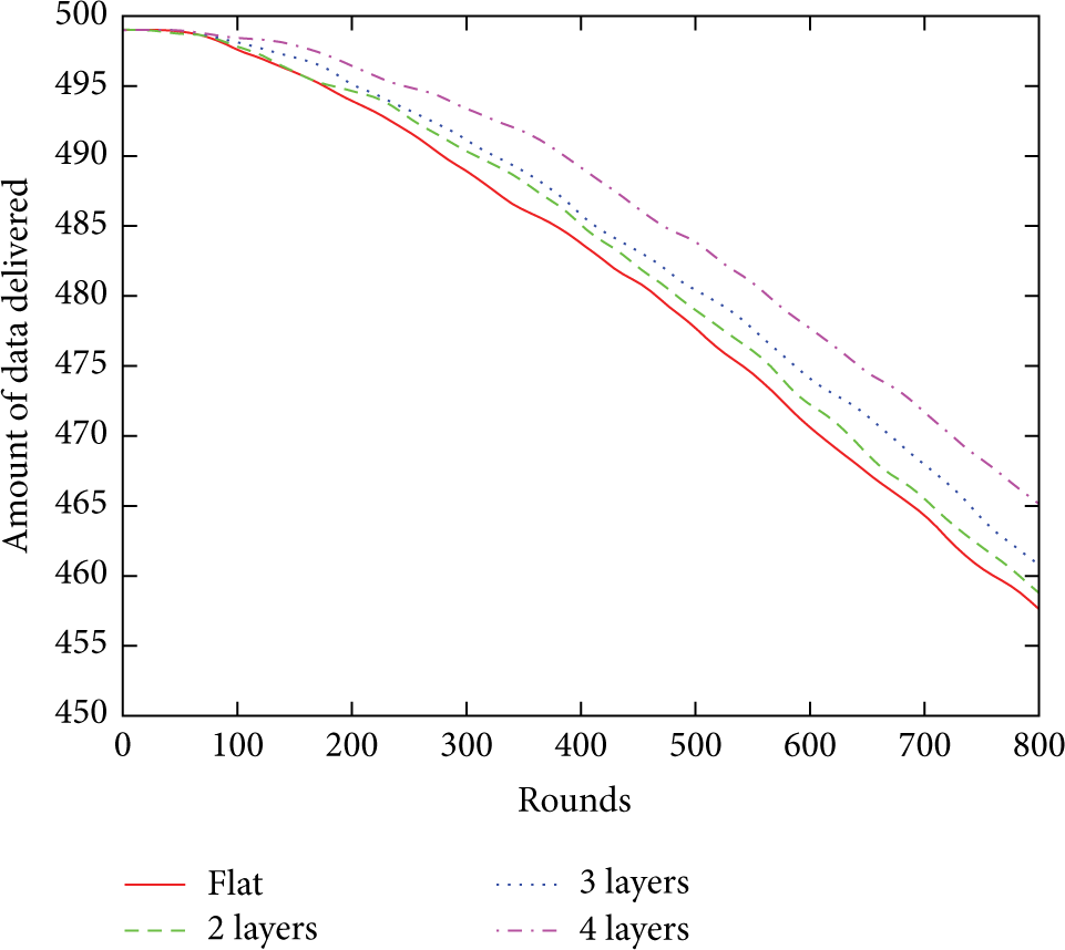
Change in the amount of data gathered at the sink node without replacement.

Figure 7 traces the number of defunct nodes over time in the network, in a scenario in which dead nodes are replaced with new nodes at every 200 rounds. This resulting sawtooth curve results in the pattern of Figure 5 as the network is refreshed by new nodes with fully changed batteries. Figures 8 and 9, respectively, show the number of dead nodes and the amount of data that arrived at the sink node, as the replacement period was varied from 100 to 300. The flat topology causes more nodes to die and data transmission is less effective than it is with the layered topology. The effectiveness of transmission declines as the redeployment period increases, as we would expect, because dead nodes are waiting longer for replacement.

Figure 7

Variation in the number of dead nodes with periodic replacement.

Figure 8

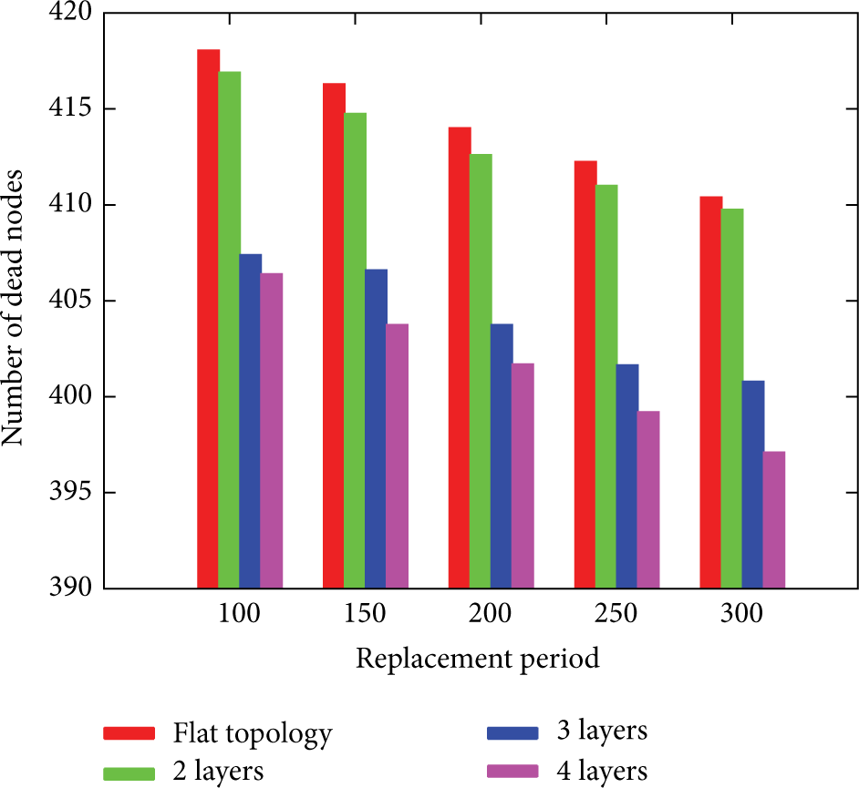
Variation in the number of dead nodes with the replacement period.

Figure 9

Variation in the amount of data arriving at the sink node with the replacement period.

Figures 10 and 11, respectively, show the number of dead nodes and the amount of data delivered to the sink. In this simulation, we assume that the network consists of only battery-powered nodes, and each node was a naive data aggregation scheme. Nodes aggregate the data received from the nodes in lower layers with their own data before sending it to their target node. The size of the resulting packet can be reduced omitting the headers of the packets received from lower-layer nodes; and the effectiveness of data aggregation is proportional to the size of a packet header. As shown in Figures 10 and 11, our scheme shown reduces the number of dead nodes by about 10% and delivers slightly more data than the flat topology.

Figure 10

Number of dead nodes with data aggregation.

Figure 11

Amount of data arriving at the sink node with the data aggregation.

In order to analyze the effectiveness of our scheme in networks with energy-harvesting nodes, we measured the number of dead nodes and the amount of transmitted data in a network consisting of 90% battery-powered nodes and 10% of energy-harvesting nodes. As shown in Figure 12, the number of dead nodes is reduced by about 10% by our scheme, which is very similar to the result for the network with only battery-powered nodes. Figure 13 shows that our scheme also delivers more data. However, it also shows that the effectiveness of transmission is sometimes reduced by the presence of energy-harvesting nodes. We suggest that this is because the energy-harvesting nodes are not replaced, even when they have little energy; instead, they wait for energy to arrive and charge their batteries. Meanwhile transmissions are failing. We also found that using energy-harvesting nodes as cluster nodes produces the least effective transmission of data. Again, we attribute this to the amount of energy acquired by these nodes, which is inadequate to transmit lots of data. This problem may be addressed by increasing the size of solar panels fitted to energy-harvesting nodes, or reducing the proportion of these nodes that are deployed.

Figure 12

Variation in the number of dead nodes as the proportion of energy-harvesting nodes is increased.

Figure 13

Variation in the amount of data arriving at the sink node as the proportion of energy-harvesting nodes is increased.

5. Future Work

The routing algorithm adopted in this paper causes a node to choose the route that reaches a higher-layer node with the minimum hop-count: only the length of routes is considered, not the residual energy in the nodes on those routes or their contribution to overall network connectivity. Therefore it does not explicitly contribute to the lifetime or connectivity of a network. We believe that it should be possible to design a routing scheme for layer-based topology control which makes a greater contribution to overall network efficiency.

The aggregation scheme reported in this paper is naive, in that it only aggregates data delivered from lower layers. More efficient data aggregation or fusion schemes have been described [27–30], and we intend to adopt one of them to reduce the volume of data to be transmitted and hence increase the lifetime of a WSN.

6. Conclusions

Since the nodes in a WSN are connected to the sink node by multihop routes, the demise of intermediate nodes reduces the amount of data that reaches the sink. A lot of work by many researches has been put into topology control techniques to address this problem.

In this paper we have proposed a layer-based topology control scheme for WSNs consisting of many nodes, some of which are battery-powered and some energy harvesting. These nodes are arranged in layers on the basis of their residual energy. The nodes in the higher layers aggregate data received from lower-layer nodes and send it to the sink node, together with data obtained from their own sensor. This preserves the connectivity of the WSN, because the expected lifetimes of nodes are balanced by moving them between layers.