Sage Journals: Discover world-class research

Abstract

The huge amounts of data generated by media sensors in health monitoring systems, by medical diagnosis that produce media (audio, video, image, and text) content, and from health service providers are too complex and voluminous to be processed and analyzed by traditional methods. Data mining approaches offer the methodology and technology to transform these heterogeneous data into meaningful information for decision making. This paper studies data mining applications in healthcare. Mainly, we study k-means clustering algorithms on large datasets and present an enhancement to k-means clustering, which requires k or a lesser number of passes to a dataset. The proposed algorithm, which we call G-means, utilizes a greedy approach to produce the preliminary centroids and then takes k or lesser passes over the dataset to adjust these center points. Our experimental results, which were used in an increasing manner on the same dataset, show that G-means outperforms k-means in terms of entropy and F-scores. The experiments also yield better results for G-means in terms of the coefficient of variance and the execution time.

1. Introduction

Nowadays, healthcare data are received from various healthcare service providers including sensory environment to provide better healthcare services. This data contains details about patients, medical tests, and treatment. The received data is very vast and complex; thus, it is difficult to quickly analyze the data in order to make important decision regarding patient health. Data mining technique is one of the important research areas in identifying meaningful information from huge datasets. In healthcare application, such as a heart monitoring system, it is an important method for efficiently detecting unknown and valuable information from huge heterogeneous health data. In a healthcare application, data mining techniques can be used to detect unknown diseases, causes of diseases, and identification of medical treatment methods. It also helps medical researchers in making efficient healthcare policies, constructing drug recommendation systems, and developing health profiles of individuals [1].

In order to analyze and extract meaningful information from this complex data a powerful computing tool is necessary. The outcome of data mining technologies is to provide benefits to a healthcare organization for grouping patients having similar type of diseases or health issues so that the organization can provide them with effective treatments. Various data mining techniques such as classification, clustering, and association are used by healthcare service providers for making a decision regarding patient health conditions.

Classification is one of the well-known and used techniques of data mining in healthcare data analysis. The data classification approach predicts the target class for each data point; for example, a patient can be classified as “high risk” or “low risk” depending on the basis of her/his disease pattern. There are different classification methods such as K-nearest neighbor (K-NN), decision tree, support vector machine (SVM), and ensemble approach that are used in classification techniques. Classification is mainly a supervised learning approach with the assumption of known class categories.

On the other hand, clustering is an unsupervised learning technique. Unlike classification, the clustering method has no predefined classes. In clustering, large datasets are partitioned into different small subgroups or clusters based on the similarity measure [2]. This approach is mainly used to find similarities between data points. Over the years various clustering techniques are developed and used. The main feature of clustering is that it needs less or no information for analyzing the data.

The k-means clustering algorithm is one of the widely used data clustering methods where the datasets having “n” data points are partitioned into “k” groups or clusters. The k-means grouping algorithm was initially proposed by MacQueen in 1967 [3] and later enhanced by Hartigan and Wong [4]. Bottou and Bengio [5] demonstrated the merging lands of the k-means calculations methods and algorithms methodologies. It has been indicated to be exceptionally handy for a corpus of commonsense provisions and widely used applications. The definitive k-means algorithm works with in-memory information, yet it could be effectively stretched out for out-of-memory occupant datasets.

The principal issue with k-means calculations is that it makes one probe over the whole dataset on each cycle, and it needs many such cycles before focalizing to a quality result. This makes it extremely costly to utilize, especially for substantially huge local disk datasets. Researchers have focused on lessening the amount of passes needed for k-means and, therefore, increase the performance of the algorithm. On the other hand, these methodologies just give surmised results, potentially with deterministic or probabilistic limits on the nature of the results. A key preference of k-means has been that it merges to a local minimum, which does not hold accurate for the estimated versions [2]. In this manner, an intriguing inquiry arises: can we have a methodology of calculation which obliges fewer passes on the whole dataset and can handle the same converging results as the fundamental k-means algorithm?

In this paper, we present one such algorithm, which we call G-means. G-means facilitates the calculation of the initial centroids using a greedy approach. The rest of the paper is organized as follows. Section 2 provides background on clustering algorithms. Section 3 presents related works. Section 4 offers our proposed approach. Section 5 discusses the experimental results, and Section 6 concludes the paper.

2. Background

k-means is one of the relaxed unsupervised erudition algorithms that illuminate the well-known clustering issue [3]. The methodology trails after a straightforward and simple approach to group a given information set through a certain number of groups (expect k groups) that have been established beforehand. The principle idea is to characterize k centroids, one for each group. These centroids have to be set in a guile manner resulting in a distinctive area of diverse effects. In this way, the better decision is to place them as far as possible from one another. The subsequent step is to take each point within a given information set and copartner it with the closest centroid until reaching a state where all the points have been associated with a group. Once the first stage is done and an unanticipated aggregating is carried out automatically, we need to reconfigure k new centroids as barycenters of each group due to the last step. After producing these k new centroids, another binding must be established between the same centroids set and the closest new centroid. A cycle will be produced. As an after effect of this cycle, we may recognize that the k centroids will change their regulated areas and at the end of the day centroids will not change their positions anymore [2, 6].

The objective function is shown below; and thus, the algorithm aims to reduce the squared error in this function:

\begin{matrix} J = \sum_{j = 1}^{k} \sum_{i = 1}^{n} {‖x_{i}^{(j)} - c_{j}‖}^{2} . \end{matrix}

(1)

The distance indicator of the n dataset points is

x_{i}^{(j)}

and their represented centroids

c_{j}

are

{‖x_{i}^{(j)} - c_{j}‖}^{2}

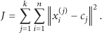
Methodically speaking, the k-means algorithm is composed of four steps and they are in the following order. (1)

Randomly place k elements in a space representing the items coordinates that are being clustered.

(2)

Allocate each item in the space to a group that is the most similar to it.

(3)

After the assignment of all the items in the space, recompute the k centroid elements and change their positions, respectively.

(4)

Repeat steps (2) and (3) until the centroids reach a position where they no longer change with respect to the distances between all the elements of their group.

Ultimately, the technique will dependably end; however, the k-means calculation does not usually find the most optimal design, or at least comparing it to the minimum global objective function that has been stated. The algorithm is delicate and fundamentally dependent on the beginning arbitrarily elected group centers. The algorithm should run at different times to decrease this impact though it will choose a different set of centroids each time, making it very hard to compare its initial indications [7]. Algorithm 1 depicts the k-means algorithm and its output.

Algorithm 1: The k-means algorithm and its output.

Algorithm: k-means. The k-means algorithm for partitioning, where each cluster's center is represented by the mean value of

the objects in the cluster.

Input:

k: the number of clusters,

D: a data set containing n objects.

Output:

A set of k clusters.

Method:

(1) randomly choose k objects from D as the initial cluster centers;

(2) repeat

(3) (re)assign each object to the cluster to which the object is the most similar, based on the mean value of the objects

in the cluster;

(4) update the cluster means, i.e., calculate the mean value of the objects for each clusters;

(5) until no change;

Figure 1 illustrates how the algorithm is run one step at a time. It demonstrates three groups in a space where k is equal to three, and they are distinguished according to the colors with their represented data elements (blue, brown, and green). For additional clarification they are isolated along three parts. Figure 1(a) is the initial centroids selection at random where k number of initial centroids have been depicted and accordingly coloring their entire group with the same color. The centroids are characterized by the plus sign.

Figure 1

(a) Initial centroids depiction. (b) Repositioning of centroids. (c) k-means converges.

In Figure 1(b) four iterations are concluded. The assignment of each element to its closest centroid is done by the distance calculation between the initial cluster centroids and every element in the space. The recalculation and deviation of the cluster centroids are computed at each iteration over this phase.

Figure 1(c) is where the algorithm converges, reaching a final position. This is reached when the algorithm compares the centroids from the last step to its current step and notices that there are no changes in the centroids; thus, the full clusters have been reached.

3. Related Works

Clustering is a fairly frequent but very important field of study, not only for computer scientists but also for statisticians and patterns recognition experts. There are vast researches on algorithms that have been developed or enhanced; we only focus on the works related to our topic of interest.

An intriguing discovery was achieved by Pelleg and Moore [8, 9] where they proposed a variant to k-means using a methodology called KD tree. This is formed using a regular tree algorithm, but it has a special data structure to store the distances between the nodes, which decrease each cycle of k-means significantly. However, it does not take into consideration the number hits made to the disk nor the number of reads to the database.

Bradley et al. [10] developed an algorithm based on k-means. It is a fairly scalable implementation of k-means, yet the downside is that it is sequential in nature. Hence, it takes as much data as possible and pushes it into principle memory. This can be a huge burden on very large datasets as the algorithm cannot fit everything into memory. Even though the authors proposed a fairly complex compression algorithm to take into account the big data problem, it has not worked in most of the experimental test cases. Results from this algorithm have shown to be slower than the original k-means but will solve deadlocks produced by the original k-means [11]. A simplification to the Bradley et al. algorithm was developed by Farnstrom et al. [12] to have more compression force and to lower the memory usage. Their idea is not to hold everything in the main memory but to have only one-dimensional array for the correlation coefficient. This can speed up processing, yet it will only produce the centroid points, not all the clusters.

The hierarchical clustering algorithm by Forman and Zhang [13] builds a tree-like structure by incrementing its indexes and rescans the data on every iteration. Through this, a BIRCH is created, with a data structure called Cluster Feature Tree. The advantage of this tree is that each node has a triple attribute associated with it: the node number, the weight summation, and the weight summation-squared. However, the solution provided by the algorithm is an approximate solution only. The downside is that the size of the tree can be hard to manage on a large scale since if it does not fit into memory, then BIRCH will become unusable.

Another heuristically defined algorithm is CURE [14]. It is called CURE because it is suggested to be a cure for clustering very large databases. It uses random sampling, and then it partitions the data into smaller groups. Afterwards, it commences the calculations for each smaller group and compares the groups together. Subsequently, it will merge each two groups that have a similarity function less than a certain threshold and will pick up the centroid of the new group by recalculating the mean for all the points, exactly as k-means does. The algorithm keeps on looping until it finds all the corresponding clusters that cannot be merged anymore. The results produced provide only an approximate answer.

Nittel et al. [15] also proposed a heuristic algorithm for out-of-core clustering. The authors' idea is to split the data into the maximum that the main memory can handle and try to scan the entire memory only once then run the k-means algorithm on the data chunks accordingly.

Samatova et al. [16] created a statistical approach to parallel clustering; the algorithm is backed up by a data structure based on dendrograms. As the authors try to merge from a local dendrogram to a global one using each iteration of the algorithm to collect data and based on a previously defined threshold, the algorithm will keep on iterating until the threshold is reached. The algorithm was experimented on large datasets and was not efficient because the structure of the dendrogram kept on growing and at a certain point in time went out of memory. The significance of their approach is using parallel clustering, which means that not only one dendrogram but also multiples were being produced at a single run; when a dendrogram reaches a certain threshold that has been previously defined, it will be merged with other ones until they construct final dendrograms each of which is considered a cluster, and the root of the tree-like structure is the centroid. A fairly similar approach was attempted by Parthasarathy and Ogihara [17], starting from the bottom up, yet dealing with distance metric formation by applying an association rule to the localized data. A high dimensional clustering with the help of distributed clustering combined the work of Kargupta et al. [18] and Januzaj et al. [19] yet the later one initiated the idea of converging from a local cluster into a global one, taking into consideration multiple clusters formation. These algorithms, however, do not end up producing an exact solution.

Fradkin and Madigan [20] developed a variation of k-means clustering to compress images which they called “divisive k-means.” Their approach requires very powerful machines to get accurate results.

In the advancement of clustering and computational power, there were many trials to parallelize k-means. Some of these works that relate to CLARANS [21] and BIRCH [13] deal with memory allocation and heuristics. Yet most of the clustering is done in one of two ways, either partitional or hierarchical. These approaches deal with all the data that needs to be clustered, yet some of the techniques filter the data before performing the actual clustering to minimize the size of the dataset first and then enhance the resulting clusters.

A recent framework proposed by [22] is to divide the clustering methodology into several stages. The work tailors streamed data. Their algorithm stores statistical information about the upstream data while another process sums up the collected information according to certain criteria characterized by the k constant number of clusters and the records per frame. It is a pyramid-like approach that keeps collecting the offline data and keeps a portrait of each cluster at a preference time frame. The experimental work conducted on a real database showed promising results in both efficiency and accuracy of the proposed solution.

Arthur and Vassilvitskii [23] propose a way of initializing k-means by choosing random starting centers with very specific probabilities. The authors select a point p as a center with probability proportional to p's contribution to the overall potential, leading to the algorithm k-means++. The authors provided preliminary experimental data showing that, in practice, k-means++ outperforms k-means in terms of both accuracy and speed.

Celebi et al. [24] investigate the initialization methods developed for the k-means algorithm. The authors demonstrate that the eight most popular initialization methods often perform poorly and that there are alternatives to these methods.

Himanshu and Srivastava [25] implemented a document clustering technique using singular vector decomposition to find out the number of clusters required (i.e., the value of k). The authors used the k-means algorithm to create clusters. These clusters are then refined by feature voting. This refinement phase enabled the algorithm to run more efficiently than the classic k-algorithm.

Polczynski and Polczynski [26] labelled common methods for classifying choropleth map features which typically form classes based on a single feature attribute. This methodology note reviews the use of the k-means clustering algorithm to perform feature classification using multiple feature attributes. The authors describe the k-means clustering algorithm and compare it to other common classification methods. The authors also provide two examples of choropleth maps prepared using k-means clustering.

4. The Proposed Approach

The essence behind our algorithm, G-means (with the G from the Greedy algorithm and the means from k-means since we use the same distance and similarity functions), is to facilitate the calculation of the initial centroids using a greedy approach; we believe that the k-means’ original algorithm needs improvement with the initial random selection of the centroids array. Hence, our initial step is to calculate all of the existing elements that have the highest degree in the space; from there we can have an initial configuration of what the clusters should look like. On the second run, we eliminate all the centroids that are in a single cluster and select k clusters with the highest results of the similarity function to be taken as the real cluster centroids. This being done, we iterate on the rest of the data elements to see if the centroids are going to change. This will be performed exactly like the original k-means with both the distance and similarity functions [27, 28].

The given input to the G-means algorithm is a graph G(V, E) and a constant k where V is the set of vertices (elements in the graph) and E is the set of edges (connections between the vertices), also noting that G is an undirected graph, which is the maximum number of clusters that should be generated [29]. The computational steps of G-means are as follows. (1)

The initial step is to pass through the entire dataset and identify the points with the highest degrees (i.e., the points that are the most close to the neighboring points). This constitutes the greedy part in the algorithm.

(2)

Compare these elements and consider how they are according to k number of clusters. Then, choose the k highest number of vertices.

(3)

Read through the entire database, without going over the elements of the centroid array, and check the similarity and distance functions from each centroid in the clusters to all its elements.

(4)

Each element that is read has either one of these options (with either the distance or similarity functions):

(a)

to be placed in the same cluster as the centroid array, thus dropping it, and the algorithm will never pick it up again;

(b)

to be kept for later lookup for a potential centroid (at a later run) since the distance function is indicating that it should be in another cluster;

(c)

to replace the current centroid and, thus, will win both the similarity and distance vector (since we are taking the highest degree element; this is a very rare case where both elements could be centroids, yet the k integer is smaller than the number of clusters).

(5)

The algorithm will keep on iterating and keep taking into account the (4(b)) part of the algorithm where these points could end up to be what is called “Boundary Points” of each k cluster.

(6)

If the run does not change anything in the centroids array, then we declare that it has successfully converged and display the centroids array.

(7)

To display each cluster, loop once through the centroids array and match the centroids color with the elements colors as to display the entire group.

4.1. Pseudocode

The pseudocode of the algorithm is shown in Pseudocode 1.

Pseudocode 1

Input: Graph $G (V, E)$ and constant k

Output: k cluster centers

Begin

CentriodsArray $[k] [$ Vertices]← NULL;

ColorArray[Vertices] ← NULL;

Read entire dataset;

Create the DegreeArray array;

Create a variable for number of runs called Runs;

For each k Do

GetMax(DegreeArray);

Add CentriodsArray $[k] [0]$ = Vertex;

Set the degree of the vertex to $- 1$ ;

Set the color array of the vertex to j;

Increment j and Runs;

Decrement k;

End

While Runs != k OR ColorArray has zeros Do

Read the entire dataset;

Identify the neighbors of the centroid elements;

Color them color the same as the centroid;

If neighbor is a centroid or an item is a centroid

Add CentriodsArray[Centroid $] [$ Vertex] = Vertex;

End

For each k Do

ResultsArray $[k]$ = CentroidArray $[k] [0]$ ;

End

Output ResultsArray;

End

4.2. An Example

In this section, we demonstrate how the proposed algorithm works through two examples. In both examples, we use the same number of elements, but the difference will be the k constant number of resulting clusters and the number of centroids. Figure 2(a) represents the initial state of the connected graph. Each rounded point represents an element in this space.

Figure 2

(a) Initial cluster space. (b) Initial centroids selection. (c) Centroids selections $K = 3$ . (d) The algorithm converges. (e) Centroid selection problem. (f) Correct centroids selection. (g) Algorithm converges.

In the second part, the algorithm picks up the total elements with highest degree regardless of k. Figure 2(b) illustrates these selections with the rounded red mark.

The algorithm will now compare the centroid selection with the constant k to give a precise number of elements in the centroids array. We consider two examples: the first when k would be equal to three and the next when k is equal to four.

Figure 2(c) denotes the centroids pickup when k is equal to three. The selection was made according to the distance function and the highest number of elements inside each group. The new centroids are the elements circled in purple.

For the purposes of this example, we assume that the centroids are not going to change, yet when the algorithm runs, it will color each of the elements to its corresponding centroid. Figure 2(d) depicts that the algorithm has successfully converged, resulting in three clusters and their centroids colored in black. Their unique shape defines each cluster.

The next example is constant $k = 4$ . We illustrate in this example how the distance and similarity functions come into the picture where they play a very important role in choosing the resulting centroids. The initial centroids selections are not going to change, yet the change is going to reside in the second step where the centroids are being compared to the constant k. Figure 2(e) shows that the algorithm faces a dilemma where the chances are the same for both of the points circled in red.

This is a common problem in all the greedy approaches where each element has the same number of connected nodes. But in this case, the similarity functions get in the way where both of the neighboring elements of point $(6,5)$ are centroids yet point $(5,4)$ has an element that is not a centroid. And if the first element is picked up, then the resulting cluster will be based on a single element; thus, the algorithm will pick up the second element and denotes it as a centroid in the centroids array. Figure 2(f) shows the correct selection of the centroids according to the similarity function rules.

Figure 2(g) depicts how the algorithm converges, and the successful four clusters with their centroids are colored in black. Their unique shape defines each cluster.

5. Experimental Results

We compare the k-means and G-means according to the entropy of the algorithm, in other words, the program-size complexity from the pseudocode and the actual Java code (or the complexity of the algorithm and program size). Another comparison is called the F-score or F-measure complexity for measuring the test results accuracy. We also compare the coefficient of variance and the execution time. And, finally, we will compare both algorithms’ complexities using the Big O notation even if the variation of the algorithms is small compared to running time [30]. All of the tests are done in an increasing matter; this is to see how both are reacting with the given datasets.

The dataset corresponded to a survey where respondents were solicited to record up to 14 from their unsurpassed most loved movies. The exploration group classified their judged class as “fit” and arranged movies referred to by respondents. The type, characteristics, plots, and topics convey socially imparted significances, and those criteria are a regular rearranging mechanism (or heuristic) on which gatherings of people base their preferences. The classifications used are based on Litman's framework [31]. This involved utilizing the grouping strategies connected by the neighborhood motion picture rental stores and portrayals furnished by later film guides.

The survey was presented to 600 applicants. Applicants were divided into 295 males and 305 females, with ages ranging between 13 and 65; their educational background ranges from students in high school to holders of Masters Degrees. Their racial/ethnic identity was also captured and they are as follows: Asians totaling 102, Whites totaling 220, Hispanics totaling 162, and African Americans totaling 82 and 6 people did not specify any group.

The Movies Genre classifications that were introduced are action, adventure, animation, biography, comedy, crime, documentary, drama, family, fantasy, history, horror, musical, mystery, romance, sci-fi, sport, thriller, war, and western.

The information examination is introduced in the following manners [32, 33]: (1)

with regard to all the referenced movies (in all the future references designated as All Cited Films), all the correspondents and movies were referred to by the demographic locations;

(2)

with regard to all the referenced top movies (will be referenced as Top 25), respondents rank movies in this record as far as their recurrence of reference; occasionally, due to ties, certain Top 25 records will hold more than 25 movies; to utilize one tied film and not an alternate would just be an alphabetic choice; this manner was chosen to sporadically run over the point of confinement of 25 for purposes of delegate exactness.

For all the correspondences taken by the 600 applicants, the number of citations is 1,703; if we included the reoccurrences of the same movie, the citation would increase to 6,102. This concluded that the average of correspondent is around 10.7, taking into consideration the contrast between the cited movies referred to by assembling each and every demographic class with the reference to movie genre, gender, or ethnicity.

The first test is the program complexity-size in relation to an increase in the dataset size; this is what is called the entropy [34]. This is done by taking both algorithms and testing them on each set of data and noting down the results accordingly.

Figure 3 shows that when we increase the dataset size, the entropy increases and the quality of the cluster decreases in k-means. G-means, on the other hand, provides a consistent increase in the complexity of the application, yet the cluster quality did not decrease; this is because of the greedy approach; to have the same results each time we run algorithm on the same set of data.

Figure 3

Complexity comparison.

The second part of our comparison is the binary classification that is known as the F-score or F-measure. The F-measure considers both the precision and the recall of the test to compute the score [7]. This test compares not only the results accuracy, but also the performance of both algorithms. In the context of clustering, the f-measurement or precision of the resulting clusters, also called positive predictive value, is when comparing the resulting clusters to the actual classification of the real-world example [35]. When we get the results of, say, the first cluster, we compare it to the real example results and get the F-measure.

In the movies dataset we compared the results from the surveys sent to real people and how manual classifications were conducted versus the results of the clusters from the G-means and k-means algorithms. This comparison showed that G-means gave good measures in comparison with k-means, taking into consideration the error percentage that might also be in the manual classification. For example, in the surveys, we obtained three clusters so k (number of resulting clusters) is 3. We begin by taking each cluster and comparing it to the resulting clusters. The first cluster has 23 elements and the algorithmic cluster has 25 elements; consequently, and depending on the precision of error, we have a rate 23/25 = 92%. As we did in the earlier test, we held multiple tests and chose the mean for each one increasing the dataset size gradually.

Figure 4 depicts the comparison line between the results of k-means and G-means; since we are measuring the F-score, we notice that the G-means measure is higher than k-means and much more stable.

Figure 4

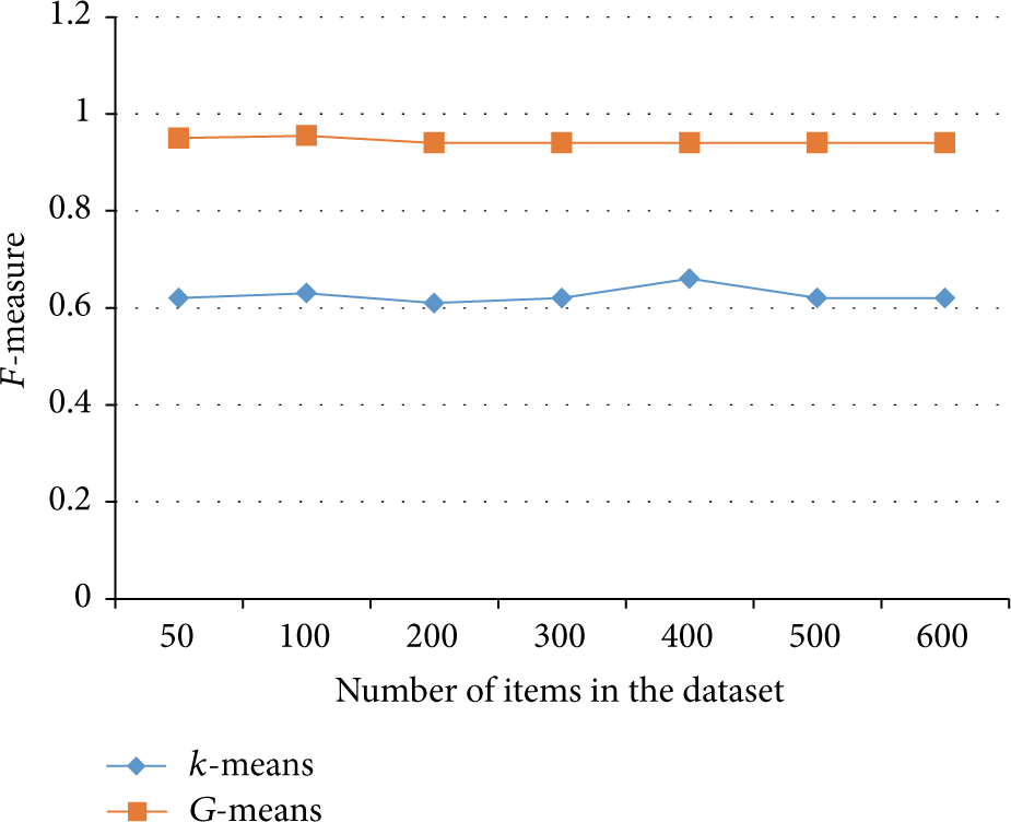
F-score of k-means and G-means.

We also compare the coefficient of variance; this is a very important measure statistically because it normalizes the whole algorithm (i.e., test the coefficient of variance without taking into consideration the complexity of the algorithm and the complexity of the datasets) [36]. The coefficient of variation is defined as the ratio of the standard deviation to the mean. It shows the extent of variability in relation to mean of the population.

Considering the same dataset and conducting simultaneous experimentation, we obtain the results depicted in Figure 5. The results show that whenever the datasets are large to reach (approximately from 5 or more k constant), then the variant for G-means drops drastically. This is because all of the factors in the algorithm have been rounded together to form this intriguing result.

Figure 5

Coefficient of variance of k-means and G-means.

Our next comparison deals with the execution time of each algorithm. The execution time is from the initial k constant determination until the algorithm converges, without taking into consideration any kernelization done before the start of the algorithm or any output design that should, for example, draw the clusters with their corresponding centroids. We differentiate the iteration by the number of elements inside each dataset as we increase the numbers gradually to see how the algorithms react to such cases.

The results, depicted in Figure 6, show that when we increase the dataset, the increase of the execution time for k-means is almost constant, yet the bulk running time of G-means becomes at the start much higher; as we increase the dataset, it is increasing at less time at each run. This is due to the fact that the G-means has a nearly constant time for initial centroid selection and cluster classification which at this stage takes a large amount of execution time. Also, the iterations that will follow the initial step are minimal; thus it is concluded that when the dataset number of items increases, G-means will start to converge faster than the regular k-means.

Figure 6

Running time of k-means and G-means.

The complexity of the G-means algorithm is represented as $O (n * k * i * d)$ where n is the number of elements, k is the number of clusters, i is the number of iterations, and d is the number of attributes. The notation can be simplified because k and d are constants and the number of iterations in a worst case scenario can be the same as the number of elements in the space. Thus, the formula can be reduced to a constant C multiplied by ( $n * n$ ). The final resulting function since the constant will be removed is $O (n^{2})$ . This is also the worst case of k-means; the only difference would be the constant that will be applied to it.

6. Conclusion

There are many research efforts devoted to clustering based on similarity matrices, yet there are no algorithms that use a greedy approach and get to the same or slightly different results as the k-means algorithm. In this paper, we presented a new technique that can cluster very large data whereby sometimes k-means could not, while minimizing the number of reads of the entire dataset. As for future work, we plan on forming a distributed version of the G-means algorithm, where data or even computational power could be spread over different remote machines. Another idea that we are currently contemplating is that most of the clustering algorithms deal with a constant k number of clusters, where in fact this hinders the basic idea of why we are doing the clustering. Consequently, we plan on directing our efforts towards handling a variable k instead of a constant one as this is very helpful in real-world examples where data is always changing and k cannot be fixed. We also plan to work on clustering algorithm kernelization; this means that both the algorithm and data taken should be preprocessed using specific rules so that they can enhance the performance and the results of the clustering algorithm.

Footnotes

Conflict of Interests

The authors declare that there is no conflict of interests regarding the publication of this paper.

Acknowledgment

This work was funded by the Lebanese American University, Beirut, Lebanon.

References

Koh

H. C.

Tan

Data mining applications in healthcare

Journal of Healthcare Information Management 2005 19 2 64 72

2-s2.0-19844377332

Kulis

Jordan

M. I.

Revisiting k-means: new algorithms via Bayesian nonparametrics

Proceedings of the 29th International Conference on Machine Learning (ICML '12)

July 2012

Edinburgh, UK

513 520

2-s2.0-84867132578

MacQueen

J. B.

Some methods for classification and analysis of multivariate observations

Proceedings of the 5th Berkeley Symposium on Mathematical Statistics and Probability

1967

University of California Press

281 297

Hartigan

J. A.

Wong

M. A.

Algorithm AS 136: a k-means clustering algorithm

Journal of the Royal Statistical Society, Series C 1979 28 1 100 108

Bottou

Bengio

Tesauro and

Touretzky

Convergence properties of the k-means algorithms

Advances in Neural Information Processing Systems 7 1995

New York, NY, USA

MIT Press

585 592

Jain

A. K.

Dubes

R. C.

Algorithms for Clustering Data 1988

Upper Saddle River, NJ, USA

Prentice Hall

Abrams

Hogg

Social Identity Theory: Constructive and Critical Advances 1990

Hemel Hemstead, UK

Harvester Wheatsheaf

Pelleg

Moore

X-means: extending k-means with efficient estimation of the number of clusters

Proceedings of the Seventeenth International Conference on Machine Learning

2000

Palo Alto, Calif, USA

Pelleg

Moore

Accelerating exact k-means algorithms with geometric reasoning

Proceedings of the 5th International Conference of Knowledge Discovery and Data Mining

August 1999

San Diego, Calif, USA

277 281

10.1145/312129.312248

10.

Bradley

P. S.

Fayyad

Reina

Scaling clustering algorithms to large databases

Proceedings of the 4th International Conference on Knowledge Discovery and Data Mining

1998

11.

Zhang

Ramakrishnan

Livny

BIRCH: An efficient data clustering method for very large databases

In Proceedings of the ACM SIGMOD International Conference on Management of Data 1996 25 2 103 114

2-s2.0-0030157145

12.

Farnstrom

Lewis

Elkan

Scalability for clustering algorithms revisited

ACM SIGKDD Explorations Newsletter 2000 2 1 51 57

10.1145/360402.360419

13.

Forman

Zhang

Distributed data clustering can be efficient and exact

ACM SIGKDD Explorations Newsletter 2000 2 2 34 38

10.1145/380995.381010

14.

Guha

Rastogi

Shim

Cure: an efficient clustering algorithm for large databases

Proceedings of the ACM SIGMOD International Conference on Management of Data (SIGMOD '98)

June 1998

Seattle, DC, USA

73 84

10.1145/276304.276312

15.

Nittel

Leung

K. T.

Braverman

Dayal

Ramamritham

Vijayaraman

T. M.

Scaling clustering algorithms for massive data sets using data stream

Proceedings of the 19th International Conference on Data Engineering

2003

Bangalore, India

IEEE Computer Society

16.

Samatova

N. F.

Ostrouchov

Geist

Melechko

A. V.

RACHET: an efficient cover-based merging of clustering hierarchies from distributed datasets

Distributed and Parallel Databases 2002 11 2 157 180

10.1023/a:1013988102576

2-s2.0-0036495698

17.

Parthasarathy

Ogihara

Clustering distributed homogeneous datasets

Principles of Data Mining and Knowledge Discovery 2000 1910

Berlin, Germany

Springer

566 574 Lecture Notes in Computer Science

10.1007/3-540-45372-5_67

18.

Kargupta

Huang

Sivakumar

Johnson

Distributed clustering using collective principal component analysis

Knowledge and Information Systems 2001 3 4 422 448

10.1007/pl00011677

19.

Januzaj

Kriegel

H. P.

Pfeifle

Scaling clustering algorithms for massive data sets using data stream

Proceedings of the Workshop on Clustering Large Datasets (ICDM '03)

2003

20.

Fradkin

Madigan

Experiments with random projections for machine learning

Proceedings of the 9th ACM SIGKDD International Conference on Knowledge Discovery and Data Mining

August 2003

517 522

10.1145/956750.956812

2-s2.0-63249106662

21.

Ioannidis

Poosala

Balancing histogram optimality and practicality for query result size estimation

Proceedings of the ACM SIGMOD International Conference on Management of Data (SIGMOD '95)

1995

233 244

22.

Aggawal

C. C.

Han

Wang

P. S.

A framework for clustering evolving data streams

Proceedings of the 29th International Conference on Very Large Data Bases (VLDB '03)

2003

Elsevier

23.

Arthur

Vassilvitskii

k-means++: the advantages of careful seeding

Proceedings of the ACM-SIAM Symposium on Discrete Algorithms

2007

1027 1035

MR2485254

24.

Celebi

M. E.

Kingravi

H. A.

Vela

P. A.

A comparative study of efficient initialization methods for the k-means clustering algorithm

Expert Systems with Applications 2013 40 1 200 210

10.1016/j.eswa.2012.07.021

2-s2.0-84866127615

25.

Himanshu

Srivastava

k-means based document clustering with automatic ‘k’ selection and cluster refinement

International Journal of Computer Science and Mobile Applications 2014 2 5 7 13

26.

Polczynski

Using the k-means clustering algorithm to classify features for choropleth maps

Cartographica 2014 49 1 69 75

27.

Berkhin

A Survey of Clustering Data Mining Techniques 2006

Sunnyvale, Calif, USA

Springer

28.

Silvia

Kelvin

T. L.

Braverman

Scaling clustering algorithms for massive data sets using data stream

Proceedings of the 20th International Conference on Data Engineering

April 2004

IEEE

10.1109/ICDE.2004.1320061

29.

Haraty

Mansour

Daou

Siau

Regression test selection for database applications

Advanced Topics in Database Research 2004 3

Hershey, Pa, USA

Idea Group Publishing

141 165

10.4018/978-1-59140-255-8.ch008

30.

Bradley

P. S.

Fayyad

Reina

Scaling clustering algorithms to large databases

Proceedings of the 4th International Conference on Knowledge Discovery and Data Mining

1998

31.

Litman

B. R.

Predicting success of theatrical movies: an empirical study

The Journal of Popular Culture 1983 16 4 159 175

10.1111/j.0022-3840.1983.1604_159.x

32.

Andrews

Film: the great divide; the sexes at the box office

New York Times 1993 2 15

33.

Austin

B. A.

Motivations for movie attendance

Communication Quarterly 1986 34 2 115 126

10.1080/01463378609369627

34.

Moore

A. W.

Efficient memory-based learning for robot control

University of Cambridge. Development Report website, 1991, http://www.cl.cam.ac.uk/techreports/UCAM-CL-TR-209.html

35.

Mansour

Haraty

R. A.

Daher

Houri

An auto-indexing method for Arabic text

Information Processing and Management 2008 44 4 1538 1545

10.1016/j.ipm.2007.12.007

2-s2.0-44449106061

36.

Dries

E. J.

Peterson

G. L.

Scaling ant colony optimization with hierarchical reinforcement learning partitioning

Proceedings of the 10th Annual Genetic and Evolutionary Computation Conference (GECCO '08)

July 2008

Atlanta, Ga, USA

BiblioBazaar

25 32

2-s2.0-57349179041

An Enhanced k -Means Clustering Algorithm for Pattern Discovery in Healthcare Data

Abstract

1. Introduction

2. Background

Algorithm 1: The k-means algorithm and its output.

3. Related Works

4. The Proposed Approach

4.1. Pseudocode

Pseudocode 1

4.2. An Example

5. Experimental Results

6. Conclusion

Footnotes

Conflict of Interests

Acknowledgment

References