Passive Diagnosis for WSNs Using Time Domain Features of Sensing Data

Abstract

Due to the dynamic network topology and limit of resources, fault diagnosis for wireless sensor networks is difficult. The existing diagnostic methods consume a lot of communication bandwidth and node resources, which lead to heavy burden of the resources limited network. This paper presents a passive diagnosis method used for fault detection and fault classification based on the time domain features of sensing data (TDSD). Firstly, the feature extraction and analysis of the sensing data are carried out using one-dimensional discrete Gabor transform, and then the data are diagnosed and classified with Self-Organizing Maps (SOM) neural network; finally the current network status and identifying the fault cause are determined. The results show that, comparing with other methods, this method has fewer burdens in network communication, better diagnostic accuracy rate and classification results, and so forth, and it has a high diagnostic accuracy especially for both node fault and network fault.

1. Introduction

Wireless sensor networks (WSNs) usually work in specific work environments. The sensor nodes are randomly deployed mostly in inaccessible environment. After deployment, node locations are so dispersed that it is too difficult to get close again. It is hard for the managers to detect or maintain each node. The large number of network nodes, the diverse types of sensors, the dynamic nature of the network topology, and the hierarchical deployment methods bring new challenges to the diagnosis for sensor networks. It is extremely important to diagnose the wireless sensor network timely and accurately. GreenOrbs [1, 2] is a large-scale WSNs system deployed in forest environments up to 330 sensor nodes. Nodes get sensing data at regular time. Once a node or network breaks down this will bring the system a huge impact, so it is necessary for GreenOrbs to diagnose fault.

There are many mature commercial diagnostic tools for troubleshooting enterprise networks, such as IBM's Tivoli [3], HP's Open-view [4], and Microsoft's Operations Manager [5]. These tools acquire large amounts of complex data by software agents, which is very effective for fault diagnosis of large-scale networks. But for resources and energy constrained wireless sensor networks, the calculation is too complex and has too large cost of energy to bear, and WSNs dynamic, self-organizing feature also limits the use of these tools. Active diagnostic process requires transferring large amounts of status information and specific control commands, such as network troubleshooting device sympathy [6] and diagnostic systems clairvoyant [7], focusing on detecting and tracking the software fault of sensor nodes, which tends to give the network the heavy burden. Passive diagnosis of sensor nodes meets the feature of limited resources and has little impact on the network's normal data collection, which is suitable for WSNs’ application requirements of low-power and efficiency. Articles [8–10] are introduced passive diagnostic methods in WSNs fault diagnosis. Liu et al. [8] proposed a probabilistic diagnosis (PAD) algorithm, using the network status parameter probabilistic model for WSNs diagnosis, but the method was complicated and inefficient diagnostic. Nie et al. [9] proposed a diagnosis based on sensing data (DSD) algorithm for fault diagnosis, but the algorithm did not consider the impact of the time domain. Miao et al. [10] proposed a line of lightweight fault diagnosis of Agnostic Diagnosis (AD) algorithms. Algorithm for static faults had good diagnostic results, but not for dynamic fault diagnosis.

To solve the above problem, in troubleshooting of a wireless sensor network, we further propose a TDSD algorithm, a passive diagnostic method which uses the domain feature of perception data to detect fault and classify the fault. Combining with the discrete Gabor transform and SOM neural network technology, this algorithm can effectively carry out fault detection and classification.

Our paper is divided into the following sections: Section 2 is to introduce the related work; Section 3 describes the TDSD algorithms framework; Section 4 is the experiment and analysis; Section 5 is the conclusion.

2. Related Work

2.1. Sensor Network Failure

The type of wireless sensor networks failure is usually divided into three categories: node failures, network failures, and software faults.

2.1.1. The Node Failure

Since large-scale wireless sensor network has a huge amount of nodes, deploying in harsh outdoor environments, the sensor nodes are easily damaged or destroyed. At the same time, due to the limited energy of nodes, the power failure occurs commonly; thus the failure rate is relatively high. The hardware problems of sensor nodes can also cause reading and other related troubles, so the node failure is subdivided into a node failure (caused by low voltage) and sensor fault.

2.1.2. The Network Failure

Network failure means that the network device or network service is not in a normal state. Generally network failures include network congestion, link failure, and loop. The network failures occur frequently in the region of the expression.

2.1.3. The Software Failure

The WSNs software failures typically include operating system crashes and other problems caused by the program bug. Once the software failure happened, this will bring great influence to the WSNs. In mature large-scale WSNs, the probability of occurrence software failure is relatively small.

2.2. Sensor Network Failure Diagnosis

About data collection and time domain feature, many people have made a lot of research. Article [11] proposed a novel packet delivery mechanism called Multipath and Multispeed Routing Protocol for probabilistic QoS guarantee in WSNs. It significantly improved the effective capacity of a sensor network in terms of number of flows that meet both reliability and timeliness requirements. Article [12] first proposed a multipath scheduling algorithm for the snapshot data collection in single-radio multichannel WSNs. This method significantly speeded up the data collection process. Article [13] studied the special issue of time synchronization in tiny sensor networking devices and proposed a Delay Measurement Time Synchronization (DMTS) technique applicable for both single hop and multihop WSNs. For a multihop WSN of n nodes, DMTS required N time message exchange in total in order to synchronize the whole network. It was a service available to TinyOS applications. Article [14] derived a general formula for the lifetime of wireless sensor networks which hold independently of the underlying network model including network architecture and protocol, data collection initiation, lifetime definition, channel fading characteristics, and energy consumption model. Based on this formula, they proposed a medium access control protocol that exploited both the channel state information and the residual energy information of individual sensors. Article [15] instead of using traditional spectral or wavelet techniques to extract a feature vector, representative of each vehicle, a time domain feature extraction method is adopted. These matrices could be used to train an Artificial Neural Network (ANN) to classify different types of vehicles.

Mahapatro and Khilar [16] integrated research efforts that had been produced in fault diagnosis specifically for wireless sensor networks. It had important reference value. The sensor network diagnosis usually sends diagnosis metrics which are from sensor nodes to the centralized sink periodically. Some existing approaches mainly rely on proactive approaches. For example, article [17] was a groundbreaking work in wireless sensor network diagnostics. They used tree-based heuristic reasoning to infer the cause of fault and diagnosed the state of nodes and links and other network members by optimizing the selection of the most effective real-time status information. But periodic sampling method used in the article will bring heavy network load. Article [18] proposed a WSNs dynamic model fault detection method based on Recurrent neural Network (RNN) for sensor node failure detection and classification, which had good efficiency of diagnosis contrasting with Kalman filtering. However, this method results in the diagnosis cannot achieve better accuracy.

Some other approaches used distributed diagnostic method; it reduced the transmission of information to the central node. Article [19] proposed a distributed online diagnostic method, using the remaining energy of the scanning sensor nodes to determine the working conditions of nodes and the network, reducing the data traffic and energy consumption. But the residual energy scan was only one kind of abstracted indication of sensor network state. Wang et al. [20] proposed a collaborative sensor fault detection (CSFD) algorithm to eliminate unreliable local decision-making in the implementation of distributed diagnostic fusion. The fusion rule predesigned established a probability of failure limit, assuming the local environment and the decision rules were the same. This method was too abstract and also not suitable for continuous large-scale WSNs diagnosis. Mahapatro and Khilar [21] proposed cluster-based distributed fault diagnosis (CDFD) algorithm. It considered the possibility of fault at different nodes of the network and the communication situations. Use sensor measurements spatial correlation, to get partial diagnostic view. But this algorithm may cause some fault-free node wrongly diagnosed as faulty.

The centralized diagnosis is relatively common fault diagnosis methods in WSNs. Ruiz et al. [22] proposed failure detection scheme using a management architecture for event-driven WSNs. Ramanathan et al. [6] used a tool for automatically diagnosing and aiding in the debugging of sensor network systems. The centralized diagnosis method is simple and convenient, but in large-scale WSNs it is difficult to apply.

The passive diagnosis method is suitable for large-scale WSNs application requirements of low-power and efficiency. The articles [8–10] focused on using passive diagnosis algorithm to diagnose the WSNs fault, from the different perspectives to research. All of the data from the GreenOrbs [8] used the network status parameter, [9] used the sensing data, and [10] used the system metrics, such as radio-on time, number of packets transmitted.

2.3. Gabor Transform

In 1946, D. Gabor [23, 24] proposed an approach which simultaneously uses time and frequency to represent a function of time Gabor Transform. It inherits the signal spectrum properties of the Fourier Transform while overcoming defect of Fourier Transform that it can only reflect the overall feature of the signal but cannot reflect the local feature of the signal. Gabor transform is widely used in feature extraction for signals. It simultaneously reflects the features of signals in time domain and frequency domain [25, 26]. Gabor transform can be described with the following formula:

$$\begin{array}{cc}& G_f={{\displaystyle \int }}_{-\infty }^{+\infty }f\left(t\right)g(t-\tau )e^{-iwt}dt,\end{array}$$

(1)

where $f(t)$ is the original function of the signal. The window function $g(t)$ is a smooth function. It constantly equals to 0 when it is in the outside of finite interval (i.e., having a function of compact support) or it quickly approaches zero. As Fourier Transform, $G_f(\omega ,\tau )$ , the Gabor transform of $f\left(t\right)$ also has inversion formula, the product theorem, and Parseval equation. The following equation is the inversion formula for Gabor transform:

$$\begin{array}{cc}& f\left(t\right)=\frac{\mathrm{1}}{\mathrm{2}\pi }{{\displaystyle \int }}_{-\infty }^{+\infty }{e}^{i\omega t}d\omega {{\displaystyle \int }}_{-\infty }^{+\infty }g\left(t-\tau \right)G_f\left(\omega ,\tau \right)d\tau .\end{array}$$

(2)

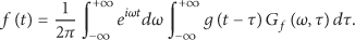
According to the definition of Gabor Transform, $G_f(\omega ,\tau )$ reflects the spectral feature of signal $f\left(t\right)$ in the vicinity of   $t=\tau$ . According to (2), $G_f(\omega ,\tau )$ does contain all the information of   $f\left(t\right)$ . In addition, the window position of Gabor transform with moves τ represents the local feature of the signal at different times.

2.4. SOM Neural Network

The Self-Organizing Maps (SOM) [27] neural network uses unsupervised learning method. According to its unique mesh structure and learning rules, by the repeated study of the input pattern, mode feature which is contained in each mode is captured. The classification results are expressed in the competition level after self-organizing. Thus, SOM is widely used in fault detection and classification [28, 29].

The maximum output neurons depend on the input $u^i={\sum }_{j=\mathrm{1}}^N{w}_{ij}{x}_j$ , that is the inner product of the input vector $X=(x_{\mathrm{1}},x_{\mathrm{2}},\dots ,x_N{)}^T$ and the weight vector $W={(w_{i\mathrm{1}},w_{i\mathrm{2}},\dots ,w_{iN})}^T$ ,   $i=1,2,\dots ,M$ . The inner product vector is equivalent to the input vector and the weight vector of the minimum Euclidean distance when the input and output vector are normalized vectors. Euclidean distance $d_j$ , that is, the Euclidean distance between the input sample and the output of each neuron j,

$$\begin{array}{cc}& d_j=‖X-W_j‖=\sqrt{{\displaystyle \sum }_{i=\mathrm{1}}^N{\left[x_i\left(t\right)-w_{ij}\left(t\right)\right]}^{\mathrm{2}}},\end{array}$$

(3)

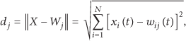
obtained a minimum distance of neurons and gave a neighborhood around $S_k(t)$ . According to (4) to amend the right value of the output neurons and the adjacent neuron

$$\begin{array}{cc}& w_{ij}\left(t+\mathrm{1}\right)=w_{ij}+\eta \left(t\right)\left[x_i\left(t\right)-w_{ij}\left(t\right)\right].\end{array}$$

(4)

3. TDSD Algorithms Framework

3.1. Preexperimental Results

In the fault diagnosis of wireless sensors, for a random node N, if there returns no data packet, the fault can be determined as communication equipment failure. If the data packet is returned, and the perception data is normal, then the node is working properly. As shown in Figure 1, the voltage value range of the selected data is about 2.8 V; the temperature and humidity change with time regularly. At about 13 o'clock the temperature reached a maximum value, while the humidity reached a minimum value.

Figure 1

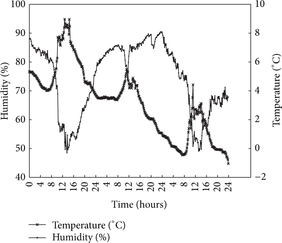
Variation of temperature and humidity in consecutive 3 days when the node is normal.

Voltage is an important influencing parameter in fault diagnosis for wireless sensor network. If the node voltage is abnormal, it will lead to the missing of data or data anomalies. A four-voltage division model (FLED) [9] is adopted to preliminary judge whether the voltage of a node is normal. As shown in Figure 2(a), in the case of low-power consumption, although there is fault in temperature data, it can still show its variation law currently. In Figure 2(b), when the voltage is ultralow, temperature fluctuations are abnormal, and there is no law to follow. When the battery runs out of energy, there is no data. When network congestion occurs, it will cause a large amount of node data anomalies. Data received at this time do not reflect any valid information of monitoring area, and there is great impact on the network. Figure 3 is the process that the temperature humidity and voltage of several nodes change from normal to abnormal and then return to normal during January 9 to 14 (we took the absolute values of data). In Figure 3, the black lines are normal except the concussion fault. During January 9 the data has severe concussion. The data transmission is abnormal. It stacked together; thus there is no rule to follow; this means there is a network failure. We can see the green line and yellow line, according to Figure 2, that is node failure (voltage fault) at this time, only collecting few data, the WSNs would be recovered well, and we must renew the battery supply. The blue lines in the upper part of the axis mean there is sensor fault (also because of the low voltage fault). When the network is normal, the data changes in a similar trend. That is because data from those nodes which are deployed in the same area has certain relevance, and there is no big difference in data.

Figure 2

The changes in temperature when the voltage is abnormal.

Figure 3

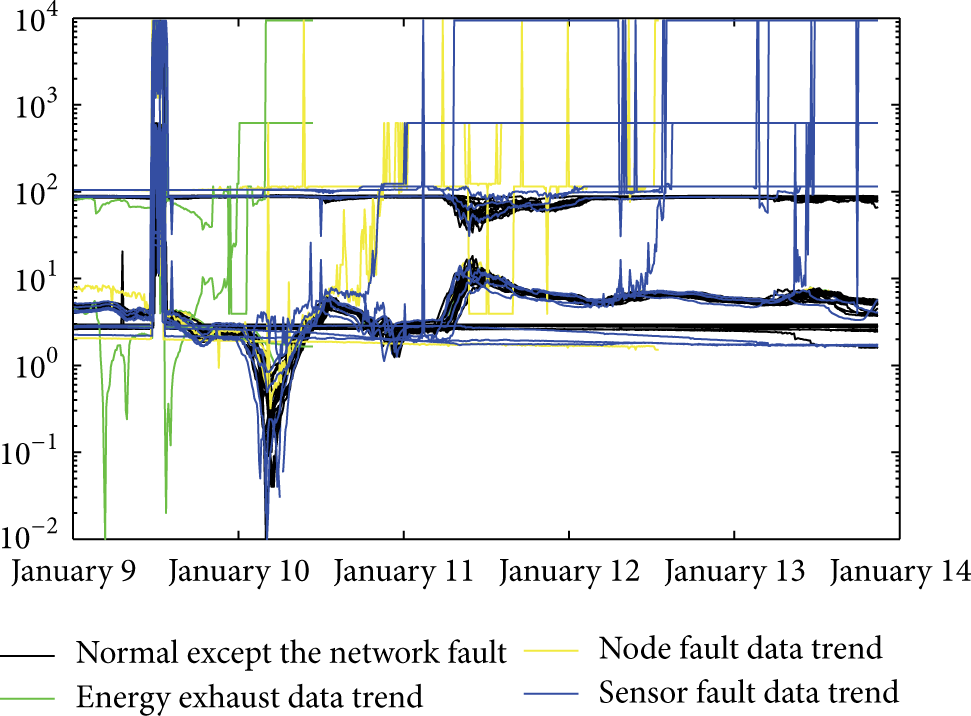
Node's time domain feature.

3.2. Algorithm Model

The existing studies show that improving the performance of fault diagnosis will increase the dimension of features space for the performance. However, in practice, the large number of extracted features does not mean a better diagnostic performance. In our experiments, the collected sensor data is discrete in both time and space.

• (1)

There are n sensor nodes, $n_1,n_2,\dots$ ; we define the set of the time sequence data flow X as follows:

$$\begin{array}{cc}& X=\left\{x_1,x_2,\dots ,x_n\right\}.\end{array}$$

(5)

 

$x_i$ represents the time sequence.

(2)

As adoption manual observation method to get the original fault data series fault of failure knowledge library $y(x)$ , it mainly includes H, T, and V parameters, representing the temperature and humidity and voltage.

(3)

Setting a threshold when detecting fault obtained a set of features of the signal $K(x)$ .

(4)

We define System $S=(A,K,g)$ ; among this, $A=C\cup D$ is the property set (C represents the set of characteristics of sensing data, D represents the set of failure types), K denotes the set of fault samples, and g is the result of clustering.

3.3. TDSD Algorithm

This paper presents a fault detection method based on features of perception data. The faults were detected and classified mainly through temperature, humidity, and other sensory data combined with the voltage data.

We combined the feature extraction and analysis of the sensing data with the one-dimensional discrete Gabor transform algorithm with SOM neural network, based on a series of rules failure knowledge library, monitoring the network performance, and finally the current network status and the fault cause are determined. In the algorithm framework as shown in Figure 4, the diagnostic process was in sink node, avoiding frequent reports of diagnostic parameters to reduce the network traffic load. At the same time this method reduces the dimensionality of data, avoiding the burden of diagnosis process caused by the variety of data, and improves the efficiency of diagnosis.

Figure 4

The architecture of TDSD model.

Before training the SOM neural network, the original fault data sequence $y(x)$ will do Gabor transform to obtain $G(x)$ . Second, the $G(x)$ was normalized to give $K(x)$ , then gave SOM neural network weights coefficient $W_{ij}$ any random value in the interval. After fault features vectors were sent into the neural network, we will find the best matching unit C for each input neuron between $K(x)$ and $W_{ij}$ . Then do the weight training according to (4). Repeat this process until all of the sample learning are completed. The algorithm is described as Algorithm 1.

Algorithm 1: Training.

   Input: $$y(x)=\{f_{\mathit{1}},f_{\mathit{2}},\dots ,f_j\}$$ ; % Training fault features samples

   Output: $$D=\{d\mathit{1},d\mathit{2},d\mathit{3},d\mathit{4}\}$$ ;

   % $$d\mathit{1}$$ : Node failure; $$d\mathit{2}$$ : Work well; $$d\mathit{3}$$ : Network failure; $$d\mathit{4}$$ : Sensor failure.

( $$\mathit{1}$$ ) $$y(x{)}_{\text{Gabor\_transform}}=G(x)$$ ;

   % Gabor transform for the training data

( $$\mathit{2}$$ ) $$G(x{)}_{\text{normalization}}=K(x)$$ ; % Normalization process

( $$\mathit{3}$$ ) Net = {SOM(T, H, V, M (m, m),  $$W_{ij},C)\}$$ ;

   % Establishment of SOM neural network: T, H, V denote the temperature and humidity and voltage

   conversion data; M is the number of neurons; $$W(ij)\in (\mathrm{0,1})$$ is net weight vectors; C is the best match unit;

( $$\mathit{4}$$ ) for trainparam.epochs $$i=$$ 100 : 100 : 500

   % Training Network steps

( $$\mathit{5}$$ )    $$yy$$ = sim(net, $$K(x))$$ ;

( $$\mathit{6}$$ )    $$\text{cluster\hspace{0.17em}1}(\mathit{1,2},\dots ,t)\in \text{class\hspace{0.17em}1}$$

      % Neurons clustering results

( $$\mathit{7}$$ ) end

( $$\mathit{8}$$ ) return   $$D=\{d\mathit{1},d\mathit{2},d\mathit{3},d\mathit{4}\}$$

After training the SOM neural network, all of the fault features vectors $K(x)$ information is memorized in the weight vector W, that the relationship between fault symptoms and fault data is implicit in the weight vector. We marked the maximum output neurons, winning neuron, depending on the location of the winning neuron distributions to determine the type of fault.

In this paper, the situation that no data is returned is classified into two cases:

• (1)

node never returns data, this can be judged as the communication link failure;

(2)

if there is historical data but no current data, it can be judged that the node has run out of energy.

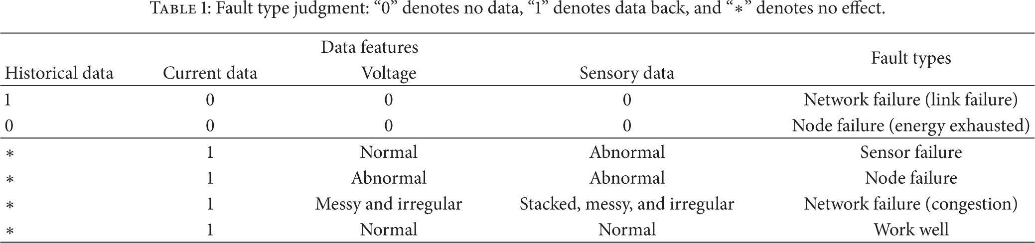
When there returns the experimental data, the failure can be divided into three types: the network failure, the node failure, and the sensor failure. The fault type judgment is shown in Table 1. The detailed algorithm is described as Algorithm 2; we assumed that the data can be transmitted back.

Table 1

Fault type judgment: “0” denotes no data, “1” denotes data back, and “∗” denotes no effect.

Data features				Fault types
Historical data	Current data	Voltage	Sensory data
1	0	0	0	Network failure (link failure)
0	0	0	0	Node failure (energy exhausted)
*	1	Normal	Abnormal	Sensor failure
*	1	Abnormal	Abnormal	Node failure
*	1	Messy and irregular	Stacked, messy, and irregular	Network failure (congestion)
*	1	Normal	Normal	Work well

Algorithm 2: Diagnosis.

   Input: $$Z(x)=\{x_{\mathit{1}},x_{\mathit{2}},\dots ,x_t\}$$ ; % Data to be detected

   Output: Fault diagnosis and classification results

   //Test data using Gabor transformation processing, normalization and then input to the SOM

( $$\mathit{1}$$ ) $$Z(x{)}_{\text{Gabor\_transform}}=G_z(x)$$ ;

   % Gabor transform for the data to be detected

( $$\mathit{2}$$ ) $$G_z(x{)}_{\text{normalization}}=K_z(x)$$ ;

   % Enter into the SOM neural network

( $$\mathit{3}$$ ) for  $$zz$$ = sim(net, $$K_z(x)$$ );

( $$\mathit{4}$$ )   $$\text{cluster}\hspace{0.17em}\text{2}(\mathit{1,2},\dots ,t)\in \text{class}\hspace{0.17em}\text{2}$$ ,

( $$\mathit{5}$$ ) end

   // Comparison of clustering results class 1 and class 2, fault type of data obtained and the results are classified

( $$\mathit{6}$$ ) match(class 1, class 2)

( $$\mathit{7}$$ ) if   $$\text{cluster\hspace{0.17em}2}\in (\text{class}\hspace{0.17em}\text{1}\cap \text{class}\hspace{0.17em}\text{2})$$

( $$\mathit{8}$$ )   if data is zero

( $$\mathit{9}$$ )    return  $$d\mathit{4}$$

( $$\mathit{10}$$ ) else

( $$\mathit{11}$$ ) if data is not zero

( $$\mathit{12}$$ )  if the readings are all irregular

( $$\mathit{13}$$ )    return  $$d\mathit{3}$$

( $$\mathit{14}$$ )  end

( $$\mathit{15}$$ )  else

( $$\mathit{16}$$ )  if voltage is abnormal

( $$\mathit{17}$$ )    return  $$d\mathit{1}$$

( $$\mathit{18}$$ )  end

( $$\mathit{19}$$ )  else

( $$\mathit{20}$$ )  if voltage is normal, readings is abnormal

( $$\mathit{21}$$ )    return  $$d\mathit{4}$$

( $$\mathit{22}$$ )  end

( $$\mathit{23}$$ )  else

( $$\mathit{24}$$ )    return  $$d\mathit{2}$$

( $$\mathit{25}$$ )  end

( $$\mathit{26}$$ )  end

( $$\mathit{27}$$ ) end

( $$\mathit{28}$$ ) if  $$\text{cluster2}\notin (\text{class}\hspace{0.17em}\text{1}\cap \text{class}\hspace{0.17em}\text{2})$$

( $$\mathit{29}$$ )  return  p  %p is the all clustering not belong

( $$\mathit{30}$$ ) End

4. The Experiment and Analysis

The experimental data derives from large-scale WSNs system, GreenOrbs. The data is collected once every 10 minutes by a sensor node and centralized to sink nodes by the WSNs.

4.1. Train

In the experimental stages of training, firstly, the failure data features of WSNs are transformed from the training data set by the meaning of Gabor. Then, the SOM neural network is used to train the normalized data to be clustered. After the training, the neural network clusters the data into several categories, which are on behalf of the different fault types. In the process of training, the number of clustering results by neural network is more than expected fault classification because the same type of fault data in WSNs has large differences. We divide the more than anticipated clustered outcomes in the process of the diagnosis so that the result of diagnosis can be showed obviously.

In our test, considering the efficiency and effect, we define the training steps for 500. At the same time, the effect of the size of neurons and training sample on the result is taken into account.

4.1.1. The Data of Training

We choose 400 fault samples as the data set of training, which contains all of faults we have found. In the fault samples, each type of fault data is distributed equally. Fault data is obtained by the method of artificial observation. Figure 5 lists the various fault corresponding color diagrams of some typical faults. In the drawing, the ordinate of each of the three lines indicates the temperature, the humidity, and the voltage of one node. The horizontal axis represents the node of temperature, humidity, and voltage, which change over the time. (a), (b), and (c), respectively, indicate the diagram of sensor fault, network fault, and node fault. We can see these data show a different disorder. However in (d), the normal data change smoothly and are sequential in the figure, and the gap of data in different nodes is also very weak at the same time.

Figure 5

The data of training clustering color map.

4.1.2. The Effect of the Neuron Size

During the SOM neural network training, the size of neurons has a great impact on the accuracy of fault diagnosis. In fault data samples, the number of each type fault is uniform distribution. In the experiment the faults can be divided into four kinds. When neurons selected for training fault are four, the fault samples cannot be well clustered. The error has great impact on results; thus the diagnosis is ineffective. That is because the fault samples differ greatly from each other; the impacts between the data cannot be well eliminated even if the samples were normalized. Therefore, only an increase in the number of neurons can improve the accuracy of clustering. But when the number of neurons is excessive, the types of fault increase. That will lead to an increase in training time. It is a waste of resource and has a low efficiency. Figure 6 shows the training polymerization accuracy under different neurons. The sizes of neurons are $3\mathrm{\ast }3$ , $5\mathrm{\ast }5$ , $6\mathrm{\ast }6$ , $8\mathrm{\ast }8$ , $10\mathrm{\ast }10$ , and $12\mathrm{\ast }12$ . In $10\mathrm{\ast }10$ neurons, the clustering effect has been very good, and then increasing the number of neurons has little effect on the diagnostic results. The training time gradually increases with the number of neurons. Therefore, after comprehensive consideration, under the condition that there are no special markers, this paper selects $10\mathrm{\ast }10$ neurons.

Figure 6

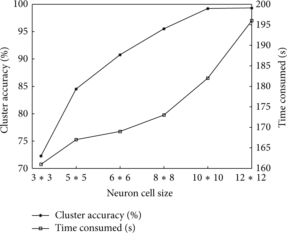
Effect of neuron cell size.

4.1.3. Impact of Fault Sample Size

During training, the size of the fault samples also has some impact on the diagnosis. In training, to detect an approach is effective or not, the aging problem must be taken into account. The sample sizes from 100, 200, 400, and 600 to 800 are selected for training cluster. With the increase of the sample size, the amount of time training has also increased, as shown in Figure 7. The results of this experiment have been repeatedly tested, which show that when the samples are 400, the basic known types of fault have been included and the diagnostic results for the different network size perform well. Of course, over time, the range of the data perceived by sample is large; then we have to update the knowledge base of fault sample. Without special markers, the size of fault sample is 400 in this paper.

Figure 7

Effect of fault samples size.

4.2. Diagnosis

The inputted sample data was diagnosed according to the fault knowledge base; the abnormal data can be detected and classified. There are two main indicators to weigh the merits of the algorithm: (1) fault detection rate and (2) fault false alarm rate. Fault detection rate is the percentage between the fault number detected by diagnostic algorithms and the total number of fault. Fault false alarm rate is the percentage to test the accuracy of the algorithm; we use the real data collected from the GreenOrbs system diagnostics and then detect the diagnostic algorithm with simulated data.

4.2.1. Diagnostic Results of Real Data

We selected the temperature and humidity sensing data as well as voltage characteristics of nodes for training, all of the data are from the GreenOrbs. Real data from different time periods during January 2012 was adopted as the diagnostic data; Table 2 shows the source of real data.

Table 2

The source of real data.

ID	Data Sources
R1	Data from 30 nodes during Jan. 7 to Jan. 8
R2	Data from 30 nodes during Jan. 13 to Jan. 14
R3	Data from 30 nodes during Jan. 15 to Jan.16
R4	Data from 30 nodes during Jan. 17 to Jan. 18

We classified the data according to the results of previous training. Figure 8 shows the classification results of the diagnosed data; the normal data is removed in this figure. The large differences in fault data triggered lots of neurons and thus led to a variety of classifications. Neurons which are triggered by most data are concentrated, and some are scattered. There is no effect on the diagnostic results. Meanwhile, we found that some data trigger no neuron. That is to say, they cannot be correctly classified, and these data are also figured out. In the real data of the diagnostic process, all types of faults generally do not appear at the same time.

Figure 8

Diagnostic results on real data classification.

4.2.2. Diagnostic Results of Simulated Data

We chose continuous stable operation nodes data to simulate the diagnosis. Fault data is obtained by the method of artificial observation; this includes all the known fault types corresponding to the fault data. In the experiment, to test the diagnostic performance of the algorithm, the minimum size of the selected network has 60 nodes and 10% of failure data is randomly implanted. The size of the network is 80, 100, 120, 140, and 160 nodes, respectively; each fault type is implanted equally to monitor the diagnosis performance under different network size.

Diagnostic results show that, with the increase in network size, the fault detection rate has not decreased, and the diagnosis effect is very good. When the network has 160 nodes, there is still high accuracy rate which is about 97.43%, which means a good diagnostic effect. This is because we have used multiple features for diagnosis. There is no need to set the threshold; we can get better effect according to the linkages between various parameters. Figures 9 and 10 have shown the fault detection rate and fault false alarm rate under different network size.

Figure 9

Fault detection rate.

Figure 10

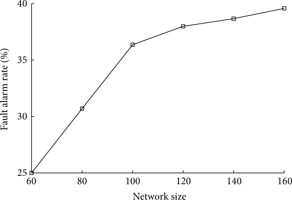
Fault false alarm rate.

The above results have shown that, with the increase in the number of network nodes and the fault samples, there is certain impact on the diagnostic performance of the algorithm, diagnosis effect when the network size increases, but the effect is little. As can be seen in Figure 10, with increase of network size, the fault detection rate gradually decreased, while false alarm rate gradually increased.

4.3. Diagnostic Results and Discussion

In previous GreenOrbs research work, PAD algorithm uses packet marking list to effectively build and dynamically maintain the reasoning model. Based on a large number of perception data, the DSD algorithm determines the type of fault through establishing a network failure knowledge base. Compared with the DSD method and Belief Networks (BN) inference models, Figures 11 and 12 are the comparison of fault detection rate and fault false alarm rate, respectively.

Figure 11

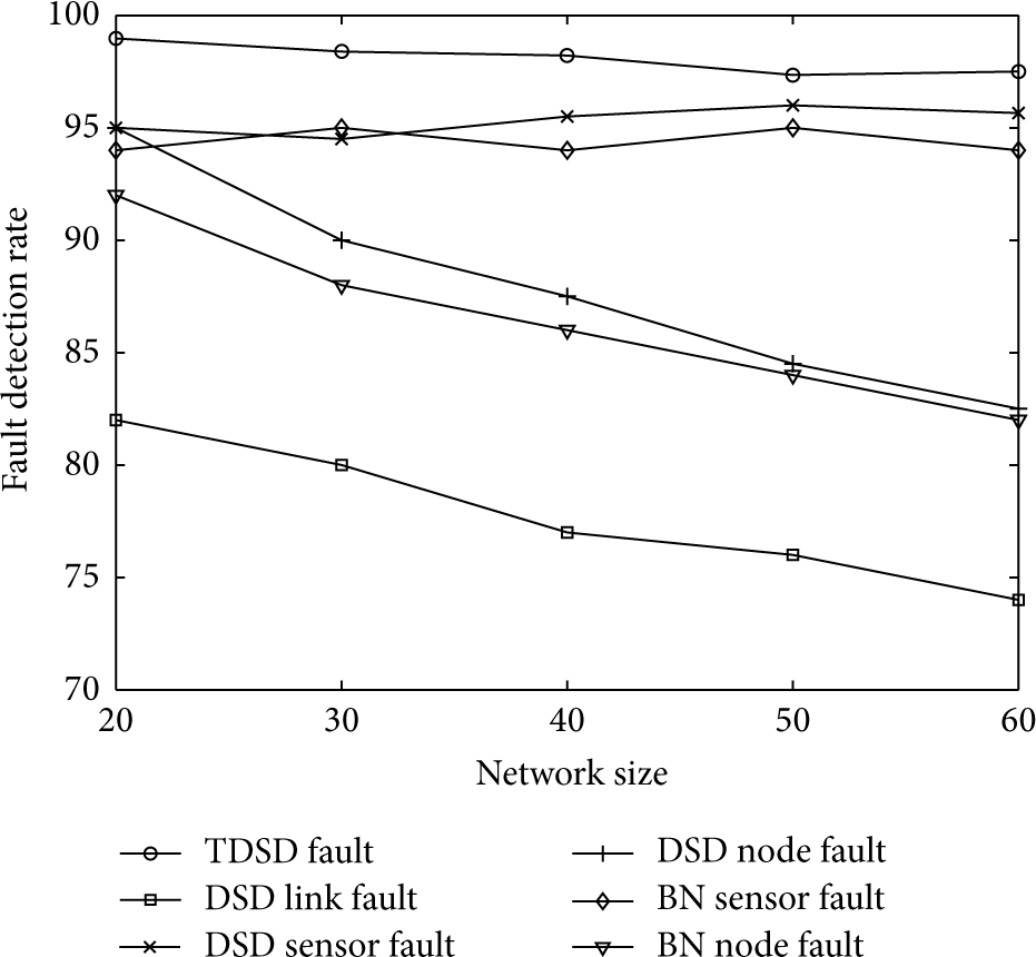
Fault detection rate.

Figure 12

Fault false alarm rate.

As can be seen from the graph, DSD algorithm and BN algorithm have the best results in fault detection for sensors; the detection rate is about 95%. Its false alarm rate decreases when the network size increases and it finally stabilizes around 35%. The fault detection rate for link failure and node failure is slightly lower. With the increase of network size, it ultimately stabilized around 75% and 82.5%; BN algorithm is only 20% false alarm rate for node failure. Algorithm in this paper is designed for the whole network. There are good diagnostic effects for those three kinds of fault types, so we will not discuss them separately. Our algorithm has better detection rates in large-scale WSNs diagnosis. Its detection rate is more than 97%. The false alarm rate is less than 40% when the network nodes reached 160.

5. Conclusion

Through the analysis of the data that GreenOrbs system collected within three months, diagnostic classification of the reasons for WSN fault was completed using the temporal feature of the perceptual data extracted by Gabor transform and fault knowledge established by SOM neural network to draw the network running. In this study, a better result of the overall diagnosis, as a large-scale network, was selected. It also proves that the method in this study has better results for troubleshooting in large-scale WSNs. The results show that the diagnostic efficiency is up to more than 97% in this study. This is because the fault data we have in our trouble knowledge is from the historical fault data of wireless sensor network, and the fault data in the experiment is manually inserted, so we got a better result. Once a new fault data type in the diagnostic process is encountered, it will be immediately updated to the fault knowledge; the diagnostic accuracy is improving through the evolving process. In future work, we will further optimize the features extraction process of the data; fault diagnosis with the data the network collected will be carried out better and more efficiently; the algorithm will be simplified.