Time Domain Similarity of Lightweight Parameters Based Soil Respiration Sensor Network Deployment

Abstract

Deployment is a basic and key issue for all kinds of wireless sensor networks applications. Most of existing researches on deployment problem of wireless sensor network are on generic network level and not for specific application scenarios and also do not utilize any domain knowledge of practical applications. Focusing on the problem of limited number of sensing nodes in soil respiration sensor networks, using domain knowledge such as some lightweight parameters (temperature, humidity, etc.) influencing soil respiration and soil respiration having a day-periodic trend, we proposed a deployment method, TimSim, for soil respiration sensor network based on time domain similarity of lightweight parameters. Lightweight parameters data from positions in the region to be monitored are collected before the deployment of soil respiration sensing nodes, and then time domain similarities of lightweight data among different positions are analyzed, according to which these positions are divided into some groups. A representative position in each group is chosen to deploy a soil respiration sensing node. The experimental results show that TimSim method can place nodes to proper positions so as to monitor regional soil respiration carbon flux effectively with a smaller estimation error than uniform and random deployment methods.

1. Introduction

Deployment strategy is very important for the application of wireless sensor network technology. On the one hand, it affects the connectivity and coverage performance of the entire network; on the other hand, it determines the number of nodes that the network needs. Good deployment strategy can maintain network performance and the monitoring accuracy using fewer nodes in the network, which can effectively reduce the cost of whole network when the nodes are expensive.

Soil respiration is one of the main ways of carbon exchange between the terrestrial ecosystem and atmosphere system and plays an important role in the global carbon cycle and carbon balance. CO₂ discharged to the atmosphere through soil respiration is about 68 PgC/yr, accounting for about 10% of the total atmospheric CO₂ [1]. Therefore, objectively evaluating the contribution of soil respiration carbon flux to the global carbon budget and analyzing the influence of soil respiration on global climate change are especially important and have become core issues of the global carbon cycle.

As to the measurement of soil respiration flux of carbon, accurate soil carbon flux data of a single position can be achieved using some current equipment, for example, LI-8100 series of soil respiration measuring systems from LI-COR company [2]. However, due to the influence of a variety of factors such as soil pore size and type, soil temperature, soil water content, wind speed, and CO₂ concentration gradient, spatial and temporal heterogeneities of soil respiration carbon flux are very obvious [3], which makes existing methods hardly achieve accurate measurement of regional soil respiration carbon flux.

Wireless sensor networks have characteristics of wide monitoring range, sustainable monitoring, collaborative work, and transferring information in time and can meet the requirements of regional soil respiration monitoring such as area coverage, persistent monitoring, and synchronous sampling. In order to apply wireless sensor networks to soil respiration monitoring, we have designed an instrument for soil respiration carbon flux measurement with communication ability using wireless sensor networks protocol, as is shown in Figure 1, which can be used as soil respiration sensing nodes [4].

Figure 1

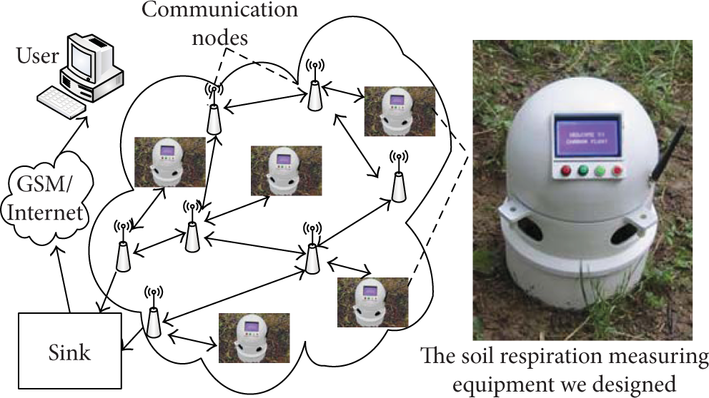
Wireless sensor network for soil respiration monitoring.

But we encountered a problem during the practical construction process of soil respiration monitoring sensor networks; that is, the number of soil respiration sensing nodes is limited due to the high cost, which makes a well-designed deployment strategy become an urgent need to use fewer nodes monitoring a target region.

Although there have been a lot of research works aimed at nodes deployment issues in wireless sensor networks, most of them are to study the coverage of monitoring area and network connectivity issues. Furthermore, most of these studies are generic methods to solve the deployment problem and not for a specific application scenario. However, there is usually some specific domain knowledge in the relevant fields of each practical application, and using such domain knowledge may lead to noneligible promoting effect on the solution to the deployment problem when wireless sensor network technology is applied in practical fields.

Because soil respiration in a position has an approximately day-periodic variation trend [5], the analyzing result of the former sensing data can play a guiding role for the later measurement. The diel variation trend of a position is affected by the environment parameters, so positions with similar parameters may have similar time domain features. It is very possible that some positions in a region with the same vegetation have similar parameters. As a result, if the initial measurement data of different positions have similar time domain features, the same similarity will be maintained in the process of subsequent measurement.

Therefore, we designed a deployment strategy of soil respiration sensor networks based on time domain feature similarity of lightweight parameters, TimSim. At first, according to the domain knowledge of soil respiration, the soil respiration is described by some lightweight parameters. Then positions are divided into groups according to time domain similarity of lightweight parameters, and positions in each group have similar trends of soil respiration. Then a representative position is chosen from each group, in which a soil respiration sensing node will be deployed. Because the time domain similarity exists, the soil respiration data of other positions in the same group can be obtained by a certain conversion of the soil respiration data from the deployed position. As a result, soil respiration data of the positions in the monitored region can be obtained by a small number of deployed nodes.

What should be emphasized is that although this method is put forward for a specific application of soil respiration monitoring, in fact the idea has universality and can be used for other applications with lightweight parameters, in which the monitoring data is periodic and sensing nodes costs are high. Therefore, the presented method can provide reference for solving problems during the application of wireless sensor network technology to other fields and promote wider application of wireless sensor networks.

The remaining parts of this paper are organized as follows. Section 2 introduces some previous work related to the subject this paper. Section 3 describes the nodes deployment problem in soil respiration monitoring sensor network to solve in this paper. Section 4 introduces in detail the proposed deployment strategy of soil respiration measurement nodes based on time domain similarity of lightweight parameters, TimSim. Section 5 verifies the performance of TimSim by experiments and compared with other two deployment methods. Finally, Section 6 carries on the summary and conclusions of the full paper and discusses the directions for further research.

2. Related Work

2.1. Deployment of Wireless Sensor Networks

Wireless sensor network technology can be used for many applications such as industry automation, localization and track tracing, health monitoring, and environment monitoring. Deployment is an important and basic issue for each of such applications. The concerns of the deployment problem include coverage, connectivity, and energy-efficiency.

The coverage problem of a wireless sensor network for different applications includes field coverage and barrier coverage, and the field may be two-dimensional area or three-dimensional space or surface. The basic deployment method for 2D area coverage is cell-based, and the shape of each cell may be square, triangle, hexagon, and so on. Ammari and Das [6] studied the coverage and connectivity of wireless sensor networks in 3D space using integrated concentric sphere model and continuum percolation theory, so as to determine the critical density of sensor nodes for the deployment and topology control. Liu and Ma [7] analyzed the expected coverage ratios on both regular and irregular 3D surface using stochastic sensors deployment method. For barrier coverage, there are line-based model [8] and curve-based model [9] for the deployment of wireless sensor networks. Furthermore, the coverage requirement may be k-coverage for redundancy in some applications. Ammari and Das [10] studied the node space density required for full k-coverage in an area so as to guide the deployment of sensor nodes. Li et al. [11] proposed a field k-coverage autonomous deployment method when the count of nodes is not abundant with the consideration of load-balance, using the localization and mobility of nodes. Mahboubi et al. [12–14] studied the distributed deployment of mobile sensor networks using weighted Voronoi diagram model, in which nodes can move to sparse or empty area so as to fulfill better coverage.

The connectivity and energy-efficiency are also considered by many deployment methods besides coverage. If there are obstacles in the field, a serpentine movement policy can be used to handle obstacle [15]. The positions of relay nodes are important for the connectivity of a network. Lee and Younis [16] studied the selection and deployment problem of relay nodes, when some nodes failed and the network is separated into segments. The deployment of relay nodes can also be guided by the communication load of the network, so as to place more relay nodes in heavy load region [17]. Liu et al. [18] studied the deployment of sensor nodes using minimum cost when the required lifetime of network is given. Energy can also be saved through optimizing the distance of movement of sensor nodes in mobile sensor networks [19].

Compared with the previous work, the main novelty of TimSim lies in its different angle of view to solve the deployment problem of sensor nodes. These previous researches about the deployment of wireless sensor networks focusing on the coverage, connectivity, and energy-efficiency are on generic level and without specific application field. What we are considering in this paper is the utilization of domain knowledge of soil respiration, which is necessary and important.

2.2. Wireless Sensor Networks for Environment Monitoring

There are many systems using wireless sensor network technology in the recent years. Barrenetxea et al. [20] established a wireless sensor network system for wild environment monitoring. GreenOrbs is a wireless sensor network system in forest for canopy closure sustainable estimation [21]. Besides, wireless sensor network technology is also used for volcano monitoring [22], wildlife monitoring [23], marine environment monitoring [24], soil property monitoring [25], and so on. In these systems, the focus is the application rather than deployment, so they do not have particular design for the optimization of the count and positions of sensor nodes.

Some environment monitoring applications use graph theory to optimize the positions of sensor nodes [26, 27]. However, these graph-based methods are generic and do not utilize any knowledge of applications. Du et al. [28] introduced a wireless sensor network system for wind distribution monitoring around an urban reservoir, in which sparse deployment is accomplished by adjusting distance of communication. However, it did not introduce how to determine the positions of sensor nodes.

Du et al. [29] segmented a year into different monsoon seasons according to the analysis of historical wind distribution data of the field and used computational fluid dynamics to learn the spatial correlation of wind in the presence of surrounding buildings. The most informative locations are the outputs of the deployment method. This method uses knowledge of application, which is similar to our method. However it cannot be used in soil respiration monitoring sensor network, because we cannot have historical soil respiration data of a monitored field and computational fluid dynamics cannot be used for soil respiration.

As to the previous works, the deployment methods of them are all different from the method based on similarities of lightweight parameters, which is to be studied in this paper.

3. Problem Descriptions

3.1. Soil Respiration Sensor Network

In order to monitor soil respiration carbon flux data in a region, traditional methods are to carry out measurements in one or a few sampling positions using devices such as LI-8100 and then estimate soil respiration carbon fluxes across the region. But the results of such methods using a small number of measuring positions are very inaccurate. On the one hand, for the spatial heterogeneity of soil respiration, using a small amount of measuring positions to represent other positions in the region as a whole is not appropriate [30]; on the other hand, soil respiration varies over time and the result measured at a certain moment cannot represent the measurements of other moments [31]. So the traditional measuring methods are not representative in both time and space aspects, and regional soil respiration carbon flux cannot be accurately estimated using traditional methods.

Therefore accurate measurement and estimation of regional soil respiration should meet the following three requirements. (1) Measurements in multiple positions: due to the spatial heterogeneity of soil respiration, only measurement results of multiposition can describe the entire regional soil respiration accurately. (2) Measurements at the same time in multiple positions: because of the time heterogeneity of soil respiration, measurements in the same position at different time may be different, so only measurements at the same time in multiple positions can describe the regional soil respiration at the measuring time. (3) Continuous measurements: for the temporal heterogeneity of soil respiration, few measurements cannot reflect the details of the soil respiration varying with time, and only continuous measurements can reflect the varying details of soil respiration along with time.

Wireless sensor network technology can well meet the three aspects of requirements of measurements: multiple positions, synchronization, and continuation. So we adopt this technology to carry out the measurement and estimation of regional soil respiration carbon flux. During the construction of a soil respiration sensor network, because the soil respiration measuring equipment is expensive which leads to limited quantity of the equipment, we add some routing nodes which bear only communication tasks and are not responsible for the measurement task to guarantee the connectivity of the network, as shown in Figure 1. In order to save energy of these nodes, soil respiration measuring nodes act as leaf nods in the data collecting tree, and measured data will be transferred to the sink node by routing nodes. In addition, we have studied segmental dynamic sampling strategy to reduce energy consumption of soil respiration measuring nodes and prolong the continuous working time of the whole system in our previous study [32].

3.2. Deployment of Soil Respiration Sensing Nodes

As mentioned above, a soil respiration sensor network contains some routing nodes to guarantee the connectivity of the network, so the deployment positions of soil respiration nodes mainly consider the requirements of application layer rather than network layer. At the application layer, in order to effectively measure regional soil respiration using a limited number of soil respiration sensing nodes, each node should be deployed in a more reasonable position.

Deploying a soil respiration sensor network in the region Z, in addition to the sink node, there are N soil respiration sensing nodes $S=\{s_{\mathrm{1}},s_{\mathrm{2}},\dots ,s_N\}$ and some routing nodes R. Soil respiration nodes S are deployed in $P_s=\{p_{s_{\mathrm{1}}},p_{s_{\mathrm{2}}},\dots ,p_{s_N}\}$ , and $p_{s_i}=(x_i,y_i)$ , $(\mathrm{1}\le i\le N)$ represents the physical position where the soil respiration measuring node $s_i$ deploys. The number and positions of routing nodes R depend on the quantity and location of soil respiration nodes and are determined according to the connectivity and robustness requirements, which is not in the scope of this paper.

The goal of this paper is to determine small N and appropriate $P_s$ , according to which soil respiration sensing data $\text{SR}=\{\text{s}{\text{r}}_{\mathrm{1}},\text{s}{\text{r}}_{\mathrm{2}},\dots ,\text{s}{\text{r}}_N\}$ are obtained by sensing nodes $S=\{s_{\mathrm{1}},s_{\mathrm{2}},\dots ,s_N\}$ in the positions $P_s$ . The errors between spatial interpolation results $\text{S}{\text{R}}^{\prime }=\{\text{s}{\text{r}}_{\mathrm{1}},\text{s}{\text{r}}_{\mathrm{2}},\dots ,\text{s}{\text{r}}_N,\text{s}{\text{r}}_{N+\mathrm{1}},\text{s}{\text{r}}_{N+\mathrm{2}},\dots ,\text{s}{\text{r}}_{N^{\prime }}\}$ and the real soil respiration data in $N^{\prime }$ positions, $E=\{e_{\mathrm{1}},e_{\mathrm{2}},\dots ,e_N\}$ , are computed and small mean error and small error variance are preferred.

4. Our Solution

4.1. Main Idea

In order to solve the problem of reasonable layout of sampling positions, a relatively easy way is to arrange more sampling positions in subregions with more drastic changes of soil respiration so as to get more details of the changes and to choose fewer sampling positions in subregions with relatively flat changes of soil respiration. This approach is based on the spatial correlation of soil respiration, which means each measurement in a position represents the data in surrounding area, and the correlation can be exploited by spatial interpolation. As a result, the distribution state of sensing data in the entire region can be obtained by interpolation using a small number of measurement points.

The method above only pays attention to the local spatial correlation of soil respiration, the main consideration of which is the relationship of soil respiration of a position and that of positions nearby it. But the approach does not take into account the correlation between soil respiration of positions which are not adjacent. In addition to the correlation among adjacent positions which are naturally used in the spatial interpolation process, the correlation of soil respiration data measured in nonadjacent positions may play a significant role in promoting the rationality of the layout of soil respiration sensor network, which is the focus of this paper.

In this paper we designed a soil respiration nodes deployment method exploiting the correlation of soil respiration data in nonadjacent positions. According to the similarity of time domain features of soil respiration data in different positions of monitored area, these positions are divided into groups regardless of whether positions in each group are adjacent or not in physical space, and thus soil respiration data monitored in one position from each group can represent the remaining positions of the same group for the time domain similarity. During the monitoring stage, once soil respiration data are measured in the chosen sampling position of each group, soil respiration data of other positions in the same group can be obtained through certain transformation relations which are found during the grouping process. As a result, we can have soil respiration data of positions much more than sensing nodes actually deployed before final interpolation to simulate the real state of regional soil respiration, which makes the interpolation result closer to the real world.

However, obtaining the time domain similarities of soil respiration data of all positions in the monitored area is very difficult, since it needs fine-grained soil respiration data of each position in the monitored area for a period of time, which is the ultimate goal of soil respiration monitoring sensor network, and can only be realized through dense and regular deployment of soil respiration measuring nodes. In fact, it is not realistic to densely deploy soil respiration measuring nodes in the monitored area, because we cannot have enough soil respiration measuring nodes usually due to expensive cost, which is just the root cause of what to be studied in this paper.

To solve the problem above, we introduced the temporal similarity of lightweight parameters into the solution. According to the domain knowledge of soil respiration, soil respiration sensing nodes use open chamber method to measure the soil respiratory carbon flux, and the calculation is shown by [4]

$$\begin{array}{cc}& C_{\text{flux}}=\frac{\mathrm{100}V{P}_{\mathrm{0}}\left(\mathrm{1}-W_{\mathrm{0}}/\mathrm{1000}\right)}{rs\left(T_{\mathrm{0}}+\mathrm{273.15}\right)}\frac{\partial C^{\prime }}{\partial t}.\end{array}$$

(1)

In the equation, $C_{\text{flux}}$ means soil respiration carbon flux, V means chamber volume (cm³), $P_{\mathrm{0}}$ means initial pressure in the chamber (kPa), $W_{\mathrm{0}}$ means initial water vapor mole fraction (mmol·mol⁻¹), r means ideal gas constant 8.314472 m³·Pa·mol⁻¹·K⁻¹, s means soil surface area (cm²), $T_{\mathrm{0}}$ means initial temperature (°C), and $\partial C^{\prime }/\partial t$ means initial changing rate of CO₂ (mol·m⁻²·s⁻¹).

From (1) we can see that soil respiration is affected by temperature, humidity, pressure, and other factors. Because price and energy consumption of sensors for these parameters are relatively low, we refer to these factors such as temperature, humidity, and pressure as “lightweight parameters” of soil respiration in this paper.

In order to solve the problem that the similarities of time domain features of fine-grained positional soil respiration data in the monitored area cannot be obtained directly, we converted the similarities into the similarities of time domain features of lightweight parameters in different positions. Because of the low cost and low energy consumption of lightweight parameter sensing nodes, lightweight parameters can be measured densely and regularly in the monitored area and the similarities of time domain features of lightweight parameters in different positions can be obtained.

Therefore, we prposed a strategy for the deployment of soil respiration monitoring sensor network based on similarity of time domain features of lightweight parameters, which is called TimSim in this paper. Firstly densely and regularly deploy lightweight parameters sensing nodes in the monitored area and measure for a period of time, and then analyze the measurement results to observe the similarities of time domain features of lightweight parameters, group the positions according to the similarities, and finally choose a representative position for each group to deploy a soil respiration measurement node.

What should be emphasized is that because deploying a soil respiration measuring node requires some complicated special processes such as smoothing the ground surface and embedding the device bottom into the soil, once the layout scheme of sensor nodes is determined, it is usually assumed that soil respiration sensing nodes in the monitoring period will not be moved anymore after deployment. Therefore, these complex preparatory works including the measurement, analysis, and computation of lightweight parameters are very necessary for the optimal layout scheme of sensor nodes.

4.2. Temporal Similarity of Data in Different Positions

In order to group similar positions in the monitored area using the time domain features of the data, the similarity of time domain features of data between different positions need be defined.

Let $D_p=\{d_{p_i}\hspace{0.17em}|\hspace{0.17em}\mathrm{1}\le i\le l\}$ and $D_q=\{d_{q_i}\parallel \mathrm{1}\le i\le l\}$ denote two time series of data measured in positions p and q, respectively, in which l means the length of the data series. In order to describe the similarity between $D_p$ and $D_q$ , they are regarded as the two l dimensional vectors, and then the cosine value of angle θ between these two l dimensional vectors can be used as the similarity metrics. So we define the temporal similarity of data in the two positions of the p and q, $\text{Sim}(p,q)$ , as

$$\begin{array}{l}\text{Sim}\left(p,q\right)=\cos \left(\theta \right)=\frac{D_p·D_q}{‖D_p‖‖D_q‖}\\ =\frac{{\sum }_{i=\mathrm{1}}^l\left(d_{p_i}\times d_{q_i}\right)}{\sqrt{{\sum }_{i=\mathrm{1}}^l{d}_{p_i}^{\mathrm{2}}}\times \sqrt{{\sum }_{i=\mathrm{1}}^l{d}_{q_i}^{\mathrm{2}}}}.\end{array}$$

(2)

Because all the data in this application, either soil respiration data or lightweight parameters data, are all positive, the components of $D_p$ and $D_q$ are not negative, and hence the value of $\text{Sim}(p,q)$ is in the zone $[\mathrm{0,1}]$ . Obviously, if the directions of $D_p$ and $D_q$ are identical, that is, there exists the same linear relationship between $D_p$ and $D_q$ components, the similarity between $D_p$ and $D_q$ is the best, and $\text{Sim}(p,q)$ equals 1. On the contrary, if the two vectors, $D_p$ and $D_q$ , are orthogonal to each other, the similarity is minimum and $\text{Sim}(p,q)$ equals 0.

4.3. Grouping Positions according to Temporal Similarity

After the temporal similarity of data between two positions is defined, we can divide multiple positions into different groups according to the similarities between each other, and the grouping result is that positions in each group have high similarities of time domain features of data while there are less similarities among positions from different groups. There are two cases about the grouping problem in practice, one of which is that the number of groups, k, is determined and the other is that the lower bound of similarity among positions in the same group, $\text{L}{\text{B}}_{\text{Sim}}$ , is given.

When the number of groups k is identified, which means the count of soil respiration sensing nodes is limited, we can use clustering algorithms based on partition, for example, k-means, to divide n positions $P=\{p_i\hspace{0.17em}|\hspace{0.17em}\mathrm{1}\le i\le n\}$ into k groups $G=\{g_i\hspace{0.17em}|\hspace{0.17em}\mathrm{1}\le i\le k\}$ . The stop condition of clustering procedure is that the differences among average similarities of positions in every group $g_i\mathrm{\hspace{0.17em}\hspace{0.17em}}(\mathrm{1}\le i\le k)$ are below a preset threshold. Obviously, the bigger the k is, the more the groups are divided, the fewer the positions are in a group, the smaller the ${\theta }_i$ is, and the higher the similarities among positions in a group are.

When the lower bound of group similarity $\text{L}{\text{B}}_{\text{Sim}}$ is given, which means the count of soil respiration sensing nodes is relatively abound and what we are pursuing is the accuracy of results, we can use clustering algorithm based on hierarchy, such as ROCK [33], to divide n positions $P=\{p_i\hspace{0.17em}|\hspace{0.17em}\mathrm{1}\le i\le n\}$ into $k^{\prime }$ groups $G^{\prime }=\{g_i\hspace{0.17em}|\hspace{0.17em}\mathrm{1}\le i\le k^{\prime }\}$ . Minimum similarity in each group $g_i\mathrm{\hspace{0.17em}\hspace{0.17em}}(\mathrm{1}\le i\le k^{\prime })$ , $\text{Si}{\text{m}}_i$ , is bigger than the preset similarity threshold $\text{L}{\text{B}}_{\text{Sim}}$ . Obviously, the bigger the $\text{L}{\text{B}}_{\text{Sim}}$ is, the higher the similarities of positions in each group are, the fewer the positions are in a group, the more the group number $k^{\prime }$ is, and the more the sensing nodes are needed.

After the grouping scheme of positions in the monitored area is determined and the grouping result is achieved, we choose the position where the data vector has the highest similarity with the center vector of all data vectors in the same group as the position to deploy a soil respiration sensing node. When the deploying positions in all groups are chosen, the positions of routing nodes R can be determined according to the connectivity requirement of soil respiration sensing nodes.

One position in each group is selected as a representative for the soil respiration sampling. Therefore, if the number of soil respiration measuring nodes to deploy is certain, we use the case of determined k, the number of groups. Otherwise, the situation is corresponding to the case of similarity lower bound $\text{L}{\text{B}}_{\text{Sim}}$ which is identified. Higher $\text{L}{\text{B}}_{\text{Sim}}$ leads to not only higher monitored accuracy of regional soil respiration, but also bigger group count $k^{\prime }$ which needs more soil respiration sensing nodes, that is, higher network cost, so an appropriate $\text{L}{\text{B}}_{\text{Sim}}$ should keep a compromise between accuracy of results and cost of network.

4.4. Reconstruction of Data for Positions of a Group

A following problem is the reconstruction of data for the rest of positions using the data of the sampling position in a group. Data reconstruction should be done after the deployment and during the working stage of soil respiration sensor network system, and it seems that this issue is not a part of the deployment of a soil respiration sensor network. But in fact, as for the proposed deployment strategy based on time domain similarity of data, its main idea is taking advantage of the correlation of data from nonadjacent positions, so we should clarify that the method is able to rebuild the same correlation in data before putting the deployment strategy into practice. If the data correlation among nonadjacent positions used by the deployment strategy cannot be reconstructed during the network works, this deployment method will be not able to be applied into any applications.

The reconstruction problem of data of each position in a group is described as follows. Assume that a position group g contains m positions $P_g=\{p_i\hspace{0.17em}|\hspace{0.17em}\mathrm{1}\le i\le m\}$ and the sampling position in the group is $gc$ , $(gc\in P_g)$ , whose data vector is the closest to the centroid of vectors of all group member positions in the grouping result. Before the grouping process, the temporal data sequence measured in position $p_i$ is $D_{p_i}=\{d_{p_{i}j}\hspace{0.17em}|\hspace{0.17em}\mathrm{1}\le i\le m,\mathrm{1}\le j\le l\}$ and data sequence measured in position $gc$ is $D_{gc}=\{d_{g{c}_i}\hspace{0.17em}|\hspace{0.17em}\mathrm{1}\le i\le l\}$ . After the deployment of whole sensor network (i.e., only in position $gc$ a soil respiration sensing node is deployed in this group), we obtain data $d_{gc}^{\prime }$ measured in position $gc$ . The data reconstruction problem we need solve is how to build data for the rest of $m-\mathrm{1}$ positions in group g using the data $d_{gc}^{\prime }$ .

To fulfill this task, we need compute and save the conversion relations between the data vectors of the rest of $m-\mathrm{1}$ positions in the group and that of $gc$ during the grouping procedure. These positions are grouped into a group because the similarities of temporal features of data vectors in these positions are high; that is, the directions of the data vectors are closer and can be considered as the same direction approximately, which means that the ratio relationships among data of these positions at the same time remain still. The norm of data vector of position $p_i$ is $‖D_{p_i}‖$ and that of $gc$ is $‖D_{gc}‖$ . If we calculate and save the ratio between these two norms $\text{rati}{\text{o}}_i=‖D_{p_i}‖/‖D_{gc}‖$ , the data of position $p_i$ at the same time to time $d_{gc}^{\prime }$ was measured in position $gc$ , $d_{p_i}^{\prime }$ , can be estimated by $d_{p_i}^{\prime }=d_{gc}^{\prime }\times \text{rati}{\text{o}}_i$ .

During the analysis of premeasured data for grouping, record the ratios Ratio between data vector of every nodes $p_i$ in group $P_g$ and that of sampling position $gc$ :

$$\begin{array}{cc}& \text{Ratio}=\left\{\text{rati}{\text{o}}_i\right\}=\left\{\frac{‖D_{p_i}‖}{‖D_{gc}‖}\right\},\mathrm{1}\le i\le m.\end{array}$$

(3)

Then data of all positions in the group can be reconstructed using Ratio after data $d_{gc}$ are measured in position $gc$ after the soil respiration measuring node is deployed in position $gc$ and during the persistent practical monitoring procedure:

$$\begin{array}{cc}& D_{p_g}^{\prime }=\left\{d_{p_i}^{\prime }\right\}=\text{Ratio}·‖d_{gc}^{\prime }‖,\mathrm{1}\le i\le m.\end{array}$$

(4)

But in the approach we designed in this paper, the premeasured data is lightweight parameters data rather than soil respiration data, and the ratio vector Ratio is the relation of lightweight parameters data of each position within the group rather than that of soil respiration data. So this ratio vector Ratio can only be used to reconstruct lightweight parameters data and cannot be directly used for the reconstruction of soil respiration data.

Because the soil respiration carbon flux is calculated according to (1), the lightweight parameters such as temperature and humidity measured in position $pc$ by the soil respiration sensing device can be used to calculate the soil respiration carbon flux on the one hand; on the other hand, these lightweight parameters data in position $pc$ can be used to get lightweight parameters data in other positions of the same group using (4), and then the soil respiration data in these positions can be calculated according to (1).

4.5. TimSim Algorithm

Now we formally describe the deployment strategy for soil respiration monitoring sensor network based on time domain similarity of lightweight parameters, TimSim, proposed in this paper.

Algorithm 1 requires the following: P: positions uniformly and densely distributed in the monitored area; $D_P$ : lightweight parameters data serials in these positions P; k or $\text{L}{\text{B}}_{\text{Sim}}$ : limiting conditions required for grouping in two cases, k for count limit of groups and $\text{L}{\text{B}}_{\text{Sim}}$ for lower bound of similarity in groups. In the process of the algorithm, firstly, outliers in data are rectified and other preprocessing operations are done, and then similarities of temporal features of every two data sequences in different positions are calculated. In the grouping process, positions in P are divided into k groups using k-means algorithm if parameter k is provided or divided into $k^{\prime }$ groups using ROCK algorithm if parameter $\text{L}{\text{B}}_{\text{Sim}}$ is provided. For each group of positions, the centroid vector of lightweight parameters data vectors is calculated, and choose the position where lightweight parameters’ data is the closest to the centroid vector as the representative position of the group, $g{c}_i$ , and then the ratios between data vectors in every other position and data vector in the representative position, $g\text{rati}{\text{o}}_i$ , are calculated and recorded for the data reconstruction of subsequent monitoring process later.

Algorithm 1: Time domain similarity of lightweight parameters based deployment algorithm (TimSim).

Require:  $$P=\{p_i\hspace{0.17em}|\hspace{0.17em}\mathrm{1}\le i\le n\}$$ // n positions regularly and densely distributed in the monitored area.

   $$D_P=\{D_{p_i}\hspace{0.17em}|\hspace{0.17em}\mathrm{1}\le i\le n\}=\{\{d_{p_{ij}}\hspace{0.17em}|\hspace{0.17em}\mathrm{1}\le j\le l\}\hspace{0.17em}|\hspace{0.17em}\mathrm{1}\le i\le n\}$$ // lightweight data sequence from each position

  k // limited number of soil respiration sensing nodes

   $$\text{L}{\text{B}}_{\text{Sim}}$$ // limited lower bound of similarity in each group

Ensure:  $$G=\{g_i\hspace{0.17em}|\hspace{0.17em}\cup \hspace{0.17em}{g}_i=P,\cap \hspace{0.17em}{g}_i=\mathrm{\varnothing },\mathrm{1}\le i\le k$$ (or $$k^{\prime })\}$$ // result of positions group

   $$GC=\{g{c}_i\hspace{0.17em}|\hspace{0.17em}g{c}_i\in g_i,\mathrm{1}\le i\le k$$ (or $$k^{\prime })\}$$ // $$g{c}_i$$ is the position to place a node in group $$g_i$$

   $$\text{Ratio}=\{g\text{rati}{\text{o}}_i=\{\text{rati}{\text{o}}_j\hspace{0.17em}|\hspace{0.17em}{p}_j\in g_i\}\hspace{0.17em}|\hspace{0.17em}\mathrm{1}\le i\le k$$ (or $$k^{\prime })\}$$ // data ratio between positions to node position

( $$\mathit{1}$$ )  preprocess( $$D_P$$ ); // rectify the outlier in data

( $$\mathit{2}$$ )  for  $$i=\mathrm{1}$$ to n  do

( $$\mathit{3}$$ )   for  $$j=\mathrm{1}$$ to n  do

( $$\mathit{4}$$ )     $$\text{Sim}(p_i,p_j)=\left(D_{p_i}·D_{p_j}\right)/\left(‖D_{p_i}‖‖D_{p_j}‖\right)$$ ;

( $$\mathit{5}$$ )   end for

( $$\mathit{6}$$ )  end for

( $$\mathit{7}$$ )   $$G=\{g_i\hspace{0.17em}|\hspace{0.17em}\mathrm{1}\le i\le k\}=k$$ -means $$(P,\text{Sim},k)$$ ; // for the case of k is given

  or $$G=\{g_i\hspace{0.17em}|\hspace{0.17em}\mathrm{1}\le i\le k^{\prime }\}=ROCK(P,\text{Sim},\text{L}{\text{B}}_{\text{Sim}})$$ ; // for the case of $$\text{L}{\text{B}}_{\text{Sim}}$$ is given

( $$\mathit{8}$$ )  for  $$i=\mathrm{1}$$ to k (or $$k^{\prime }$$ ) do

( $$\mathit{9}$$ )    $$D{c}_i$$ = centroid( $$\{D_{p_j}\hspace{0.17em}|\hspace{0.17em}{p}_j\in g_i,\cup \hspace{0.17em}\{p_j\}=g_i\}$$ ); // centroid of data vectors from all positions in $$g_i$$

( $$\mathit{10}$$ )    $$\text{Dis}{\text{t}}_i=\{\text{dis}{\text{t}}_j=\mathrm{1}/\text{Sim}(D_{p_j},D{c}_i)\hspace{0.17em}|\hspace{0.17em}{p}_j\in g_i,\cup \hspace{0.17em}\{p_j\}=g_i)\}$$ ; // distance to centroid data vector

( $$\mathit{11}$$ )    $$g{c}_i=\{p_j\hspace{0.17em}|\hspace{0.17em}\text{dis}{\text{t}}_j==\text{MIN}(\{\text{Dis}{\text{t}}_i\}),p_j\in g_i\}$$ ; // position with nearest data vector to centroid

( $$\mathit{12}$$ )    $$g\text{rati}{\text{o}}_i=\left\{‖D_{p_j}‖/‖D_{g{c}_i}‖\left|p_j\in gi,\cup \hspace{0.17em}\left\{p_j\right\}=g_i)\right.\right\}$$ ;

( $$\mathit{13}$$ )  end for

( $$\mathit{14}$$ )  return  $$G,GC=\{g{c}_i\},\text{Ratio}=\{g\text{rati}{\text{o}}_i\}$$ ;

As for the soil respiration sensing network, the length of time lightweight parameter data sequence $D_P$ covered is usually 24 hours, considering the soil respiration has day-periodic trends. Furthermore, to avoid the occasionality of data sequence, several data sequences of different days should be used as the basis of grouping operation after computing the average data sequence with time-correspondence.

5. Experiments and Analysis

5.1. Experimental Data

In order to verify the proposed deployment strategy of soil respiration monitoring sensor network based on similarity of time domain features of lightweight parameters, TimSim, the ideal experiment procedure should be as follows: densely and regularly deploy lightweight parameters sensing nodes in the monitored area Z and carry out a few days of continuous measurement, and then divide the positions into groups based on the lightweight parameters data sequences measured, and find the positions closest to the centroid of light weight data sequences to deploy soil respiration sensing nodes. In order to examine the performance of this method, we need collect soil respiration data in positions where soil respiration sensing nodes deployed and then do spatial interpolation with them to estimate regional soil respiration of the monitored area, $\text{S}{\text{R}}_{TimSim}$ . The estimated results should be compared with the real soil respiration data $\text{S}{\text{R}}_{\text{real}}$ of the monitored area at the same time to analyze the measuring error of the method. But the real soil respiration data of the area, $\text{S}{\text{R}}_{\text{real}}$ , cannot be obtained, because this requires to deploy many soil respiration measuring equipments very densely throughout the area, while we cannot have so many soil respiration measuring equipments for the high cost.

We adopt a substitutional method to simulate real soil respiration data of many dense positions in the monitored area using temporal and spatial shift. We deploy x soil respiration sensing nodes in x different positions of the experimental area and let them keep working for d days to obtain data of soil respiration and lightweight parameters. Thus d serials of daily soil respiration data can be collected by the equipment in each position in the d days. We shift the d daily serials of data of a position to d different positions for one day. So in order to simulate real data of one day in n positions of the experimental area, $\text{S}{\text{R}}_{\text{real}}$ , such x equipment need keep working for $n/x$ days.

Taking into account that there are several factors affecting soil respiration such as temperature, humidity, and air pressure, too many lightweight parameters may complicate the experiment. We carry out the experiment process in smooth lawn with uniform illumination, in which the temperature and pressure of different positions are almost the same; thus humidity is the only main factor affecting soil respiration in this area. So the lightweight parameter in our experiment only remains humidity data.

In the experiment, we used 20 soil respiration measuring equipments, deployed them in different positions of the monitored area, let them keep working for 5 days, and obtained 100 position-day serials of data. Then we changed the positions of such equipment and repeated the data collection process for 2 times. As a result, we obtained 3 data sets, each of which includes 100 position-day serials of data, and we distributed each data set regularly with $\mathrm{10}\times \mathrm{10}$ grids pattern in the monitored area as a set of experimental data, $\text{S}{\text{R}}_{\text{real}}$ .

5.2. Experimental Scheme

Suppose that we have measured regional soil respiration real data $\text{S}{\text{R}}_{\text{real}}$ ; then we can evaluate a specific deployment strategy using the deviation of $\text{S}{\text{R}}_{\text{strategy}}$ , the measured results of soil respiration data using the strategy, from $\text{S}{\text{R}}_{\text{real}}$ at each position $p_i$ :

$$\begin{array}{cc}& E=\left\{e_i\right\}=\left\{\left|\text{S}{{\text{R}}_{\text{strategy}}}_{p_i}-\text{S}{{\text{R}}_{\text{real}}}_{p_i}\right|\hspace{0.17em}|\hspace{0.17em}\mathrm{1}\le i\le n\right\}.\end{array}$$

(5)

Once we get the error between $\text{S}{\text{R}}_{\text{strategy}}$ and $\text{S}{\text{R}}_{\text{real}}$ , $e_i$ , in position $p_i$ , we can use mean error and error variance to analyze the performance of a deployment strategy. The mean error indicates an overall performance of a deployment scheme, and the error variance is helpful to analyze whether the errors of the different positions are close and to analyze the spatial distribution of error combining $e_i$ and the location of $p_i$ . Of course we expect that our method, TimSim, may have small mean error and small error variance.

In order to evaluate the performance of TimSim, we use the scheme in Algorithm 2 to carry out the experiment. As shown in Algorithm 2, we use multiple sets of the experimental data to calculate the error of regional soil respiration carbon flux measured using TimSim, Uniform, and Random deployment strategies.

Algorithm 2: Experiment procedure.

Require:  $$P=\{p_i\hspace{0.17em}|\hspace{0.17em}\mathrm{1}\le i\le n\}$$ // n positions regularly and densely distributed in the monitored area.

   $$D_P[\hspace{0.17em}]=\{\{D_{p_i}=\{d_{p_{ij}}\hspace{0.17em}|\hspace{0.17em}\mathrm{1}\le j\le l\}\hspace{0.17em}|\hspace{0.17em}\mathrm{1}\le i\le n{\}}_t\hspace{0.17em}|\hspace{0.17em}\mathrm{1}\le t\le \text{times}\}$$ // $$times$$ sets of lightweight data sequences of all positions

   $$\text{S}{\text{R}}_{\text{real}}[\hspace{0.17em}]=\{\{\text{s}{\text{r}}_{\text{rea}{\text{l}}_{\text{i}}}\hspace{0.17em}|\hspace{0.17em}\mathrm{1}\le i\le n{\}}_t\hspace{0.17em}|\hspace{0.17em}\mathrm{1}\le t\le \text{times}\}$$ // $$times$$ sets of data for experiment

Ensure:  $$\text{Err}[\hspace{0.17em}]$$ // error for each strategy.

( $$\mathit{1}$$ )   $$\text{times}=\mathrm{3},n=\mathrm{100},N_S=\{\mathrm{6,9},\mathrm{12,15}\}$$ ; // Initialization

( $$\mathit{2}$$ )   $$\text{STRATEGY}=$$ {TimSim, Uniform, Random}; // using three strategies respectively

( $$\mathit{3}$$ )  for each $$\text{strategy}\in \text{STRATEGY}$$   do

( $$\mathit{4}$$ )   for each $$n_s\in N_S$$   do

( $$\mathit{5}$$ )    for  $$t=\mathrm{1}$$ to $$\text{times}$$   do

( $$\mathit{6}$$ )      $$P_{\text{sample}}=\text{strategy}(P,D_P[t])=\{p_i\hspace{0.17em}|\hspace{0.17em}\mathrm{1}\le i\le n_s\}$$ ; // determining $$n_s$$ sample positions using $$\text{strategy}$$

( $$\mathit{7}$$ )      $$\text{S}{\text{R}}_{\text{sample}}=$$ sample $$(\text{S}{\text{R}}_{\text{real}}[t],P_{\text{sample}})=\{\text{s}{\text{r}}_{p_i}\hspace{0.17em}|\hspace{0.17em}{p}_i\in P_{\text{sample}},\mathrm{1}\le i\le n_s\}$$ ; // sampling $$n_s$$ data from $$\text{S}{\text{R}}_{\text{real}}[t]$$

     according to $$P_{\text{sample}}$$

( $$\mathit{8}$$ )      $$\text{S}{\text{R}}_{\text{strategy}}=\{\text{s}{\text{r}}_{p_i}\hspace{0.17em}|\hspace{0.17em}\mathrm{1}\le i\le n\}=$$ Kriging( $$\text{S}{\text{R}}_{\text{sample}},P_{\text{sample}},P$$ ) // interpolation using Kriging method

( $$\mathit{9}$$ )      $$E\left[\text{strategy},n_s,t\right]=\left\{e_i\hspace{0.17em}|\hspace{0.17em}\mathrm{1}\le i\le n\right\}=\left|\text{S}{\text{R}}_{\text{strategy}}-\text{S}{\text{R}}_{\text{real}}\left[t\right]\right|$$

( $$\mathit{10}$$ )   end for

( $$\mathit{11}$$ )  end for

( $$\mathit{12}$$ )   $$\text{Err}\left[\text{strategy},n_s\right]=\left(\mathrm{1}/\text{times}\right){{\displaystyle \sum }}_{t=\mathrm{1}}^{\text{times}}E\left[\text{stragegy},n_s,t\right]$$ ;

( $$\mathit{13}$$ )  end for

( $$\mathit{14}$$ )  return  $$\text{Err}$$ ;

5.3. Experimental Results and Analysis

5.3.1. Deployment Results and Performance Analysis of TimSim

In order to demonstrate the procedure and result of TimSim deployment method, we choose a set of experimental data, including lightweight parameter data, humidity, and soil respiration carbon flux data of 100 positions, and the data distribution of these positions at a moment is shown in Figure 2.

Figure 2

Distribution of soil humidity and soil respiration carbon flux in the experimental area.

Then the similarities of time domain features of lightweight parameter data are calculated using the data set, according to which the 100 positions are divided into groups using k-means algorithm. Figure 3 shows the grouping results of k-means algorithm for the case when the count k of groups is 6, 9, 12, and 15, respectively, in which positions marked with the same number are in the same group. Furthermore, the position to deploy a soil respiration sensing node in each group is marked with a small square around the number, whose data vector of lightweight parameter is the closest to the centroid of data vectors of all positions in the same group.

Figure 3

Position grouping results for different group numbers.

As we can see from Figure 3, there is not any obvious regular pattern in the spatial distribution of positions in each group. Positions in each group are not all adjacent in the space and their distribution is very disperse and irregular. When comparing the lightweight parameter data of positions in the same group, their values are not very close to each other at the same time. This is because the grouping method is based on the similarities of temporal pattern of data rather than the distribution of data at a certain moment.

As we can also see from Figure 3, the selected deployment positions of soil respiration sensing nodes are not in the geographical central positions of each group, because in our TimSim method the deployment position is determined by the centroid direction of data sequences in positions of a group, and the selected position to deploy soil respiration sensing node is the position whose direction of data vector is the closest to the centroid direction among all directions of data vectors in positions of the same group. So the selected deployment position is independent of the geographical distribution of positions of the same group.

After the deployment positions are determined, the distribution of error between $\text{S}{\text{R}}_{TimSim}$ and $\text{S}{\text{R}}_{\text{real}}$ can be obtained, which are shown in Figure 4. Figure 4 shows the distribution of average value of errors in each position using $\text{S}{\text{R}}_{TimSim}$ method for 3 times, as described in Algorithm 2, when group number k is 6, 9, 12, and 15, respectively. And the mean errors and error variances of all these cases are shown in Figure 5.

Figure 4

Error distribution of TimSim for different group numbers.

Figure 5

Error comparison of three deployment strategies.

From Figure 4 we can see that errors vary within a wide range when the count of sampling positions is small and there are large errors in some positions. For example, the biggest error among all positions reaches 4.8 in Figure 4(a). The reason is that the group count is low, and there are weak similarities between data vectors of some positions and that of the deployment positions in the same group, which brings big errors during the reconstruction process of data in these positions with weak similarities according to centroid vector. For the same reason, the mean and variance of errors of different positions are also relatively big when the group count is low, as shown in Figure 5.

With the increase of the number of sampling positions, the mean and variance of the errors decrease, as shown in Figure 5. From Figure 4 we can see that errors of most positions decrease with increasing the number of sample points with also some exceptional positions, which is caused by the alternation of directions of centroid vectors with the change of count of groups. Grouping results alter with the growth of count of groups, which makes the data vectors of some positions farther from the centroid vector directions than the former case leading to bigger error in these positions. While with the growth of count of groups, quantity of positions within a group is reduced at large, the similarities in groups become better and there are no positions with very large error. As shown in Figure 4(d), the maximum error among all positions is only 0.9.

5.3.2. Comparison of TimSim and Other Methods

In order to show the advantage of the TimSim method, we also evaluate other two deployment strategies, uniform deployment (Uniform) and random deployment (Random), using the same experimental data in our experiment as described in Algorithm 2, as shown in Figure 5. The experimental results show that the performance of TimSim is better than those of the other two strategies.

As can be seen from Figure 5, when the number of sampling positions is low, the mean errors of Uniform deployment and TimSim deployment are close to each other and are 3.2 and 3, respectively, and both of them have significantly better performance than random deployment, whose mean error is 3.9. The reason is that both Uniform deployment and TimSim can make the sampling positions cover the entire area well through spatial interpolation, while the coverage of Random deployment strategy is seriously inadequate due to the small number of nodes, resulting in large errors in the positions of uncovered area.

In addition, the error variance of TimSim has obvious advantages compared to those of both Uniform and Random deployment strategies in the case of few sampling nodes and the reason is that TimSim strategy takes the correlation among nonadjacent positions into account, which makes no positions have too large error. The other two strategies use the spatial correlations of soil respiration during the interpolation operations while the correlations may be not the actual case, so there may be large local deviations in some positions where nodes are sparse, which makes the errors relatively dispersed and leads to large error variances.

When the count of sampling positions is high, TimSim deployment strategy has obvious advantage in the aspect of either mean error or error variance compared with Uniform and Random deployment. When the number of sampling positions is up to 15, the coverage of Random deployment increases and the mean error was about to catch up with the Uniform deployment while the error variance is relatively high due to the inhomogeneity of deployment positions.

With the increase of deployment positions, number of groups increases in the TimSim deployment method and number of positions included in each group is reduced, which makes the similarities of temporal features of lightweight parameters in positions of the same group become high. As a result, the data in positions can be reconstructed with small error using data in the deployment position, which means that real data measured in 15 positions can be extended to approximate real data far more than 15 positions, so both mean error and error variance of TimSim deployment method are smaller than the other two deployment methods when the number of sampling positions is large to a certain extent.

6. Conclusions

Focusing on the problem of limited number of nodes for its expensive cost in soil respiration sensor networks, we proposed a new deployment strategy based on the time domain similarity of lightweight parameters, TimSim. This method is inspired by the knowledge that soil respiration is mainly affected by some lightweight parameters such as temperature and humidity. Using this method, the count of sampling positions can be reduced while the accuracy of results remains by proper arrangement of the node positions. The performance of TimSim is examined by experiments, and the results show that TimSim can measure regional soil respiration carbon flux effectively and can achieve smaller deviation than uniform or random deployment when using the same amount of measuring equipment.

In the proposed method, lightweight parameters data need to be measured densely and regularly in advance, which is infeasible when the area to be monitored is very large. In this case lightweight parameters can be relatively sparsely measured and then be interpolated to increase the density. Although this can reduce the accuracy of the final result, it is a feasible way anyway.

The method proposed in this paper is more convenient to be used for single factor than multiple factors of lightweight parameters, and the experiment in the paper also emphasized the guidance of a single lightweight parameter, humidity, to the deployment of soil respiration sensing nodes. When there are multiple factors, the problem is that the grouping results may be different using different lightweight parameters. A possible solution is to fuse multiple lightweight parameters as a complex lightweight parameter and analyze its temporal similarities among different positions using TimSim deployment strategy and the detailed solution to this problem is a direction we will study in future.

Finally, although the proposed deployment method based on lightweight parameters in this paper is described as a solution to soil respiration sensor networks, this idea for deployment is applicable and can provide a reference and guidance to other applications of wireless sensor networks.