Sage Journals: Discover world-class research

Abstract

Real-time traffic speed is indispensable for many ITS applications, such as traffic-aware route planning and eco-driving advisory system. Existing traffic speed estimation solutions assume vehicles travel along roads using constant speed. However, this assumption does not hold due to traffic dynamicity and can potentially lead to inaccurate estimation in real world. In this paper, we propose a novel in-network traffic speed estimation approach using infrastructure-free vehicular networks. The proposed solution utilizes macroscopic traffic flow model to estimate the traffic condition. The selected model only relies on vehicle density, which is less likely to be affected by the traffic dynamicity. In addition, we also demonstrate an application of the proposed solution in real-time route planning applications. Extensive evaluations using both traffic trace based large scale simulation and testbed based implementation have been performed. The results show that our solution outperforms some existing ones in terms of accuracy and efficiency in traffic-aware route planning applications.

1. Introduction

Nowadays, public traffic is a serious problem in big cities. Billions of hours are wasted everyday on traffic congestions. In addition, emission caused by vehicles has become one of the major sources of air pollution. To tackle these problems, people have developed many intelligent transportation system (ITS) applications to reduce vehicle traveling time by route planning [1] and to reduce emission by driving advisory [2]. To develop such ITS applications, real-time traffic information is a key prerequisite. With accurate real-time traffic information as prior knowledge, the performance of route planning and emission reduction can be significantly improved.

How to obtain real-time traffic information is one of the major issues to be solved. Conventional methods leverage traffic monitoring infrastructures, such as video surveillance cameras [3], inductive loops [4], or the combination of them to collect traffic data [5]. The main problem of this approach is the low availability of these facilities, due to the high deployment and maintenance cost. One alternative approach is to analyze historical traffic data [6] to find out some statistical traffic patterns. Unfortunately, historical data can not always reflect current situation since many emergent events (e.g., traffic accident) or temporary events (e.g. road surface maintenance) can lead to significant traffic flow variation.

Recently, using vehicular crowdsourcing to collect floating car data (FCD) for speed estimation [7] has attracted the attention of both academic and industrial bodies. Compared with infrastructure based approaches, the data collection cost of crowdsourcing is significantly reduced by leveraging individual users' contribution. However, the data transmission cost is still considerably high due to the use of cellular data to collect FCD for centralized data processing. In many ITS applications (e.g., route planning), the real-time traffic information of a road segment is only interested by the nearby vehicles. In these scenarios, an in-network traffic speed estimation solution is especially promising. Moreover, in-network processing can also reduce the cost of long distance data transmission.

With the rapid advancement of wireless communication and embedded technology, using vehicular ad hoc networks (VANET) to collect traffic information becomes popular recently [8–11]. Traffic information can be collected through vehicle to infrastructure (V2I) or vehicle to vehicle (V2V) communication. However, it is not easy to collect floating car data using VANETs. Considering the unique characteristics of VANETs and the application scenario, several challenging issues are raised: (i)

Network Disconnection. Vehicle mobility is highly dynamic, which can cause the network to be frequently disconnected. When using VANET to collect traffic information, an interesting contradiction can be found between traffic condition and network condition. Good traffic condition (high vehicle speed, low traffic density) usually leads to poor network condition (high packet loss, opportunistic network) and vice versa. The solution must tolerate the poor network conditions.

(ii)

Vehicle Speed Variation. Vehicles on roads do not travel using constant speed. The individual vehicle speed can have remarkable change in a short period. For example, a red light is in front, or a taxi stops at the request of passengers. The instant variation of floating car data can lead to inaccuracy to the traffic estimation algorithm. A good analysis model must be able to eliminate this variation.

(iii)

Insufficient Traffic Sampling. Due to the infrastructure-less nature of VANETs, it is not easy to monitor an area for a long period of time. Moreover, the fast-changing individual vehicle speed and fragile network topology can potentially interfere with the data collection. Hence, the data sampling is always insufficient. The traffic estimation algorithm needs to deal with insufficient traffic sampling condition.

To tackle these challenges, some infrastructure based solution has been proposed. These solutions utilize roadside unit (e.g., Wi-Fi access points [12], cellular base stations [13], etc.) and vehicle to infrastructure (V2I) communication to monitor the traffic condition of a fixed area. With the help of roadside infrastructure, continuous sampling of an area and caching collected data can easily be achieved. However, these solutions have the same deployment problem as those traffic facility based solutions. Other researches rely on the assumption that vehicles travel with constant speed [8, 14]. Without considering vehicle speed variation, some straightforward traffic estimation algorithms like time mean speed or space mean speed can be developed. However, this assumption does not hold in real world and it can lead to inaccurate traffic speed estimation results.

In this paper, we propose a novel in-network traffic information collection and estimation solution. We name it MICE or Model based Infrastructure-free traffic Collection and Estimation. In MICE, traffic information is collected using infrastructure-free approach. Then, traffic condition is estimated using in-network data processing and macroscopic traffic flow model. The application scenario is depicted in Figure 1. When a vehicle wants to know the traffic condition of nearby roads, it sends a traffic collection request using V2V communication to ambient vehicles on demand. Those vehicles that received the request send their information back to the original vehicle for traffic condition estimation.

Figure 1

Application scenario and system model: using V2V communication to collect real-time traffic information.

The contributions of this work can be summarized as follows: (1)

We propose a floating car data collection protocol, which leverages V2V communication. It can collect floating car data in segment level granularity and it is adaptive to different network conditions.

(2)

We adopt Underwood density-speed traffic flow model [15] developed by traffic scientists to predict the traffic speed. This model can eliminate the temporary speed variations to improve the estimation accuracy, efficient enough for in-network data processing.

(3)

We apply the proposed solution to the shortest-time route planning application. A heuristic based path finding algorithm is proposed to show how the proposed solution works in real world applications.

(4)

Extensive evaluations and analysis are conducted using both large scale simulation and testbed implementation. Evaluation results show that our solution outperforms some static and dynamic route planning solutions.

The remainder of this paper is organized as follows: related works are summarized in Section 2. The MICE problem is formulated in Section 3. The solution to MICE is presented in Section 4 in detail. In Section 5, an application of the proposed solution is introduced. The evaluations and results will be analyzed in Section 6. Finally, Section 7 concludes this paper.

2. Related Work

Several related works on using VANET to estimate traffic speed can be found in literature. We first introduce the works on traffic information collection, followed by existing traffic speed estimation solutions.

2.1. Traffic Information Collection

Solutions on traffic information collection can be classified by whether they rely on road side infrastructure. Road side infrastructure can simplify network protocol design since it is a convenient place to store, cache, and analyze data. Many infrastructure based solutions have been proposed [9, 10, 16, 17].

PeerTIS and Kyun queue are two typical infrastructure based solutions. PeerTIS [13] firstly constructs a peer to peer overlay using cellular networks among vehicles. A traffic information dissemination protocol is developed to share information among vehicles. The drawbacks of using cellular networks as infrastructures are the high communication cost. Kyun queue [18] proposed a novel solution to use RSSI to monitor the road traffic congestion. Specifically, it monitors the length of the waiting queue in front of a road intersection by observing the interference caused by stopping cars. The proposed solution is simple and yet effective. However, road side wireless nodes still need to be deployed as infrastructures in advance.

Infrastructure-free solutions only use communication among vehicles and no extra infrastructure needs to be deployed. Therefore, it is more flexible [8, 19]. MobSampling, Geocache, and V2R2 are three typical solutions of this type.

PGB [20] is an infrastructure-free data collection solution. The key idea is to allow receivers to determine forwarding or dropping the packet. With receiver-based decision, the overhead of controlling message (e.g., RTS/CST) can be eliminated, and the communication performance can be improved. The paper recommends using geographical information or signal strength to group the receivers, and only the receivers that satisfy the predefined conditions can forward the data.

MobSampling [21] uses infrastructure-free vehicular networks to collection traffic information. A role switching algorithm is developed to cache the data within certain geographical regions. When the vehicle with cached data moves out of the region, it is required to pass the data to another vehicle. Geocache [22] is a pull-based geocast protocol combined with caching mechanism to reduce the communication throughput. Both MobSampling and Geocache work effectively under dense traffic. Otherwise, they will fail if no nearby vehicle is available. V2R2 [23] uses unicast along the shortest path and multicast for the return trip to collect the traffic condition around navigation source and destination. However, V2R2 ignores the data collection of roads with sparse traffic, which may limit the application scenarios of the solution.

Different from existing infrastructure-free solutions, our solution is designed for both dense and sparse traffic scenarios. Moreover, our solution does not have the cost of establishing and maintaining in-network cache. Therefore, there is no “warm-up” phase at the very beginning.

2.2. Traffic Speed Estimation

After floating car data is collected, how to leverage these data to estimate traffic is another important issue. The traffic estimation algorithm must be designed according to the properties of the data. Generally, floating data can be categorized as dense data and sparse data, depending on the sampling frequency. Infrastructure based data collections are useful to obtain dense data, while infrastructure-free data collections can usually get sparse data.

Li et al. [14] proposed two traffic estimation algorithms: link-based algorithm (LBA) and vehicle-based algorithm (VBA). LBA estimates the road segment traffic only using vehicles at the beginning and the end of the road segments, while VBA utilizes all vehicles. The results are compared with the ground truth captured by video surveillance. Both LBA and VBA use vehicle speed to estimate traffic. The algorithms are suitable with dense data.

BeeJamA [24] is a heuristic solution for dense data. It is derived from the honey bee behavior to avoid traffic congestion. A density-speed model is used to rate the congestion. However, this approach requires data to be collected continuously from an area and therefore only works with the help of roadside infrastructure and V2I communication.

Besides BeeJamA, researchers have developed many other heuristic models like neural networks [25] based and genetic algorithm [26] based solutions for traffic estimation. However, these heuristic algorithms usually demand dense data as training set and also require centralized processing. Therefore, they are not suitable for the case of infrastructure-free VANET.

When dealing with sparse floating car data, different analysis models can be applied to estimate the traffic condition. Some straightforward solutions use basic statistic analysis techniques like mean vehicle speed [8] or mean pass time [17]. Unfortunately, these schemes only work under the assumption of constant vehicle speed. In real world, they may not be able to accurately reflect the real traffic condition (e.g., data are collected when the traffic light is red).

StreetSmart [19] is a congestion discovery solution using V2V communication. It uses distributed clustering to calculate traffic condition. This approach is useful for long term traffic monitoring since it needs to construct and maintain a cluster structure. Unfortunately, it is not flexible enough for on-demand traffic estimation.

VAN [8] has exactly the same functional requirement and the same traffic collection design concern with our work. It uses average speed to estimate the traffic condition and the candidate paths are bounded by packets' time-to-live attribute. VAN can be considered as the state-of-the-art route planning solution using infrastructure-free vehicular networks, and we will compare our solution with VAN in our evaluation.

Different from the aforementioned solutions, MICE does not require training dataset and only utilizes macroscopic traffic flow model to estimate traffic speed. This density-speed model can handle sparse data since it only relies on vehicle density, which varies slightly in a continuous time period.

3. Problem Statement

3.1. Preliminaries

In our research, we assume vehicles have navigation devices with GPS installed onboard. The road networks topology, vehicle's current position, velocity, and global time can all be retrieved via GPS devices. In addition, we further assume vehicles can communicate with each other using V2V communication standard like DSRC to form the vehicular networks.

Before we formulate the problem, some definitions shall be introduced first.

Definition 1 (road segment).

A road segment is a 5-tuple $r = \{s (x, y), e (x, y), v_{m} l, \vec{r}\}$ , where s and e are the start and end point with location $(x, y)$ . $v_{m}$ is the speed limit of the road segment. l is the number of lanes. $\vec{r}$ is the direction of the road segment and $\vec{r} \in \{s \to e, e \to s\}$ . The road segment length can be approximately calculated by the Euclidean distance $‖r‖ = \sqrt{(e \cdot x - s \cdot x)^{2} + (e \cdot y - s \cdot y)^{2}}$ . For convenience purpose, road segment can also be denoted using start and end point as $〈s e〉$ .

Definition 2 (vehicular network).

Vehicular network is a wireless ad hoc network formed by vehicles. At a specific time, it can be defined as a graph $V N = (V, C)$ , where V is the vehicle set and C is network connections. A vehicle $v \in V$ can be further defined as a 3-tuple $\{i d, p o s (x, y), \vec{v e l}\}$ , where $i d$ is the unified identifier of the vehicle, like plate number. $p o s$ is current position and $\vec{v e l}$ is current velocity. We denote the mean network transmission range as $t r$ , which means there exists a network connection between two vehicles if their Euclidean distance is less than $t r$ .

Definition 3 (floating car data snapshot).

A floating car data snapshot is the traffic state of a road segment at a particular point of time. It can be described as a vector of vehicles, their positions, and velocities. The floating car data snapshot of road segment r at time t is denoted as $V_{r}^{t} = (v_{1, t}, v_{2, t}, \dots, v_{n, t})$ .

Definition 4 (traffic condition).

Traffic condition of a road segment can be defined as a series of floating car data snapshots sampled for the road segment in consecutive time periods $p = [t_{0}, t_{1}, \dots, t_{n}]$ . It can be denoted as a group of floating car data snapshots: ${V_{r}^{t_{0}}, V_{r}^{t_{1}}, \dots, V_{r}^{t_{n}}}$ .

Alternatively, it can also be transformed as a group of vehicles that have appeared on the road segment during the time period $V_{r}^{p} = {v_{1}, v_{2}, \dots, v_{n}}$ , and every vehicle has three attributes $\{i d, t_{r}, s_{r}\}$ , where $i d$ is the same identifier as in Definition 2, $t_{r}$ is the time duration which appears on road segment r, and $s_{r}$ is the length travels on road segment r. Obviously, $s_{r} \leq r \cdot l$ and $t_{r} \leq t_{n} - t_{0}$ .

With the latter representation, we can use space mean speed to denote the traffic condition as

\begin{matrix} \bar{v} = \frac{\sum_{v \in V_{r}^{p}} v \cdot s_{r}}{\sum_{v \in V_{r}^{p}} v \cdot t_{r}} . \end{matrix}

(1)

This definition is reasonable because when people talk about traffic condition of an area, they usually refer to the average condition during a time period, and so does our definition.

Definition 5 (traffic density).

Traffic density k of a road segment is defined as the number of vehicles per unit length per lane. The inverse of density $d = 1 / k$ is the mean headway distance between adjacent vehicles.

Intuitively, the traffic density and floating data snapshot have some correlations. Researchers have conducted extensive evaluations and built several models to investigate the correlation. Both urban driving scenario [27, 28] and highway driving scenario [29] have been studied. Among all the models, Poisson arrival process has been widely adopted because of the versatility and simplicity. It has been used to model the arrival of cars at toll gate, traffic light waiting queue, and a road segment. In our research, we adopt this result. Therefore, given a traffic snapshot of a road segment, the corresponding traffic density can be calculated as follows.

Since we also assume vehicles follow Poisson arrival process, as a result, the distances among consecutive vehicles $V_{r}^{d}$ are exponentially distributed with pdf $f (x) = λ e^{- λ x}$ . Under this distribution, the traffic density can be expressed as

\begin{matrix} k = \frac{1}{E (V_{r}^{d})} = \frac{1}{1 / λ} = λ, \end{matrix}

(2)

where

E (V_{r}^{d})

is the mathematical expectation of the distance among vehicles on road segment r. Equation (2) shows that the traffic density is also exponentially distributed with mean value k. Moreover, (2) also shows that the distribution only relies on the number of vehicles on the road segment and their traveling speed will not affect the result. However, k is an unknown variable for each road segment. We will leave this equation as an intermediate result to be used in later sections.

The symbols and notations used in this paper are summarized in Summary of Notations.

3.2. Problem Formulation

With the above definitions and assumptions, the objective of MICE is to (1) collect and then (2) estimate the traffic condition of a given road segment.

The traffic information collection problem is a design issue. We need to design a network data collection protocol for VANET to collect traffic information. In practice, the traffic density may vary from time to time. Consequently, the network connection is not always available when traffic density is low. The design objective of the protocol is as follows: (1)

Adaptive. The protocol should be adaptive to different traffic density. Specifically, it needs to handle network disconnections in sparse traffic condition.

(2)

Infrastructure-Free. The protocol should not rely on any road side infrastructure or cellular station. Only V2V networks should be used.

(3)

On-Demand. The protocol should not wait a period of time to warm up before it can function well. It must work on demand.

(4)

Real-Time. The traffic information needs to be collected and estimated with low latency.

Since we do not utilize infrastructure or cache, the results of a data collection instance are a traffic snapshot, which can be used to estimate the traffic speed. The traffic speed estimation problem can be regarded as a data analysis issue. It can be formulated as follows.

Given (1)

A single road segment $r = \{s (x, y), e (x, y), v_{m} l, \vec{r}\}$ .

(2)

Space mean speed $\bar{v}$ in a period of time $p = [t_{0}, t_{1}, \dots, t_{n}]$ .

(3)

A traffic snapshot $V_{r}^{t}$ as specific time $t \in p$ .

Objective. Find a mapping function $v_{e s t} = f (V_{r}^{t})$ to minimize

\begin{matrix} Δ v = {(v_{e s t} - \bar{v})}^{2} . \end{matrix}

(3)

Equation (3) shows that we want to minimize the error between the estimated value and the calculated value (ground truth). In our research, we use traffic trace and our own testbed. In both cases, the ground truth of the traffic speed can be easily obtained.

4. Solution

In this section, we focus on how to collect and estimate traffic speed for a single road segment. In real world, estimating the traffic condition of a single road segment does not seem necessary, since it can be directly observed by the drivers most of the times. However, the solution introduced in this section can be easily extended to a road network composed by many connected road segments.

4.1. Traffic Information Collection

The traffic speed estimation request can be initiated by any vehicle that wants to know the surrounding information at any time. After the request is initiated, the request packets are forwarded to nearby vehicles hop by hop. To demonstrate how the protocol works, we use a single road segment, for instance.

The traffic density changes from time to time, causing VANET to be disconnected frequently. Based on the connection status of VANET, we can define four different states, as depicted in Figure 2. They are as follows: (1)

Dense Connection. Vehicles on the same direction can be connected directly.

(2)

Sparse Connection. Vehicles on the same direction can only be connected with the help of vehicles from the opposite side.

(3)

Partial Disconnection. The vehicle does not have next hop candidate, but it is still connected with the previous hop neighbor.

(4)

Total Disconnection. The vehicle does not have any neighbors, it is completely disconnected.

Figure 2

Four VANET connection states, depending on different vehicle density.

The design objective of the protocol is to be adaptive with all these connection states. Therefore, different packet forwarding strategies shall be considered for different state. The complete packet forwarding algorithm on the arrival of a new packet is shown in Algorithm 1.

Algorithm 1: Packet forwarding algorithm on receiving a new packet.

Input: The received packet p

Input: The neighbor table NT

Input: The current vehicle information vi

Input: The current road segment r

(1) procedure TrafficCollection(p, NT, vi, r)

(2) if $r \cdot \vec{r} = vi \cdot \vec{v e l}$ then // same direction

(3) if $\exists V_{s} \subseteq NT$ s.t. $\forall v \in V_{s}, vi \cdot \vec{v e l} = r \cdot \vec{r}$ and v is closer to $r \cdot e$ then // Dense connection

(4) Greedy forward $p \cup vi$ to $V_{s}$

(5) else if $\exists V_{r} \subseteq NT$ s.t. $\forall v \in V_{r}$ , v is closer to $r \cdot e$ then // Sparse connection

(6) Greedy forward $p \cup vi$ to $V_{r}$

(7) Feedback SpeedEstimation( $p \cup vi$ )

(8) else if $\neg \exists v \in NT$ s.t. v is closer to $r \cdot e$ and $NT \neq ⌀$ then // Partial disconnection

(9) Feedback SpeedEstimation( $p \cup vi$ )

(10) Carry p

(11) else // $NT = ⌀$ Disconnection

(12) Carry p

(13) end if

(14) else // $\vec{r} \neq \vec{v i}$ , different direction

(15) if $\exists V_{s} \subseteq NT$ s.t. $\forall v \in V_{s}, vi \cdot \vec{v e l} = r \cdot \vec{r}$ then // Forward to vehicles with same direction as road

(16) Greedy forward p to $V_{s}$

(17) else if $\exists V_{r} \subseteq NT$ s.t. $\forall v \in V_{r}$ , v is closer to $r \cdot e$ then // Forward to vehicles with different direction as road

(18) Greedy forward p to $V_{r}$

(19) Feedback SpeedEstimation(p)

(20) end if

(21) end if

(22) end procedure

For dense connection, packets will be forwarded greedily like GPSR [30] to the vehicle in neighbor table which is the closest to road segment end and has the same direction as the road segment (line (4)). For sparse connection, packets have to be forwarded to a vehicle on the opposite direction (line (6)). Otherwise, the vehicle will carry the received packet (lines (10) and (12)) for a while and try again. The packet carrying period is set to one second in our implementation. It is also possible that current vehicle is on the opposite direction of the road segment. In this case, vehicle will never carry packet, since the longer time it carries the packet, the further from the road segment end it will be. In this case, the vehicle at the opposite side will firstly try to forward the packet to vehicles with the same direction as the road (line (16)) and then seek for another opposite directed vehicle, which is closer to the road segment end as an alternative (line (18)).

When designing the packet forwarding protocol, two widely adopted strategies can be considered: sender-based decision and receiver-based decision, depending on who determines the next hop destination. They have different strengths and weaknesses. Generally, solutions using receiver-based decision can reduce the overhead of controlling message by eliminating multiple handshakes. Differently, those using sender-based decision are more flexible and adaptive to the environment, because the sender usually collects information of all candidates and then makes decision. In our application scenario, the protocol needs to be adaptive to different traffic conditions and flexibility is the key requirement. Therefore, we decide to adopt sender-based decision.

To implement the sender-based decision, we design an RTS/CTS scheme to collect traffic information as well as build neighbor table $N T$ mentioned as an input of Algorithm 1. This procedure can be illustrated as in Figure 3. When the forwarded packet is received by vehicle S, it will firstly broadcast RTS with its own position information to all one-hop neighbor vehicles. Then neighbors will respond by sending a CTS packet together with the 3-tuple vehicle information $\{i d, p o s (x, y), \vec{v e l}\}$ . All the received vehicle information will be used to build the neighbor table but only vehicles with the same directions as the road segment will be stored and estimated later because the opposite side traffic conditions make no contribution to speed estimation. In this example, vehicles ${a, b, c, d, f}$ will receive the broadcasted RTS from s and send CTS back. s will update its neighbor table accordingly and then the vehicle information from ${a, d}$ will be appended to local packet. After applying Algorithm 1, s will forward the packet to d. Vehicle c will not be selected simply because its direction is opposite with the road, even though it is closer to $n_{e}$ than d.

Figure 3

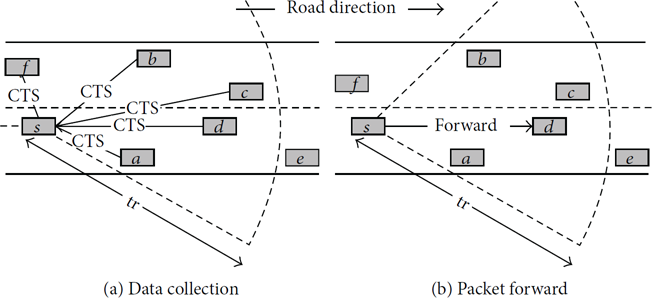
The RTS/CST scheme and forward strategy.

The data collection result can be treated as a snapshot of floating car data. After all vehicles on the road segment are collected or one of the disconnection states occurs, the current traffic speed will be estimated. Specifically, speed estimation algorithm is invoked if one of the following conditions is satisfied: (1)

Packet reaches a new road segment or destination.

(2)

Sparse connection or partial connection occurs.

(3)

The specified time interval has elapsed.

Condition (2) has been shown in lines (7) and (9) of Algorithm 1. Condition (3) is used to handle the special case that the traffic density is low but current vehicle moves slowly (e.g., stop for red light or temporary parking).

After the speed has been estimated, the solution also uses greedy forwarding algorithms to send the estimated speed back to the source vehicle. When the source vehicle receives the estimated speed, it will store the data locally for further usage. It is possible to receive multiple feedbacks for a single road segment. In this case, the one with the latest time stamp will be kept.

4.2. Traffic Speed Estimation

The traffic speed estimation problem has been formulated in Section 3. If we look at the objective function in (3), it looks like an optimization problem. However, it can not be directly solved by any optimization methods, because we are using sparse data (traffic snapshot) to estimate the dense data (traffic condition). And the dense data is unknown but has correlations with the sparse data. To estimate the speed, we need to model the relationship between the data we have and the data we want to get.

In this research, instead of training a model by ourselves, which requires extensive dataset and computation, we decide to utilize existing macroscopic traffic models developed in traffic engineering. Macroscopic traffic model studies the relationship among density, flow, and speed. In our research, we select Underwood model [15], which is a typical density-speed model.

The reasons we choose Underwood density-speed model are twofold. Firstly, several properties can be obtained from the floating data snapshot, like speed, density, vehicle position, and so forth. We need to select suitable features to build the model. Many existing works selected speed [8, 14, 17]. However, we observe that the variance of speed within a period of time is significant. To determine the variance of the speed, we analyze the traffic trace data from Cologne (details are introduced in Section 6), and the VMR (variance-to-mean ratio) of speed is 8.7, while the VMR of density is 4.5. Figure 5 shows the distribution of speed and density. Therefore, density is more stable than speed and can better reflect the traffic condition in a time period. Secondly, many macroscopic density-speed models have been calibrated using site data, for example, Greenberg, Underwood, and Drake [31]. Different models have different strength and weakness. Underwood is more accurate for uncongested condition compared with other models. Judging from Figure 5(b), the probability of uncongested condition is much higher than congested condition.

The original Underwood model can be described as

\begin{matrix} v_{e s t} = v_{f} e^{- k / k_{c}}, \end{matrix}

(4)

where

v_{f}

is the free flow speed and

k_{c}

is the optimum density. That is the density corresponding to the maximum traffic flow and k is current density. Figure 4 shows a typical curve of Underwood model.

Figure 4

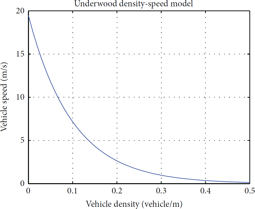
Underwood density-speed traffic model with $v_{f} = 20$ , $k_{c} = 0.1$ .

Figure 5

The distribution of different vehicle properties.

When optimum traffic density $k_{c}$ occurs, the average vehicle speed is $v_{f} / 2$ [15]. We further assume adjacent vehicles keep a safety distance, which means if a vehicle applies maximum deceleration and stopped, a following vehicle must be able to stop before hitting the previous one. We adopt the safety distance defined in [32] as

\begin{matrix} D_{s a f e} = c_{a} \ddot{x} + c_{v} \dot{x} + c_{p}, \end{matrix}

(5)

where

\ddot{x}

and

\dot{x}

denote the acceleration and velocity of vehicles, respectively. For simplicity,

c_{a}

is set to be

0

c_{v}

is set to be

2

seconds (two-second rule [33]), and

c_{p} = 10

m. In this case, the optimum density

k_{c}

can be represented as

\begin{matrix} k_{c} = \frac{1}{D_{s a f e} (c_{v} = v_{f} / 2)} = \frac{1}{(v_{f} / 2) \times 2 + 10} = \frac{1}{v_{f} + 10} . \end{matrix}

(6)

Another issue is how to determine current density from the collected floating car data snapshot. As described in (2), λ is an unknown value. Now, we want to estimate λ from the collected floating car data snapshot.

From the floating car data snapshot we collected, we can construct the vector of distances between adjacent vehicles as $V_{r}^{d} = (X_{1}, X_{2}, \dots, X_{n - 1})$ , where $X_{i} = ‖v_{i} \cdot p o s, v_{(i + 1)} \cdot p o s‖$ . Applying maximum likelihood parameter estimation formula for exponential distribution, λ can be estimated as

\begin{matrix} λ = \frac{1}{\bar{X}} . \end{matrix}

(7)

Considering the traffic regulations, we assume free flow speed is the same as maximum allowed speed; that is, $v_{f} = v_{m}$ . Combining (4), (6), and (7) together, we get

\begin{matrix} v_{e s t} = v_{m} e^{- (v_{m} + 10) / \bar{X}}, \end{matrix}

(8)

where

\bar{X}

is the average vehicle distance per lane and

\begin{matrix} \bar{X} = \frac{\sum_{i = 0}^{i < n - 1} X_{i}}{(n - 1)} \times r \cdot l . \end{matrix}

(9)

It is also possible to fail to collect traffic information for a road segment. This is mainly caused by the sparse traffic. In this case, we assume the average vehicle distance is larger than $t r$ and $\bar{X} = t r$ .

The speed for a specific road segment can be estimated using (8) and (9). The only variables in these equations are the distances among vehicles, which can be obtained from traffic information collection results.

5. MICE in Route Planning Application

The previous section introduced how to collect traffic data and how to estimate traffic speed for a single road segment in MICE. In this section, we apply the proposed solution to a typical and popular ITS application: real-time route planning. This application utilizes the estimated traffic speed to find a shortest-time route for a vehicle. To find the shortest-time route, traffic condition of multiple road segments needs to be collected and estimated.

However, designing such an application is not trivial. To find a global shortest-time path, traffic information of all roads is prerequisite. But considering a city with thousands of roads in real world, it is not feasible to collect information of all roads since the search space is extremely huge. To make the solution practical, we have to be tolerant with a suboptimal solution by collecting traffic information for part of the roads and then make decision.

Since the traffic information is unknown and should be estimated in real-time, the shortest-time route planning problem is a typical stochastic shortest path problem with recourse (SSPPR) in graph theory, which explores adjacent nodes in a graph until finding the destination. Before exploring a node, the weight of the associated edges is unknown. The problem has been proved to be NP-complete [34] and hence has no polynomial time solution unless P = NP.

Our objective here is not to propose a better approximation algorithm for this difficult problem. Instead, we just want to demonstrate the application of our proposed estimation solution in a specific scenario. To solve this problem, we designed a heuristic solution according to two common senses: (1) the longer the path is, the longer the time it may take. (2) It makes no sense to choose another longer path when shortest path is not congested. We name the candidate path selection algorithm Backoff-and-Fork or BnF in short. The basic idea is derived from the two common senses. For (1), we define a total length constraint, which means the total length of a candidate path can not exceed the threshold. For (2), we define a speed threshold, which means if the estimated speed of the shortest path road is slower than the threshold, other nearby alternative paths will be searched.

The complete BnF algorithm is shown in Algorithm 2. At the beginning, the algorithm will only choose the road segments on the shortest path as candidate paths (lines (1)–(3)). Then the data collection request packets are sent to all candidate paths. After that, whenever a packet arrives at a new road segment, it will collect traffic information of all neighbor road segments that have not been collected and then estimate speed (lines (7)–(9)). If the estimated speed is good enough, it will go on with the next road segments. However, if the speed is lower than the predefined threshold (line (10)), the algorithm will send a backoff packet to the previous road segment (backoff). Then, all the neighbor road segments that have not been selected as candidate path will be used as a starting point to build a new shortest path to end point (fork), and the newly built shortest path will be added to the candidate path set if the length has not exceeded the threshold (lines (11)–(13)). To avoid overlapping between the new and old shortest path, the paths connecting existing candidate paths are excluded when executing the shortest path algorithm (line (12)).

Algorithm 2: Backoff-and-Fork candidate path selection.

Input: RN: The road network.

Input: Navigation starting point $n_{s}$ , end point $n_{e}$ and current road intersection $n_{c}$ .

Input: fThreshold: The speed threshold.

Input: Θ: The length threshold.

// Initialize.

(1) for all sp ∈ ShortestPath(RN, $n_{s}$ , $n_{e}$ ) do

(2) $s p$ . IsCandidate = True

(3) end for

// On packet arrive at road segments.

(4) if $n_{c} = = n_{e}$ then

(5) return

(6) end if

(7) for all $r s \in n_{c}$ . NeighborRoad do

(8) if rs. IsCandidate and not rs. IsCollected then

// Collect data on road rs.

(9) EstimatedSpeed = SpeedEstimate(rs)

(10) if EstimatedSpeed/ $(r s \cdot v_{m}) < f$ Threshold then

// Backoff and fork.

(11) for all $r p \in n_{c}$ . NonCandidateNeighborRoad do

(12) $Length$ = ShortestPathLength( $RN - r p$ , $r p \cdot e$ , $n_{e}$ )

(13) if Length + CollectedLengh < Θ then

(14) for all r ∈ ShortestPath( $RN - r p$ , $r p \cdot e$ , $n_{e}$ ) do

(15) r. IsCandidate = True

(16) end for

(17) end if

(18) end for

(19) end if

(20) end if

(21) end for

Figure 6 can be used to demonstrate how the BnF algorithm works. The starting point and end point are S and E, respectively. In the initial phase, the shortest path $(S, c, h, E)$ is selected. Then, $〈S c〉$ is collected. The estimated speed of $〈S c〉$ is good, so it continues with the next candidate path $〈c h〉$ . At this time, the estimated speed of $〈c h〉$ is too slow, and the algorithm will back off to c and fork to the neighbors d and f. The new shortest paths to E are found to be $(d, g, e)$ and $(f, h, e)$ . Then, new candidate paths $〈c d〉$ , $〈d g〉$ , $〈g E〉$ , $〈c f〉$ , and $〈f h〉$ are added to the search list.

Figure 6

An example of Backoff-and-Fork algorithm.

The algorithm will terminate when the request packets arrive at the navigation destination.

6. Performance Evaluation

6.1. Experiment Setup

In this section, we evaluate the performance of MICE using both small-scaled testbed implementation and traffic trace based large-scaled simulation. We choose two evaluation methods because both of them have advantages and disadvantages. The traffic trace provides a realistic evaluation scenario. However, some parameters like the average vehicle density or speed are not configurable. Consequently, we can not use the trace to test the impact of these parameters. On the contrary, the testbed is more flexible, but the road topology and traffic scale are very limited. Figures 7 and 8 show the testbed, road network topology, and flow chart of the evaluation.

Figure 7

iTranSNet testbed and cologne topology.

Figure 8

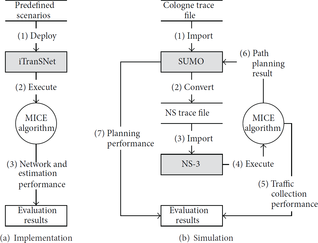
Evaluation flow chart.

We implemented the MICE on iTranSNet [35]. The iTranSNet is a testbed with several programmable mini cars, which is modified from toy cars by ourselves. The moving speed of the toy cars is very slow, approximately 0.4 m/s, and we can control the speed with program. The size of iTranSNet platform is 3 m × 6 m. The road network topology of iTranSNet is illustrated in Figure 7(a). The mini cars are controlled by onboard MICAz wireless sensor nodes. The MICAz sensor nodes can also communicate with each other using IEEE 802.15.4. The MICE algorithm is implemented on MICAz with TinyOS [36]. In our implementation, we set the transmission power to the lowest level (approximately 1 m) to enable multihop among vehicles. The positions of all mini cars can be determined by sensors on iTranSNet. The vehicles follow the traffic light control rules [37]. We run the experiments under several configurations: dense traffic (25 cars), sparse traffic (12 cars), and some intermediate values. The experiments are repeated 50 times with arbitrary route planning starting and end points.

For simulation, we use the traffic trace dataset from Cologne in Germany provided by [38], where detailed analysis of the trace can also be found. Traffic simulator SUMO [39] is used to simulate the traffic mobility and network simulator NS-3 [40] is used to simulate VANETs communication and run MICE algorithm. Table 1 shows other parameter settings for NS-3. The simulation process works as depicted by Figure 8(b): firstly, a subset of the traffic trace file (geographical region $[50.9222$ –50.9552, 6.9077–6.9624]) is imported into SUMO to generate the trace file that can be used by NS-3. After that, NS-3 simulator will run the MICE algorithm using the mobility trace and get the route planning result as output. Meanwhile, the network performance data are generated. Finally, the route planning results are imported into SUMO again to evaluate the route planning performance. A Python script is used to automate this process and the simulation is repeated 50 times with arbitrary starting and end points as well as starting time.

Table 1

NS-3 simulation parameters.

Parameter	Value
MAC/PHY standard	IEEE 802.11p SCH
Propagation delay mode	Constant speed
MAC type	Ad hoc Wi-Fi MAC
Propagation loss model	Range propagation loss model
Transmission range	100 m
Packets carry duration	1 second
Neighbor wait duration	0.3 second

6.2. Traffic Collection Evaluation

To evaluate the performance of traffic collection protocol, we are interested in the network latency and the network overhead. The network latency is defined as $T_{l a t e n c y} = T_{r e q} - T_{l a s t_f e e d b a c k}$ , where $T_{r e q}$ is the time stamp of the collection request which is sent and $T_{l a s t_f e e d b a c k}$ is the time stamp of the last feedback which is received. We use the time stamp of the last packet instead of the first one because Algorithm 1 may send multiple feedbacks; the last one is the one we finally use and it usually contains more accurate estimation than the previous ones. The network overhead is represented by the total number of packets that have been sent.

Figure 9 shows the traffic collection evaluation results. Two major factors are evaluated: path length and traffic density. The results (distance and time cost) of multiple evaluations are added together and plotted in Figure 9. From Figure 9(a), we can see that the latency increases as the path length. And for the same length, the latency for sparse traffic is usually larger than the case of dense traffic. This is caused by the frequent packet carrying in sparse traffic condition. Figure 9(b) shows that the total number of packets transmitted also increases as the path length. For the same length, more packets are transmitted in dense traffic condition. This is because of the RTS/CST scheme depicted in Figure 3. When the traffic is dense, after an RTS is sent, more CTS replies are generated and transmitted over the air.

Figure 9

Network evaluation results using iTranSNet testbed.

Figure 10 illustrates the traffic collection evaluation results using traffic trace. We run the experiments many times and sum up the distance and time consumption. As we can see, the increase trend of latency and the number of packets sent are similar as the results obtained by testbed. Moreover, the results are more convincing since the road condition, vehicle speed, and distribution are more realistic. The network latency of is less than 1 min/km. In real application scenario, the delay is acceptable.

Figure 10

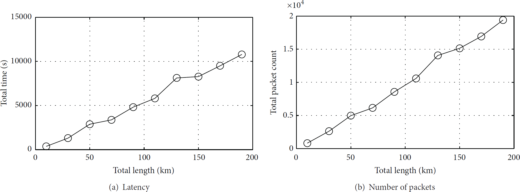
Network evaluation results using traffic trace.

6.3. Speed Estimation Evaluation

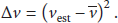
To evaluate the performance of traffic speed estimation algorithm, we consider the impact of traffic density and time window length p in traffic condition (Definition 4). Data of a single road segment is collected and estimated. The road segment is selected randomly and the experiments are repeated 50 times. We compare our solution with VAN [8], which calculate the mean speed of collected vehicles to represent the traffic speed. The mean estimation error is calculated using (10). Therefore, the smaller the error is, the better the method works

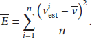
\begin{matrix} \bar{E} = \sum_{i = 1}^{n} \frac{{(v_{e s t}^{i} - \bar{v})}^{2}}{n} . \end{matrix}

(10)

Figure 11 illustrates the relationship between traffic density and the estimation error. The unit of density is the number of vehicles per meter per lane. From this figure, we can see that, in most of the cases, the estimation errors of MICE are smaller than VAN, which indicates that our method outperforms VAN in traffic speed estimation. The key insight is that, compared with mean speed used by VAN, the density-speed model used by MICE can better reveal the truth in most cases. However, the estimation error of MICE has a remarkable increase trend when the traffic density is high. There are two reasons for this. First, Underwood density-speed model we select performs better in low density scenario. Second, when vehicle density reaches 0.2 (headway distance is 5 m), the traffic is highly congested and the vehicles are almost stopped. Then, the variance is not significant, the mean speed method used by VAN can even better reflect the ground truth.

Figure 11

Traffic density and speed estimation accuracy.

Figure 12 shows the relationship between estimation error and time window size. The size of the time window affects the value of traffic condition mean speed $\bar{v}$ . If the time window is small enough, $\bar{v}$ is close to instant speed. In this case, the estimation errors tend to be significant. This trend can be observed in Figure 12(a). For Figure 12(a), the vehicle density is fixed at 0.05 vehicle per meter per lane. For Figure 12(b), the density of traffic trace can not be controlled. In most of the cases, MICE performs better than VAN, which further validates that density-speed model is a better option than mean speed. Another observation is that the relationship between time window size and the accuracy of the algorithm is not obvious. This result reveals the insight that, in real case, the traffic condition is stable within certain time period (e.g., within 200 seconds). It is also noticeable that the errors in Figure 12(b) are much larger than Figure 12(a). This is mainly because, in real traffic traces, the variation of car speed is much larger (0–80 km/h) than that in testbed (0–1.5 km/h).

Figure 12

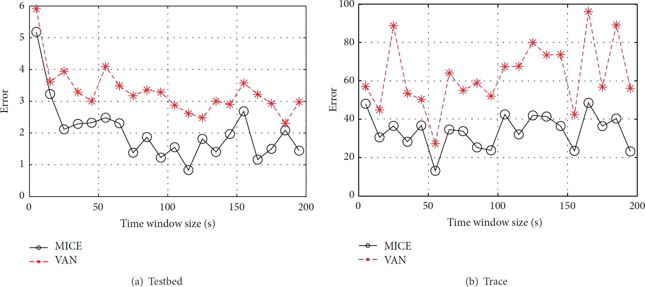
Time window size and speed estimation accuracy.

6.4. Route Planning Application

Finally, we evaluate the performance of different speed estimation solutions by putting them into route planning application. We calculate the shortest-time path using the estimated traffic speed from these solutions and then let the vehicles travel along the shortest-time path in SUMO or iTransNet testbed to obtain the actual time consumption. In this way, we can find out the performance of these solutions in real applications.

We firstly evaluate the successful collection ratio of road segments. The collection ratio is defined as $c o u n t (C_{i}) / c o u n t (C)$ , where $c o u n t (C)$ is the number of road segments in all candidate paths and $c o u n t (C_{i})$ is the number of road segments that has been collected successfully. The collection failure is usually caused by packets loss or extreme sparse traffic. In Figure 13, a steady increase for successful collection ratio can be found, from about 75% to 95%. However, the increase trend is not obvious after the density reaches a specific threshold. The reason for this is that, after the threshold is reached, the VANETs approximately become a fully connected graph. Therefore, the packet loss rate is then reduced dramatically. The average collection ratio using trace on NS-3 is above 90% since the trace is collected during morning rush hour.

Figure 13

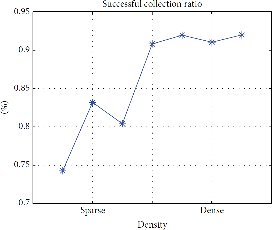
Collection ratio.

The performance of BnF algorithm is also evaluated. The evaluation is only performed with trace data since the results are not obvious on iTranSNet due to the small scale. We compare our heuristic solution with a spatial constrained broadcast solution, which collects traffic information of all roads within an ellipse with navigation starting point and end point as two foci of the ellipse. 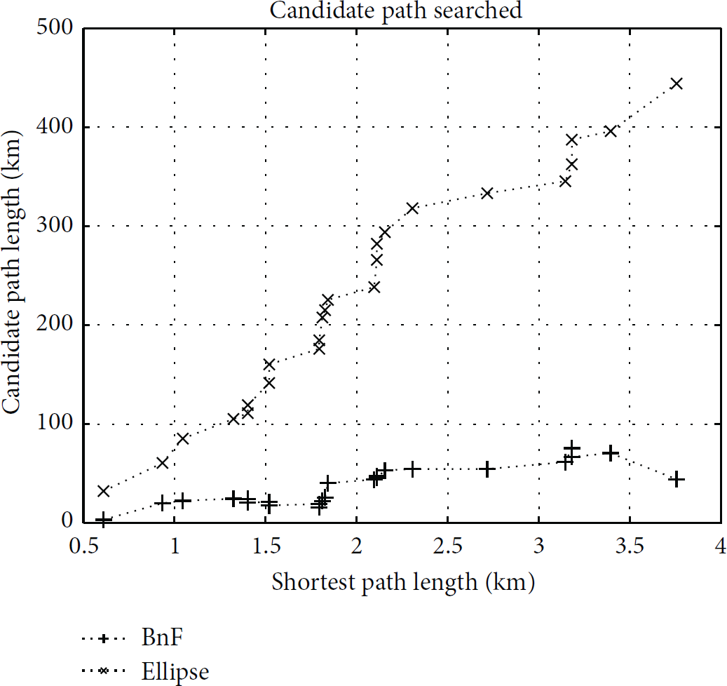In the evaluation, we set the length threshold Θ to 3 times of the shortest path length and then increase the speed threshold $f T h r e s h o l d$ gradually until our solution and the ellipse-based solution have the same or better result when route planning. Then, the total length of the candidate path is depicted in Figure 14. We can see that our BnF algorithm can save up to 75% of the search paths. As a result, the network communication overhead can be reduced significantly.

Figure 14

Candidate path.

Finally, we evaluate the route planning performance using different route planning algorithms. For route planning evaluation, we are interested in the effectiveness of route planning, that is, how much time can be saved, and the travel overhead, that is, how many extra distances have to be travelled in order to bypass the congested road segments. In the evaluation, we compare MICE with two static route planning algorithms: shortest path Dijkstra algorithm (SP, the weight of edges is $‖r‖$ ) and shortest-time Dijkstra algorithm (ST, the weight of edges is $‖r‖ / r \cdot v_{m}$ ) and one dynamic route planning algorithm VAN [8], which uses mean speed to estimate traffic. On iTranSNet, due to hardware limitation, the maximum allowed speed for all road segments is the same; thus the shortest path and the shortest-time planning algorithm are identical. Therefore, we ignore the results for shortest-time planning algorithm on iTranSNet.

Given the same navigation starting and ending points, different route planning algorithms may generate either the same or different route planning results. Figure 15 shows the similarity and differences of the algorithm output. On iTanSNet testbed, the route planning results for SP, VAN, and MICE solutions are quite similar: about 60% of the total tries have the same result, and only 5% of total tries have completely different results. This is caused by the small scale. For traffic trace based simulation, only 30% of the results are identical. It can also be observed that the similarity between MICE and VAN is higher than the two static ones.

Figure 15

Overview of shortest-time path planning results.

The overall efficiency charts in Figures 16 and 17 reveal that our algorithm works better in dense traffic conditions, compared with spare ones. This conclusion does not contradict the results from Figure 11, because the shortest-time route planning algorithms can bypass dense road segments and select sparse ones automatically. In sparse traffic scenarios, the performance of the three algorithms is quite similar due to traffic congestion, although MICE indeed has some improvement. In contrast, MICE has about 25% time saving compared with Dijkstra algorithm and about 15% time saving compared with VAN. For the trace based simulation case in Figure 18, MICE has about 15% time saving compared with Dijkstra algorithm and about 5% time saving compared with VAN.

Figure 16

Performance results for path planning application in dense traffic using iTranSNet testbed.

Figure 17

Performance results for path planning application in sparse traffic using iTranSNet testbed.

Figure 18

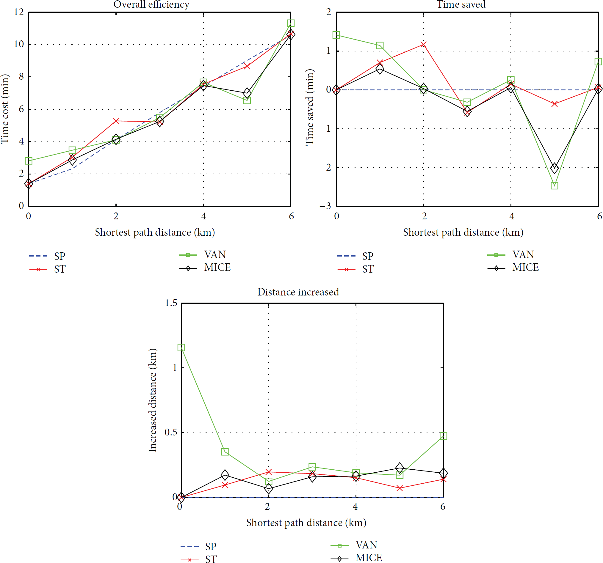
Performance results for path planning application using traffic trace.

The time saved charts in Figures 16 and 17 use the same evaluation results as overall efficiency but use the time cost for the shortest path as baseline for better understanding. An interesting observation can be found in which, in the trace based simulation, sometimes the shortest-time algorithm spends even longer time than shortest path one. The result is consistent with our experiences. However, analyzing the result is out of the scope of this paper.

Finally, the distance increased chart shows the travel overhead to bypass the congested road. It also uses shortest path length as baseline. It is observed that the travel overhead is controlled within 10%. For the trace based simulation in Figure 18, it is interesting to discover that the overhead of MICE is only a little higher than the shortest-time algorithm and about 10% lower than VAN. In these figures, the improvement of MICE is not that obvious. As depicted in Figure 15, about 75% of the path planning results for VAN and MICE are the same. In order to reflect the real performance, we did not remove these duplicated results in the charts.

7. Conclusion

In this paper, we have proposed MICE, a traffic estimation solution by collecting and analyzing surrounding traffic information using VANETs in real-time. The traffic collection solution is infrastructure-free and scalable compared with conventional infrastructure based ones. We have also employed a novel density-speed traffic model to estimate traffic condition using the collected floating car data. Then, we have applied the proposed algorithm to a shortest-time route planning applications to demonstrate the performance of the solution. Extensive evaluations using both testbed based implementation and trace based simulation have been conducted. The results have shown that our solution can outperform some existing ones in terms of network transmission overhead, route planning effectiveness, and traffic overhead.

Footnotes

Summary of Notations

Conflict of Interests

The authors declare that there is no conflict of interests regarding the publication of this paper.

Acknowledgment

This research is partially supported by Microsoft Research Asia Accelerating Urban Informatics with Azure Program.

References

Cao

MICE: A real-time traffic estimation based vehicular path planning solution using VANETs

Proceedings of the 1st International Conference on Connected Vehicles and Expo (ICCVE ′12)

December 2012

172 178

10.1109/iccve.2012.39

2-s2.0-84879491200

Shimamoto

An open traffic light control model for reducing vehicles' CO₂ emissions based on ETC vehicles

IEEE Transactions on Vehicular Technology 2012 61 1 97 110

10.1109/tvt.2011.2168836

2-s2.0-84862909111

Tian

Yao

Wang

Video processing techniques for traffic flow monitoring: a survey

Proceedings of the 14th IEEE International Intelligent Transportation Systems Conference (ITSC ′11)

October 2011

1103 1108

10.1109/itsc.2011.6083125

2-s2.0-83755178658

Singh

Estimation of traffic densities for multilane roadways using a markov model approach

IEEE Transactions on Industrial Electronics 2012 59 11 4369 4376

10.1109/tie.2011.2180271

2-s2.0-84862993755

Kong

Q.-J.

Chen

Liu

An approach to Urban traffic state estimation by fusing multisource information

IEEE Transactions on Intelligent Transportation Systems 2009 10 3 499 511

10.1109/TITS.2009.2026308

2-s2.0-70349178654

Jeong

Guo

D. H. C.

Trajectory-based data forwarding for light-traffic vehicular Ad Hoc networks

IEEE Transactions on Parallel and Distributed Systems 2011 22 5 743 757

10.1109/tpds.2010.103

2-s2.0-79953310708

Stanica

Fiore

Malandrino

Offloading floating car data

Proceedings of the IEEE 14th International Symposium on a World of Wireless, Mobile and Multimedia Networks (WoWMoM ′13)

June 2013

1 9

10.1109/wowmom.2013.6583391

2-s2.0-84883697774

Chen

Zhu

VAN: vehicle-assisted shortest-time path navigation

Proceedings of the 7th IEEE International Conference on Mobile Adhoc and Sensor Systems (MASS ′10)

November 2010

442 451

10.1109/mass.2010.5663936

2-s2.0-78650979795

Collins

Muntean

G.-M.

A vehicle route management solution enabled by wireless vehicular networks

Proceedings of the IEEE INFOCOM Workshops

April 2008

IEEE

1 6

10.1109/infocom.2008.4544658

2-s2.0-51049090418

10.

Calabrese

Colonna

Lovisolo

Parata

Ratti

Real-time urban monitoring using cell phones: a case study in Rome

IEEE Transactions on Intelligent Transportation Systems 2011 12 1 141 151

10.1109/tits.2010.2074196

2-s2.0-79952071926

11.

Nadeem

Dashtinezhad

Liao

Iftode

Trafficview: traffic data dissemination using car-to-car communication

ACM SIGMOBILE Mobile Computing and Communications Review 2004 8 3 6 19

12.

Lochert

Scheuermann

Wewetzer

Luebke

Mauve

Data aggregation and roadside unit placement for a vanet traffic information system

Proceedings of the 5th ACM International Workshop on VehiculAr Inter-NETworking (VANET ′08)

September 2008

ACM

58 65

10.1145/1410043.1410054

2-s2.0-59249090296

13.

Rybicki

Scheuermann

Koegel

Mauve

PeerTIS—a peer-to-peer traffic information system

Proceedings of the 6th ACM International Workshop on VehiculAr Inter-NETworking (VANET ′09)

September 2009

23 32

10.1145/1614269.1614275

2-s2.0-70350680651

14.

Shu

Huang

H.-Y.

Luo

P.-E.

M.-Y.

Performance evaluation of vehicle-based mobile sensor networks for traffic monitoring

IEEE Transactions on Vehicular Technology 2009 58 4 1647 1653

10.1109/tvt.2008.2005775

2-s2.0-66149152721

15.

May

Traffic Flow Fundamentals 1990

Prentice Hall

16.

Arbabi

M. H.

Weigle

M. C.

Using vehicular networks to collect common traffic data

Proceedings of the 6th ACM International Workshop on VehiculAr Inter-NETworking (VANET ′09)

September 2009

New York, NY, USA

ACM

117 118

10.1145/1614269.1614289

2-s2.0-70350647144

17.

Liu

Flow-based travel plan via VANET

International Journal of Digital Content Technology and its Applications 2011 5 6 163 171

10.4156/jdcta.vol5.issue6.19

2-s2.0-79960030326

18.

Sen

Maurya

Raman

Mehta

Kalyanaraman

Vankadhara

Roy

Sharma

Kyun queue: a sensor network system to monitor road traffic queues

Proceedings of the 10th ACM Conference on Embedded Network Sensor Systems (SenSys ′12)

November 2012

Toronto, Canada

ACM

127 140

10.1145/2426656.2426670

19.

Dornbush

Joshi

Streetsmart traffic: discovering and disseminating automobile congestion using vanet

Proceedings of the Vehicular Technology Conference (VTC-Spring ′07)

April 2007

11 15

20.

Naumov

Baumann

Gross

An evaluation of inter-vehicle ad hoc networks based on realistic vehicular traces

Proceedings of the 7th ACM International Symposium on Mobile Ad Hoc Networking and Computing (MobiHoc ′06)

May 2006

108 119

2-s2.0-33748041133

21.

Garelli

Casetti

Chiasserini

Fiore

Mobsampling: V2v communications for traffic density estimation

Proceedings of the 73rd IEEE Vehicular Technology Conference (VTC-Spring ′11)

2011

1 5

22.

Lakas

Shaqfa

Geocache: sharing and exchanging road traffic information using peer-to-peer vehicular communication

Proceedings of the IEEE 73rd Vehicular Technology Conference (VTC Spring ′11)

May 2011

IEEE

1 7

10.1109/vetecs.2011.5956785

2-s2.0-80052011681

23.

Ding

J.-W.

Wang

C.-F.

Meng

F.-H.

T.-Y.

Real-time vehicle route guidance using vehicle-to-vehicle communication

IET Communications 2010 4 7 870 883

10.1049/iet-com.2009.0163

MR2778371

2-s2.0-77956914023

24.

Wedde

H. F.

Senge

Beejama: a distributed, self-adaptive vehicle routing guidance approach

IEEE Transactions on Intelligent Transportation Systems 2013 14 4 1882 1895

10.1109/tits.2013.2269713

2-s2.0-84890436389

25.

Hodge

Krishnan

Jackson

Austin

Polak

Short-term traffic prediction using a binary neural network

Proceedings of the 43rd Annual Universities' Transport Studies Group Conference (UTSG ′11)

2011

Milton Keynes, UK

Open University

26.

Kanoh

Hara

Hybrid genetic algorithm for dynamic multi-objective route planning with predicted traffic in a real-world road network

Proceedings of the 10th Annual Genetic and Evolutionary Computation Conference (GECCO ′08)

July 2008

New York, NY, USA

ACM

657 664

2-s2.0-57349112331

27.

Comert

Cetin

Analytical evaluation of the error in queue length estimation at traffic signals from probe vehicle data

IEEE Transactions on Intelligent Transportation Systems 2011 12 2 563 573

10.1109/TITS.2011.2113375

2-s2.0-79958105728

28.

Mung

G. K. S.

Poon

A. C. K.

Lam

W. H. K.

Distributions of queue lengths at fixed time traffic signals

Transportation Research Part B: Methodological 1996 30 6 421 439

10.1016/0191-2615(96)00009-4

2-s2.0-0030382880

29.

Bai

Krishnamachari

Spatio-temporal variations of vehicle traffic in VANETs: facts and implications

Proceedings of the MobiHoc6th ACM International Workshop on VehiculAr Inter-NETworking (VANET ′09)

September 2009

ACM

43 52

10.1145/1614269.1614278

2-s2.0-70350662582

30.

Karp

Kung

H. T.

Gpsr: greedy perimeter stateless routing for wireless networks

Proceedings of the 6th Annual International Conference on Mobile Computing and Networking (MobiCom ′00) 2000

New York, NY, USA

ACM

243 254

31.

Ardekani

Ghandehari

Nepal

Macroscopic speed-flow models for characterization of freeway and managed lanes

Institutul Politehnic din Iasi. Buletinul. Sectia Constructii. Arhitectura 2011 57 1

32.

Godbole

D. N.

Lygeros

Longitudinal control of the lead car of a platoon

IEEE Transactions on Vehicular Technology 1994 43 4 1125 1135

10.1109/25.330177

2-s2.0-0028539253

33.

Wikipedia

Two-second rule—wikipedia, the free encyclopedia@online

2013, https://en.wikipedia.org/wiki/Two-second_rule

34.

Andreatta

Romeo

Stochastic shortest paths with recourse

Networks 1988 18 3 193 204

10.1002/net.3230180306

MR953922

35.

Poly

iTransnet

2010, http://imc.comp.polyu.edu.hk/isensnet/doku.php?id=research

36.

Levis

Madden

Polastre

Szewczyk

Whitehouse

Woo

Gay

Hill

Welsh

Brewer

Culler

Weber

Rabaey

Aarts

Tinyos: an operating system for sensor networks

Ambient Intelligence 2005

Berlin, Germany

Springer

115 148

37.

Zhou

Cao

Zeng

Adaptive traffic light control in wireless sensor network-based intelligent transportation system

Proceedings of the 72nd IEEE Vehicular Technology Conference Fall (VTC ′10)

September 2010

Ottawa, Canada

IEEE

1 5

10.1109/VETECF.2010.5594435

38.

Uppoor

Fiore

Large-scale urban vehicular mobility for networking research

Proceedings of the IEEE Vehicular Networking Conference (VNC ′11)

November 2011

62 69

10.1109/vnc.2011.6117125

2-s2.0-84857559625

39.

Behrisch

Bieker

Erdmann

Krajzewicz

Sumo—simulation of urban mobility: an overview

Proceedings of the 3rd International Conference on Advances in System Simulation (SIMUL ′11)

October 2011

Barcelona, Spain

40.

Henderson

Lacage

Riley

Dowell

Kopena

Network simulations with the ns-3 simulator

Proceedings of the ACM SIGCOMM Conference on Data Communication (SIGCOMM ′08)

2008

Seattle, Wash, USA

Accurate Real-Time Traffic Speed Estimation Using Infrastructure-Free Vehicular Networks

Abstract

1. Introduction

2. Related Work

2.1. Traffic Information Collection

2.2. Traffic Speed Estimation

3. Problem Statement

3.1. Preliminaries

Definition 1 (road segment).

Definition 2 (vehicular network).

Definition 3 (floating car data snapshot).

Definition 4 (traffic condition).

Definition 5 (traffic density).

3.2. Problem Formulation

4. Solution

4.1. Traffic Information Collection

Algorithm 1: Packet forwarding algorithm on receiving a new packet.

4.2. Traffic Speed Estimation

5. MICE in Route Planning Application

Algorithm 2: Backoff-and-Fork candidate path selection.

6. Performance Evaluation

6.1. Experiment Setup

6.2. Traffic Collection Evaluation

6.3. Speed Estimation Evaluation

6.4. Route Planning Application

7. Conclusion

Footnotes

Summary of Notations

Conflict of Interests

Acknowledgment

References