Design and Implementation of Spatial Operators and Energy-Efficient Query Processing Strategy in Wireless Sensor Network Database System

Abstract

Database applications in wireless sensor networks very often demand data collection from sensor nodes of specific target regions. Design and development of spatial query expressions and energy-efficient query processing strategy are important issues for sensor network database systems. The existing sensor network database systems lack the needed sophistication for the space calculation of the target sensor nodes; hence, unnecessary query/data transmissions are required between the sensor nodes and the server. This paper describes our spatial operations and energy-efficient query processing methods that are designed and implemented in our sensor network database system called ${\text{SNQL}}^{+s}$ . With a set of spatial operators based on geometric parameters, such as Envelope, NearBy, Distance, Direction, and set theoretic operators, ${\text{SNQL}}^{+s}$ allows sensor network applications to easily specify the target space of interest. Our energy-efficient query processing strategy implements an in-network query management based on the lowest common ancestor (LCA) algorithm, so that the query processing cost for calculating the target spaces is greatly reduced by avoiding the need of heavy query/data transmissions between the base-station and target nodes. Performance evaluation shows that our proposed design and implementation of spatial query expressions and processing strategy achieve improved energy efficiency for database operations in the wireless sensor network.

1. Introduction

Sensor networks are increasingly used in a wide range of modern applications, including disaster management, precision agriculture, healthcare, traffic management, and ecological monitoring as one of the most useful emerging information management systems [1–5]. In many earlier developments of sensor networks, sensor nodes were viewed as network components; therefore, they were designed mainly to propagate stream data over a network to the base-station using preinstalled data aggregation instructions from the network perspectives [6, 7]. From the data management perspectives, on the other hand, a sensor network is viewed as a real-world resource of time-variant data in a sense similar to a huge database reservoir. By grafting the traditional database management perspectives to the sensor network, sensor networks have become more functional in data processing so as to be able to serve a wider range of modern sensor network applications.

The typical procedure of query processing in a sensor network database system can be summarized as follows: (1) an application issues a query over to the sensor network; (2) the designated sensor nodes execute the query; and (3) data are aggregated along the topological alignment of networked sensor nodes back to the base-station, where the application processes them on the fly or stores them in a back-end database. A few works on sensor network database systems have been reported [8–12].

The sensor nodes in a wireless sensor network have battery limitation and consume more energy for query/data transmission over the networked nodes than for data reading at the nodes. Therefore, how to reduce (and balance) the energy consumption for query/data transmission is an important research issue. Query processing in wireless sensor networks exploits in-network processing methods and routing plans in an effort to minimize and balance the battery consumption during the course of query/data transportation [9, 10, 13].

Applications of database management in the sensor networks typically require data collection from the nodes of some geographical areas of interest as a target space, such as an area damaged by forest fire, an area designated as the peak, an area of a given coordinate, and areas of an abrupt increase in traffic, north of a certain point. Reducing the energy consumption in the wireless sensor network is an important issue to achieve efficient data reading operations at individual sensor nodes and maintain energy balance for the entire sensor network as well. The design and development of spatial query operations and associated query processing strategies are important issues in sensor network databases for achieving energy-efficient data management.

Spatial queries in sensor network databases often have multiple targeting structures, such as “read temperatures from the regions where the humidity is lower than 10% in the west slope of the mountain.” This query indicates the first target space as “the west slope of the mountain” and the next target space is formed according to the humidity readings from the sensor nodes in the first target area. It seems that this query is intended to monitor and predict a possible forest fire.

A few sensor network database systems have been designed [8–12]. However, for their limited spatial expressions, they require multiple query disseminations and data collections by issuing a query to select sensor nodes of the first target region (i.e., the west slope in the above example) and another query to collect data from sensor nodes of the second target region(s) with humidity lower than 10% in the example. In our proposed approach, on the other hand, a single query with spatial operations manages multiple targeting by using an in-network query processing method so that the identification of subsequent target region(s) is done at some intermediate nodes called lowest common ancestor (LCA) nodes without traversing to and from the base-station.

This paper presents our design and implementation of spatial operations and associated query processing algorithm in an effort to better support sophisticated demands of sensor network applications. We have designed spatial operators based on geometric parameters, such as Envelope, Nearby, Distance, and Direction, as well as binary spatial operators, such as Intersection, Union, and Difference in an attempt to extend our previous sensor network database SNQL [8, 14]. We also have developed our query processing method called LCA-based in-network query processing (in short, LCA-algorithm). We have defined a LCA node as one of the parent sensor nodes that minimally covers all the leaf nodes of the target region that participate in the query processing. At the LCA node, the new target region will be identified according to the data read from the nodes of the initial target region, and then the registered query at the LCA node is reformed and redisseminated for final reading without traversing to and from the base-station. Our proposed spatial query expressions and LCA algorithm together will efficiently reduce the query processing cost in the wireless sensor network.

The contribution of this paper is summarized as follows.

• (i)

We have extended our previous work on sensor network query language SNQL [8, 14] by incorporating various spatial operators, so that more sophisticated expressions of target space are made possible in our new system called ${\mathrm{S}\mathrm{N}\mathrm{Q}\mathrm{L}}^{+s}$ .

(ii)

We designed an efficient query processing strategy by employing the concept of lowest common ancestor (LCA), which implements an efficient in-network query processing for spatial query operations.

The rest of this paper is organized as follows. Section 2 introduces related works, and Section 3 describes the spatial operators. Section 4 explains the LCA-based in-network query processing algorithm. Section 5 explains the architecture of the ${\mathrm{S}\mathrm{N}\mathrm{Q}\mathrm{L}}^{+s}$ , and Section 6 shows the performance evaluation. Finally, conclusions are given in Section 7.

2. Related Work

Madden et al. have proposed TinyDB which is a distributed query processing system running on the Berkeley mote platform on top of TinyOS operating system [9]. It supports acquisitional query processing (ACQP) that has the features of when, where, and in what order the sensor nodes are sampled and which nodes should be included in processing a particular query. It also manages a semantic routing tree (SRT) to store a single one-dimensional interval, representing the range values beneath each of its children in each node. For example, when a query that has a spatial condition, such as “x-coordinate > 100”, arrives at a node, the node checks whether any child's x-coordinate range value overlaps the spatial condition of the given query. If so, it forwards the query down to the child nodes. Thus, SRT supports the efficient dissemination of queries and collection of query results over spatial conditions. However, since spatial expression is limited to disseminating a query only to target nodes with the coordinates in the query, multiple queries are needed if the intermediate query results are used as the conditions for the following queries as given in the aforementioned example.

Di Felice et al. have extended TinyDB to support the spatial expression of queries by means of the longitude and latitude of the nodes indicating their physical locations [15]. To apply spatial operation, the attributes of TinyDB are extended with longitude and latitude to create the preconditions for the georeferencing of the sensor nodes. The extended TinyDB enables the processing of some spatial operators, such as Distance, Inbox, and Beyondboundary. Among these operators, Inbox determines whether a node exists within a given envelope for identifying nodes in a physical space. For example, if one wants to read temperature from a rectangle $(\mathrm{0,0},\mathrm{500,500})$ , “SELECT temperature FROM sensors WHERE Inbox $[0,0,500,500]$ ” is issued. However, since only a few spatial operators are supported, there are limitations in expressing queries related to location information in a sensor network. For instance, it does not support operators to find nodes in a designated direction and to find the node closest to a given position.

Kim et al. proposed Spatial TinyDB, which supports spatial data types and spatial operators by extending TinyDB by incorporating standard geospatial expressions proposed by the Open Geospatial Consortium (OCG) [16, 17]. The spatial TinyDB supports spatial data types, spatial relation operators, spatial analysis operators, and spatial trajectory operators. Their spatial data types are managed in seven types: Point, LineString, Polygon, PolyhedralSurface, MultiPoint, MultiLineString, and MultiPolygon. Also, eight spatial relation operators are given, such as Equals, Disjoint, Touches, Within, Overlaps, Crosses, Intersection, and Contains. Each relation operator receives two spatial objects and returns True or False as the output. Spatial analysis operators include six operators, such as Distance, Intersection, Difference, Union, Buffer, and Convexhull. Each receives two spatial objects and returns a new spatial object as the output. However, since the spatial data types are limited to expressing a region with the coordinates of area, it is not suitable to select an unfixed target region (e.g., the region where the humidity is lower than 10%), and thus it requires multiple queries if intermediate query results are used as the conditions for the following queries.

Yao et al. proposed the Cougar system, in which sensor data is periodically collected from the physical environment and is represented by time series [10, 11]. They proposed query processing over sensor data which are considered as a virtual relational database, so that a user can issue queries without knowing the physical characteristics of the sensor network. In Cougar, it is assumed that each sensor type has a standard abstract data type (ADT) representation which is used at all nodes. Sensors can be treated as ADT objects in query processing, and the user application manages a SQL-like interface through ADT. Here, the simplified schema of the sensor network database contains one relation R(loc point, floor int, s sensorNode), where loc is a point ADT that stores the coordinates of the sensor, floor is the floor where the sensor is located in the data warehouse, and sensorNode is a sensor ADT that supports the methods detectAlarmTemp(threshold). Here, the threshold is the threshold temperature above which abnormal temperatures are returned. For example, if one wants to generate a notification when two sensors within 5 yards of each other simultaneously measure an abnormal temperature, “SELECT R1.s.detectAlarmTemp(100),  R2.s.detectAlarmTemp(100) FROM R R1, R R2 WHERE $SQRT ($SQR(R1.loc.x − R2.loc.x) + $SQR(R1.loc.y − R2.loc.y)) < 5” is issued. However, the location is stored in the front-end server for querying so that query processing takes place on the centralized database. Therefore, if intermediate query results are used as the conditions for the following queries, it also needs to disseminate multiple queries.

Shen et al. proposed SINA [12] which supports SQL-like query and script using a language called Sensor Query and Tasking Language (SQTL). This system is based on a spreadsheet database where each attribute is referred to as a cell, and it incorporates a hierarchical clustering mechanism. SQTL provides primitives for sensor hardware access (e.g., getTemperature, turnOn), location aware (e.g., isNeighbor, getPosition), and communication (e.g., tell, execute) primitives, as well as event handling. These scripts migrate from node to node depending on their parameters by the sensor execution environment (SEE) located in each sensor node. Then, the SEE examines all SQTL messages and performs the appropriate operation. For example, messages with “ALL_NODES” are rebroadcasted to every sensor node, and those with “NEIGHBORS” are forwarded only to nodes that are one-hop-away neighbours in the sensor network. As in these examples, location is used for primitive operations, such as forwarding messages. Therefore, spatial operation does not work efficiently when multiple targets are used.

Amongst the studies related to spatial query processing in sensor networks, some attempt to utilize spatial indexing for query processing. Soheili et al. suggested Spatial Index (SPIX), which applied R-Tree to sensor network [18]. In that, a sensor node forms Minimum Boundary Area (MBA) that includes the location information of itself and of its descendant sensor nodes along the routing pass and manages these in the form of R-tree. The MBA is used to determine whether the spatial query, once received from a higher-level node for sensor data collection within a given area, should be passed to the lower-level nodes. Li et al. proposed back forwarding method, which uses SPIX mechanism for disseminating query and rearranging mechanism for return route of the query result to base-station [19]. By restructuring return path dynamically for the query result, they reduced the energy cost of aggregating the query result. Park et al. suggested Sectioned Tree, which divides the entire network into several squares that form local sections and in which the head node of a section manages the MBR to determine whether to pass the spatial query [20]. Dyo and Mascolo investigated a solution to reduce the energy consumption for creation and management of spatial index [21]. They decomposed the entire network into a set of disjoint hierarchical square cells, where each cell consists of four smaller cells. Then, they placed the cluster heads at fixed coordinates to reduce the algorithms and communications required to search for cluster heads. Our index management scheme is also MBR-based algorithm for query processing as given in Section 5.2. The minimum boundary rectangle (MBR) of subtrees for each sensor node is used for determining to pass the query down to the child nodes when the target space overlaps MBR of subtrees. No matter how index is managed, they lack the needed capability of managing multiple targeting in a single query if intermediate query results are used as the condition for finding the target space in the subsequent queries as given in the aforementioned example.

Sensor Network Query Language (SNQL) and its query processor use SQL-like language structure and various query processing functions running over Android [8, 14]. It is designed to support instant queries, continuous queries, and event-based queries. SNQL implements various querying operations to reduce the energy consumption of sensor nodes by minimizing the amount of transactions in query/data propagations among sensor nodes while maintaining the computing capability. For example, conditional branching query provides a case-based branching mechanism in that the collection of sensor data is dynamically set based on the data values of the designated sensor nodes. The node-selection query supports a percentage-based node-selecting mechanism by WITHIN-clause for choosing only a certain number of participating nodes rather than using all nodes. Location-aware event detection query provides specification of the event monitoring region and the target region of sensor nodes from which the notified types of sensor data are collected through in-network query processing. Despite its sophisticated language expressions and query processing methods, the SNQL still lacks the needed capability of spatial query operations, and thus it suffers from the same inefficiency for spatial querying as other sensor network databases.

3. Spatial Operators for ${\text{SNQL}}^{+s}$

3.1. Design of ${\text{SNQL}}^{+\mathit{s}}$ Space

In this section, the spatial operators of ${\mathrm{S}\mathrm{N}\mathrm{Q}\mathrm{L}}^{+s}$ are introduced, by extending the previous SNQL [8, 14] to support various space operations. A geometric target space in ${\mathrm{S}\mathrm{N}\mathrm{Q}\mathrm{L}}^{+s}$ is represented by a rectangle called a ${\mathrm{S}\mathrm{N}\mathrm{Q}\mathrm{L}}^{+s}$   envelope as the basic unit for spatial query operation. The concept of the ${\mathrm{S}\mathrm{N}\mathrm{Q}\mathrm{L}}^{+s}$   envelope is similar to the ENVELOPE used in GIS [16]. Different from the GIS ENVELOPE that returns the minimum bounding box for a geometric object, our ${\mathrm{S}\mathrm{N}\mathrm{Q}\mathrm{L}}^{+s}$   envelope identifies a group of sensor nodes that together satisfy given condition(s) and returns a target space of interest.

The ${\mathrm{S}\mathrm{N}\mathrm{Q}\mathrm{L}}^{+s}$   envelope is represented in the form: $\{space\text{-}ID,(x_i,x_j,y_i,y_j)\}$ , where space-ID is the geometric space identifier, and $(x_i,x_j,y_i,y_j)$ is the space notation to denote the vertices of the envelope $\{(x_i,y_i),(x_j,y_i),(x_i,y_j),(x_j,y_j)\}$ as depicted in Figure 1.

Figure 1

${\mathrm{S}\mathrm{N}\mathrm{Q}\mathrm{L}}^{+s}$   envelope identified by the vertices ( $x_i,x_j,y_i,y_j$ ).

The point of a location is also regarded as a type of a ${\mathrm{S}\mathrm{N}\mathrm{Q}\mathrm{L}}^{+s}$   envelope with $i=j$ . This implies that a single sensor node may form an envelope as depicted in Figure 2 (step 1). Thus, all the ${\mathrm{S}\mathrm{N}\mathrm{Q}\mathrm{L}}^{+s}$ spaces are expressed as ${\mathrm{S}\mathrm{N}\mathrm{Q}\mathrm{L}}^{+s}$   envelopes so as to achieve closure property for the spatial query operations.

Figure 2

Formation of ${\mathrm{S}\mathrm{N}\mathrm{Q}\mathrm{L}}^{+s}$   envelopes.

Based on the feature of ${\mathrm{S}\mathrm{N}\mathrm{Q}\mathrm{L}}^{+s}$   envelope to identify the target regions, we have designed a few useful space operators as given in the following subsections.

3.2. Space Identification Operators

3.2.1. Envelope (Condition(s))

The Envelope operation will result in a group (or groups) of sensors forming geometric space(s) together satisfying given condition(s). For example, a query: “find the space of sensor nodes where the temperature is above 30 degrees” is expressed by Envelope (temp > 30).

${\mathrm{S}\mathrm{N}\mathrm{Q}\mathrm{L}}^{+s}$   envelopes are merged with adjacent ones. Figure 2 illustrates how leaf nodes (as the smallest envelopes) are merged into a larger envelope. In step 1 of Figure 2, eight nodes (node-1 to node-8) satisfy the query condition so as to form ${\mathrm{S}\mathrm{N}\mathrm{Q}\mathrm{L}}^{+s}$   envelopes e1 to e8. Then, in step 2, the ${\mathrm{S}\mathrm{N}\mathrm{Q}\mathrm{L}}^{+s}$   envelopes e1, e2, and e3 are merged with e4, e5, and e6, respectively, and thus new enlarged ${\mathrm{S}\mathrm{N}\mathrm{Q}\mathrm{L}}^{+s}$   envelopes e4, e5, and e6 are produced. This process repeats until that the new enlarged ${\mathrm{S}\mathrm{N}\mathrm{Q}\mathrm{L}}^{+s}$   envelope e7 is produced as shown in step 3. On the other hand, e4 does not expand upwards as node-9 did not satisfy the given condition. Finally, e4, e7, and e8 are sent to the base-station as the result of Envelope (temp > 30) operation.

The procedure of Envelope operation is given in Algorithm 1.   N denotes an arbitrary sensor node; the child node of N is defined as $N_{\mathrm{c}\mathrm{h}\mathrm{i}\mathrm{l}\mathrm{d}}$ ; the physical location of N is ( $x_N$ , $y_N$ ). This operation receives the input parameter as cond (i.e., condition(s)) and returns a set of geometric space $S_{\mathrm{r}\mathrm{e}\mathrm{s}\mathrm{u}\mathrm{l}\mathrm{t}}=\{e_m\}$ , where ${\mathrm{S}\mathrm{N}\mathrm{Q}\mathrm{L}}^{+s}$   envelope $e_m=\{space\text{-}ID,(x_i,x_j,y_i,y_j)\}$ . Here, space-ID is the geometric space identifier, and $(x_i,x_j,y_i,y_j)$ denotes the vertices of $e_m$ which identifies a group of sensor nodes that together satisfy given condition(s). First, if node N satisfies the cond, a ${\mathrm{S}\mathrm{N}\mathrm{Q}\mathrm{L}}^{+s}$   envelope $e_N$ is created in a form $〈\mathrm{t}\mathrm{i}\mathrm{m}\mathrm{e}\mathrm{s}\mathrm{t}\mathrm{a}\mathrm{m}\mathrm{p},(x_N,x_N,y_N,y_N)〉$ . Timestamp is used to maintain the uniqueness of envelope, and $(x_N,x_N,y_N,y_N)$ denotes the envelope notation of node N at $(x_N,y_N)$ with $i=j$ (lines 1-2). If any envelopes created from $N_{\mathrm{c}\mathrm{h}\mathrm{i}\mathrm{l}\mathrm{d}}$ exist, those envelopes are merged into $e_N$ as a larger one (lines 3-4). Finally, $e_N$ is added to $S_{\mathrm{r}\mathrm{e}\mathrm{s}\mathrm{u}\mathrm{l}\mathrm{t}}$ (lines 5-6).

Algorithm 1: Procedure of Envelope operation.

Function   $$Operato{r}_{Envelope}$$

Input: cond // condition(s)

Output:   $$S_{\text{result}}$$ = $$\left\{e_m\right\}$$ where $$e_m$$ = {space-ID, ( $$x_i,x_j,y_i,y_j$$ )}

Begin

(1) If  N satisfy cond then

(2)  create $$e_N$$ = $$〈\text{timestamp,}\hspace{0.17em}\hspace{0.17em}(x_N,x_N,y_N,y_N)〉$$

(3)  If any envelopes created from $$N_{\text{child}}$$ exist then

(4)    merge envelopes created from $$N_{\text{child}}$$ into $$e_N$$   End If

(5)  add $$e_N$$ to $$S_{\text{result}}$$   End If

(6) return   $$S_{\text{result}}$$

End

3.2.2. NearBy ( ${\mathit{x}}_{\mathit{i}}$ , ${\mathit{x}}_{\mathit{j}}$ , ${\mathit{y}}_{\mathit{i}}$ , ${\mathit{y}}_{\mathit{j}}$ )

The NearBy operation creates and returns the geometric space of the nearest node to the specified target location in the form: $\{space\text{-}ID,(x_i,x_j,y_i,y_j)\}$ , where $i=j$ . The query is propagated along the nodes toward the target location, and the intermediate nodes along the query path will register the query. Figure 3 shows how the query is propagated to the node nearest to the target location. For example, a query: “find the space of the nearest sensor node from the coordinates ( $x=10$ , $y=20$ )” is expressed by NearBy (10, 10, 20, 20).

Figure 3

NearBy (10, 10, 20, 20).

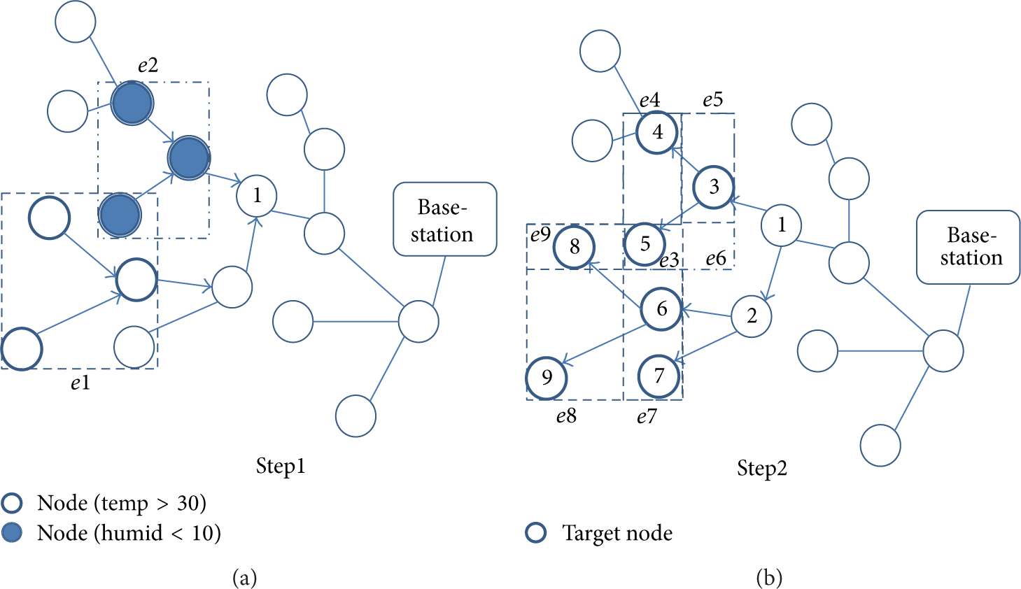
As shown in step 1 of Figure 3, nodes whose subtrees include the given coordinates will receive and register the query of NearBy (10, 10, 20, 20). Thus, the query is passed along node-1 to node-6. On the other hand, node-7 to node-10 do not receive the query since node-5 and node-6 did not send the query because their subtrees do not include the given coordinates. In step 2, node-4 forms ${\mathrm{S}\mathrm{N}\mathrm{Q}\mathrm{L}}^{+s}$   envelope e3 and receives ${\mathrm{S}\mathrm{N}\mathrm{Q}\mathrm{L}}^{+s}$   envelopes e1 and e2 formed by node-5 and node-6, respectively. Then, node-4 passes e1 as the nearest one to the given target location to the base-station.

The procedure of NearBy operation is given in Algorithm 2. This operation receives coord (i.e., coordinates of a target location) as an input and returns a set of geometric space $S_{\mathrm{r}\mathrm{e}\mathrm{s}\mathrm{u}\mathrm{l}\mathrm{t}}=\{e_m\}$ , where $e_m=\{space\text{-}ID,(x_i,x_i,y_i,y_i)\}$ . First, a ${\mathrm{S}\mathrm{N}\mathrm{Q}\mathrm{L}}^{+s}$   envelope $e_N$ is created in a form $〈\mathrm{t}\mathrm{i}\mathrm{m}\mathrm{e}\mathrm{s}\mathrm{t}\mathrm{a}\mathrm{m}\mathrm{p},(x_N,x_N,y_N,y_N)〉$ (line 1). If any envelopes created from $N_{\mathrm{c}\mathrm{h}\mathrm{i}\mathrm{l}\mathrm{d}}$ exist, they are compared with $e_N$ to find the nearest one to coord. Then, the nearest envelope is returned (lines 2–5).

Algorithm 2: Procedure of NearBy operation.

Function   $$Operato{r}_{NearBy}$$

Input: coord = ( $$x_i$$ , $$x_i$$ , $$y_i$$ , $$y_i$$ ) //the specified coordinates of target location

Output:   $$S_{\text{result}}$$ = $$\{e_m\}$$ where $$e_m$$ = {space-ID, ( $$x_i$$ , $$x_i$$ , $$y_i$$ , $$y_i$$ )}

Begin

(1) create $$e_N$$ = $$〈\text{timestamp},(x_N,x_N,y_N,y_N)〉$$

(2) If any envelopes created from $$N_{\text{child}}$$ exits then

(3)  find the nearest envelope to coord among $$e_N$$ and envelopes created from $$N_{\text{child}}$$

(4)  set the nearest envelope to $$S_{\text{result}}$$   End If

(5) return   $$S_{\text{result}}$$

End

3.2.3. Distance (Envelope(s), Range Value)

The Distance operation identifies a geometric space for range value from a designated geometric space. As mentioned in Section 3.1, it is to be noted that a point of location is also expressed as a ${\mathrm{S}\mathrm{N}\mathrm{Q}\mathrm{L}}^{+s}$   envelope. For example, a query: “find the space of sensor nodes which is 10 meter away from the geometric space where the temperature is above 30 degrees” is expressed by Distance (Envelope (temp > 30), 10 m).

As shown in step 1 of Figure 4, node-5 as a LCA node identifies two ${\mathrm{S}\mathrm{N}\mathrm{Q}\mathrm{L}}^{+s}$   envelopes e1 and e2 whose member nodes satisfy the temperature condition. In step 2, node-5 produces expanded ${\mathrm{S}\mathrm{N}\mathrm{Q}\mathrm{L}}^{+s}$   envelopes e1 and e2 according to the given range value and sends the query to expanded ${\mathrm{S}\mathrm{N}\mathrm{Q}\mathrm{L}}^{+s}$   envelopes e1 and e2.

Figure 4

Distance (Envelope (temp > 30), 10 m).

The procedure of the Distance operation is given in Algorithm 3. This function receives a set of geometric spaces $S_{\mathrm{i}\mathrm{n}}=\{e_1,e_2,\dots ,e_k\}$ , where $e_k=\{space\text{-}ID,(x_i,x_j,y_i,y_j)\}$ , and a range value as input. It returns a set of geometric spaces $S_{\mathrm{r}\mathrm{e}\mathrm{s}\mathrm{u}\mathrm{l}\mathrm{t}}=\{{e_1}^{\prime },{e_2}^{\prime },\dots ,{e_k}^{\prime }\}$ , where ${e_k}^{\prime }$ is newly expanded envelope of $e_k$ . To find the new envelope by the range value, each envelope of $e_k$ is expanded by the $(+/-)$ range value given as the second input parameter (lines 1–3). Finally, $S_{\mathrm{r}\mathrm{e}\mathrm{s}\mathrm{u}\mathrm{l}\mathrm{t}}$ is returned (lines 4-5).

Algorithm 3: Procedure of Distance operation.

Function   $$Operato{r}_{Distance}$$

Input: (1) $$S_{\text{in}}$$ = $$\{e_{\mathit{1}}$$ , $$e_{\mathit{2}},\dots ,e_k\}$$ where $$e_k$$ = {space-ID, ( $$x_i$$ , $$x_j$$ , $$y_i$$ , $$y_j$$ )}

   (2) ra // a range value

Output:   $$S_{\text{result}}$$ = $$\{{e_{\mathit{1}}}^{\prime }$$ , $${e_{\mathit{2}}}^{\prime },\dots ,{e_k}^{\prime }\}$$ where $${e_k}^{\prime }$$ is expanded envelope of $$e_k$$

Begin

(1) For each $$e_k$$ in $$S_{\text{in}}$$

(2)   Set envelope of $$e_k$$ with ( $$x_i-\text{ra}$$ , $$x_j+\text{ra}$$ , $$y_i-\text{ra}$$ , $$y_j+\text{ra}$$ )

(3) EndFor

(4) $$S_{\text{result}}:=S_{\text{in}}$$

(5) return   $$S_{\text{result}}$$

End

3.2.4. Direction (Envelope(s), Direction Value)

The Direction operation identifies and returns a geometric space outside designated space in the given directions: NORTH, SOUTH, EAST, WEST, and their mixed orientations as well. For example, a query: “find the space of sensor nodes that are located in the WEST of some space where the temperature is above 30 degrees” is expressed by Direction (Envelope (temp > 30), WEST).

Figure 5 illustrates the operation. In step 1, node-5 as a LCA node identifies ${\mathrm{S}\mathrm{N}\mathrm{Q}\mathrm{L}}^{+s}$   envelopes e1 and e2 whose member nodes have temperature values over 30 degrees. In step 2, node-5 finds e2 as the westernmost envelope of all envelopes and thus returns the ${\mathrm{S}\mathrm{N}\mathrm{Q}\mathrm{L}}^{+s}$   envelope e3 as the result.

Figure 5

Direction (Envelope (temp > 30), WEST).

The procedure of Direction operation is given in Algorithm 4. It receives a set of geometric spaces $S_{\mathrm{i}\mathrm{n}}=\{e_1,e_2,\dots ,e_k\}$ , where $e_k=\{space\text{-}ID,(x_i,x_j,y_i,y_j)\}$ , and a direction value as input. It returns a set of geometric space $S_{\mathrm{r}\mathrm{e}\mathrm{s}\mathrm{u}\mathrm{l}\mathrm{t}}=\{e_m\}$ , where $e_m=\{space\text{-}ID,(x_i,x_j,y_i,y_j)\}$ . After finding the closest envelope to the end of a given direction from $S_{\mathrm{i}\mathrm{n}}$ , the resulting geometric envelope $e_N$ is identified in a given direction D. For example, when the direction is given NORTH, the northernmost envelope in $S_{\mathrm{i}\mathrm{n}}$ will be found and set to ε. Then, envelope $e_N$ with a space coordinates $(X_{\mathrm{m}\mathrm{i}\mathrm{n}},X_{\mathrm{m}\mathrm{a}\mathrm{x}},\epsilon ·y_j,Y_{\mathrm{m}\mathrm{a}\mathrm{x}})$ will be produced as the resulting space whose $y_i$ is greater than $\epsilon ·y_j$ . Here, $X_{\mathrm{m}\mathrm{a}\mathrm{x}}$ ( $X_{\mathrm{m}\mathrm{i}\mathrm{n}}$ ) denotes the maximum (minimum) value of the x-coordinate of the region, and $Y_{\mathrm{m}\mathrm{a}\mathrm{x}}$ ( $Y_{\mathrm{m}\mathrm{i}\mathrm{n}}$ ) denotes the maximum (minimum) value of the y-coordinate of the region (lines 1–14).

Algorithm 4: Procedure of Direction operation.

Function   $$Operato{r}_{Direction}$$

Input: (1) $$S_{\text{in}}$$ = $$\{e_{\mathit{1}}$$ , $$e_{\mathit{2}},\dots ,e_k\}$$ where $$e_k$$ = {space-ID, ( $$x_i$$ , $$x_j$$ , $$y_i$$ , $$y_j$$ )}

     (2) D // a direction value

Output:   $$S_{\text{result}}$$ = $$\{e_m\}$$ where $$e_m$$ = {space-ID, ( $$x_i$$ , $$x_j$$ , $$y_i$$ , $$y_j$$ )}

Begin

(1) Switch(D) // find geometric space of direction operation

(2)   Case ( $$D=\mathit{90}$$ ) or (D = EAST):

(3)     ε $$:=$$ easternmost $$e_k$$ from $$S_{\text{in}}$$

(4)     create $$e_N$$ = $$〈\text{timestamp},(\epsilon \mathrm{\hspace{0.17em}\hspace{0.17em}}·\mathrm{\hspace{0.17em}\hspace{0.17em}}{x}_j,X_{\text{max}},Y_{\text{min}},Y_{\text{max}})〉$$

(5)   Case ( $$D=\mathit{270}$$ ) or (D = WEST):

(6)     ε $$:=$$ westernmost $$e_k$$ from $$S_{\text{in}}$$

(7)     create $$e_N$$ = $$〈\text{timestamp},(X_{\text{min}},\epsilon \mathrm{\hspace{0.17em}\hspace{0.17em}}·\mathrm{\hspace{0.17em}\hspace{0.17em}}{x}_i,Y_{\text{min}},Y_{\text{max}})〉$$

(8)   Case (D = 0) or (D = 360) or (D = NORTH)

(9)     ε $$:=$$ northernmost $$e_k$$ from $$S_{\text{in}}$$

(10)   create $$e_N$$ = $$〈\text{timestamp},(X_{\text{min}},X_{\text{max}},\epsilon \mathrm{\hspace{0.17em}\hspace{0.17em}}·\mathrm{\hspace{0.17em}\hspace{0.17em}}{y}_j,Y_{\text{max}})〉$$

(11)  Case (D = 180) or (D = SOUTH):

(12)    ε $$:=$$ southernmost $$e_k$$ from $$S_{\text{in}}$$

(13)    create $$e_N$$ = $$〈\text{timestamp},(X_{\text{min}},X_{\text{max}},Y_{\text{min}},\epsilon \mathrm{\hspace{0.17em}\hspace{0.17em}}·\mathrm{\hspace{0.17em}\hspace{0.17em}}{y}_i)〉$$

(14) End Switch

(15) $$S_{\text{result}}:=e_N$$

(16) return   $$S_{\text{result}}$$

End

3.3. Set Operators

Set operators are designed to identify the sensor nodes of target spaces by using two operand spaces. With this facility, ${\mathrm{S}\mathrm{N}\mathrm{Q}\mathrm{L}}^{+s}$ allows application programmers to express more sophisticated target region. An example query is “get node IDs from the areas that are designated as multiple spaces where the temperature is above 30°C and/or/but not where the humidity is lower than 10% in the west slope of the mountain.” For that query, Intersection, Union, and Difference operations are used to identify sensor nodes of new spaces. It is noted that Union and Difference operations produce multiple constituent subspaces for the best accuracy of the result as shown in Figure 6. The given spaces are split to subspaces as follows. In step 1, two operand spaces, such as $S_a=\{e_{a1},e_{a2}\}$ and $S_b=\{e_{b1},e_{b2}\}$ , are given. In step 2, after cross product between each element of $S_a$ and that of $S_b$ , intersect envelopes $e_{i1}$ and $e_{i2}$ are identified. In step 3, each element envelopes of $S_a$ and $S_b$ are compared whether the spaces exist surrounding $e_{i1}$ and $e_{i2}$ in the 8 direction: NORTH, SOUTH, EAST, WEST, and their mixed orientations. Then existing spaces form as $S_a=\{e_{s11},e_{s12},e_{s13},e_{s23},e_{s24},e_{s25}\}$ and $S_b=\{e_{s15},e_{s16},e_{s17},e_{s21},e_{s27},e_{s28}\}$ .

Figure 6

Procedure of producing multiple constituent subspaces.

3.3.1. Intersection ((s1, s2)∣Envelope(s), Envelope(s))

The Intersection operation takes two operand spaces either explicitly specified by space-IDs or implicitly specified by two return values (i.e., ${\mathrm{S}\mathrm{N}\mathrm{Q}\mathrm{L}}^{+s}$ envelopes) of spatial operations. For the demonstration purpose we use an example query: “get node IDs from the intersection areas between where the temperature is above 30°C and where the humidity is below 10% in the west slope of the mountain.” This query implies the possible executions for the multiple pairs of overlapping subspaces that satisfy the given conditions and thus a set of subspaces (i.e., ${\mathrm{S}\mathrm{N}\mathrm{Q}\mathrm{L}}^{+s}$   envelopes) will be returned. Figure 7 illustrates an execution of Intersection operation. In step 1, node-1 as a LCA node receives ${\mathrm{S}\mathrm{N}\mathrm{Q}\mathrm{L}}^{+s}$   envelope e1 where the temperature is over 30°C and ${\mathrm{S}\mathrm{N}\mathrm{Q}\mathrm{L}}^{+s}$   envelope e2 where the humidity is below 10%. In step 2, node-1 computes the intersect region of e1 and e2. Then, it creates an ${\mathrm{S}\mathrm{N}\mathrm{Q}\mathrm{L}}^{+s}$   envelope e3 and sends the query to the nodes of e3.

Figure 7

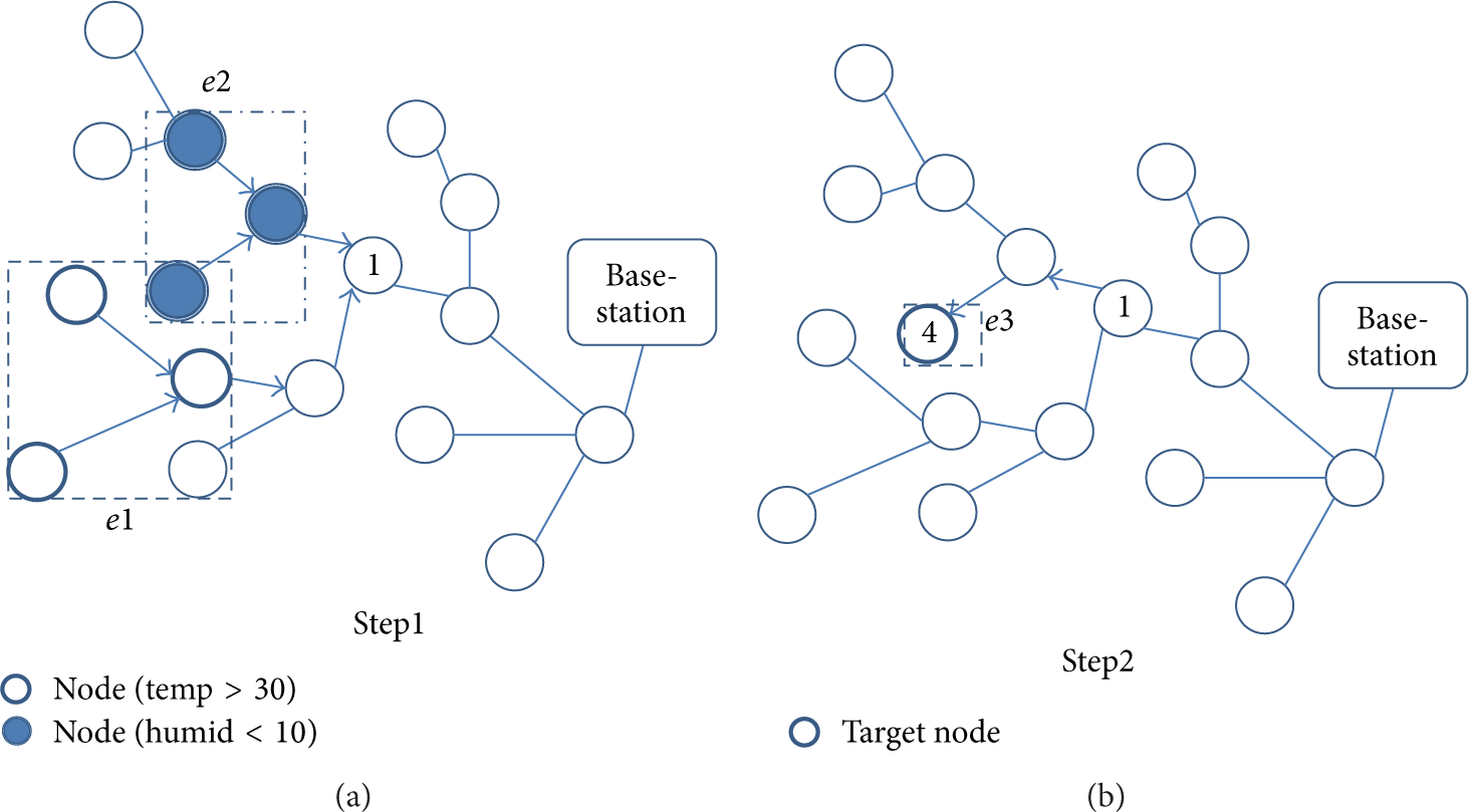
Intersection (Envelope (temp > 30), Envelope (humid < 10)).

3.3.2. Union ((s1, s2)∣Envelope(s), Envelope(s))

The Union operation takes two operand spaces either explicitly specified by space-IDs or implicitly specified by two return values (i.e., ${\mathrm{S}\mathrm{N}\mathrm{Q}\mathrm{L}}^{+s}$ envelopes) of spatial operations. An example query: “get node IDs from the union areas where the temperature is above 30°C or where the humidity is below 10% in the west slope of the mountain” is used. This example implies the possible execution of the multiple pairs of overlapping subspaces that satisfy the given conditions and, as the result, a set of constituent subspaces (i.e., ${\mathrm{S}\mathrm{N}\mathrm{Q}\mathrm{L}}^{+s}$   envelopes) will be returned. Figure 8 illustrates an example execution of the Union operation. In step 1, node-1 as a LCA node receives ${\mathrm{S}\mathrm{N}\mathrm{Q}\mathrm{L}}^{+s}$   envelope e1 where the temperature is over 30°C and ${\mathrm{S}\mathrm{N}\mathrm{Q}\mathrm{L}}^{+s}$   envelope e2 where the humidity is below 10%. In step 2, node-1 computes the union area of e1 and e2 by splitting it based on the intersect area. Then, it creates e3 to e9 and sends the query to the sensor nodes of e3 to e9. It is to be noted that, unlike the Intersection operation, the Union operation yields a set of constituent envelopes that together form the union of two spaces as shown in Figure 8 (step 2).

Figure 8

Union (Envelope (temp > 30), Envelope (humid < 10)).

3.3.3. Difference ((s1, s2)∣Envelope(s), Envelope(s))

The Difference operation takes two operand spaces either explicitly specified by space-IDs or implicitly specified by two return values (i.e., ${\mathrm{S}\mathrm{N}\mathrm{Q}\mathrm{L}}^{+s}$   envelopes) of spatial operations. An example query: “get node IDs from the areas where the temperature is above 30°C but where the humidity is not below 10% in the west slope of the mountain” is used. This example implies the possible execution of multiple pairs of overlapping spaces that satisfy the given conditions and, as the result, a set of constituent subspaces (i.e., ${\mathrm{S}\mathrm{N}\mathrm{Q}\mathrm{L}}^{+s}$   envelopes) will be returned. Figure 9 illustrates an example execution of the Difference operation. In step 1, node-1 as a LCA node receives ${\mathrm{S}\mathrm{N}\mathrm{Q}\mathrm{L}}^{+s}$   envelope e1 where the temperature is over 30°C and ${\mathrm{S}\mathrm{N}\mathrm{Q}\mathrm{L}}^{+s}$   envelope e2 where the humidity is below 10%. In step 2, node-1 computes the area of difference between e1 and e2 by splitting it based on the common area. Then, it creates ${\mathrm{S}\mathrm{N}\mathrm{Q}\mathrm{L}}^{+s}$   envelopes e3, e4, and e5 and sends the query to nodes in e3, e4, and e5. Similar to the Union operation, this operation yields a set of constituent envelopes that together form the resulting subspaces of the Difference operation as shown in Figure 9 (step 2).

Figure 9

Difference (Envelope (temp > 30), Envelope (humid < 10)).

The procedure of Set operation is given in Algorithm 5. This function receives op_name (i.e., operator name), $S_a=\{e_1,e_2,\dots ,e_a\}$ and $S_b=\{e_1,e_2,\dots ,e_b\}$ as input, and it returns a set of geometric spaces $S_{\mathrm{r}\mathrm{e}\mathrm{s}\mathrm{u}\mathrm{l}\mathrm{t}}=\left\{e_1,e_2,\dots ,e_n\right\}$ , where $e_n=\{space\text{-}ID,(x_i,x_j,y_i,y_j)\}$ . First, when each envelope $e_a$ in $S_a$ overlaps with envelope $e_b$ in $S_b$ , an intersect envelope $e_i$ is created in a form $〈\mathrm{t}\mathrm{i}\mathrm{m}\mathrm{e}\mathrm{s}\mathrm{t}\mathrm{a}\mathrm{m}\mathrm{p},(x_i,x_j,y_i,y_j)〉$ (lines 1–4). By comparing it in 8 directions (i.e., NORTH, SOUTH, EAST, WEST, and their mixed orientations), $e_a$ is split into each direction-positioned constituent envelope when if $e_a$ exists next to $e_i$ on each direction. Then, those envelopes form ${\epsilon }_a=\{e_1,e_2,\dots ,e_k\}$ . Also, $e_b$ is split in the same manner. Here, the constituent envelopes are identified by the position of $e_i$ . In the case of Figure 8, $e_3$ is created as an intersecting envelope and then ${\epsilon }_a=\{e_7,e_8,e_9\}$ and ${\epsilon }_b=\{e_4,e_5,e_6\}$ are created surrounding $e_3$ , whereas envelopes are not created in the positions of north-west and south-east from $e_3$ (lines 5-6). If op_name is “Intersection,” $e_i$ is added to $S_{\mathrm{r}\mathrm{e}\mathrm{s}\mathrm{u}\mathrm{l}\mathrm{t}}$ (line 7). If op_name is “Difference,” ${\epsilon }_a$ is added to $S_{\mathrm{r}\mathrm{e}\mathrm{s}\mathrm{u}\mathrm{l}\mathrm{t}}$ (line 8). If op_name is “Union,” ${\epsilon }_a$ , ${\epsilon }_b$ , and $e_i$ are added to $S_{\mathrm{r}\mathrm{e}\mathrm{s}\mathrm{u}\mathrm{l}\mathrm{t}}$ (line 9). If overlap does not exist, $e_a$ is added to $S_{\mathrm{r}\mathrm{e}\mathrm{s}\mathrm{u}\mathrm{l}\mathrm{t}}$ when the op_name is “Difference.” Otherwise, $e_a$ and $e_b$ are added to $S_{\mathrm{r}\mathrm{e}\mathrm{s}\mathrm{u}\mathrm{l}\mathrm{t}}$ when the op_name is “Union” (lines 10–12). Finally, redundant envelopes, caused from cross product between $S_a$ and $S_b$ , are removed from $S_{\mathrm{r}\mathrm{e}\mathrm{s}\mathrm{u}\mathrm{l}\mathrm{t}}$ (line 16). Table 1 summarizes the spatial operators in ${\mathrm{S}\mathrm{N}\mathrm{Q}\mathrm{L}}^{+s}$ .

Table 1

Spatial operators in SNQL^+s.

Division	Operator	Description
Space identification operators	Envelope	Return the geometric spaces that satisfy a given condition
	NearBy	Return the geometric space that is the nearest to the specified point of location
	Distance	Return the geometric spaces that satisfy within the given distance from the given geometric spaces
	Direction	Return the geometric space that satisfies the given direction from the given geometric spaces
Set operators	Intersection	Return the geometric spaces that lie in the intersection area of the given geometric spaces
	Union	Return the geometric spaces that lie in the union area of the given geometric spaces
	Difference	Return the geometric spaces that lie in the difference area of the given geometric spaces

Algorithm 5: Procedure of SetOperators operation.

Function   $$Operato{r}_{SetOperators}$$

Input: (1) op_name

   (2) $$S_a$$ = $$\{e_{\mathit{1}}$$ , $$e_{\mathit{2}},\dots ,e_a\}$$ where $$e_a$$ = {space-ID, ( $$x_i$$ , $$x_j$$ , $$y_i$$ , $$y_j$$ )}

   (3) $$S_b$$ = $$\{e_{\mathit{1}}$$ , $$e_{\mathit{2}},\dots ,e_b\}$$ where $$e_b$$ = {space-ID, ( $$x_i$$ , $$x_j$$ , $$y_i$$ , $$y_j$$ )}

Output:   $$S_{\text{result}}$$ = $$\{e_{\mathit{1}}$$ , $$e_{\mathit{2}},\dots ,e_n\}$$ where $$e_n$$ = {space-ID, ( $$x_i$$ , $$x_j$$ , $$y_i$$ , $$y_j$$ )}

Begin

(1)    For each $$e_a$$ in $$S_a$$

(2)     For each $$e_b$$ in $$S_b$$

(3)     If envelope of $$e_a$$ overlap that of $$e_b$$   then

(4)       create intersect envelope $$e_i$$ = $$〈\text{timestamp},(x_i,x_j,y_i,y_j)〉$$

(5)       create $${\epsilon }_a$$ = $$\{e_{\mathit{1}}$$ , $$e_{\mathit{2}},\dots ,e_k\}$$ where $$e_k$$ is constituent envelope of $$e_a$$ by splitting $$e_a$$ surrounding $$e_i$$

(6)       create $${\epsilon }_b$$ = $$\{e_{\mathit{1}}$$ , $$e_{\mathit{2}},\dots ,e_k\}$$ where $$e_k$$ is constituent envelope of $$e_b$$ by splitting $$e_b$$ surrounding $$e_i$$

(7)       If (op_name = “Intersection”) then add $$e_i$$ to $$S_{\text{result}}$$   End If

(8)       If (op_name = “Difference”) then add $${\epsilon }_a$$ to $$S_{\text{result}}$$   End If

(9)       If (op_name = “Union”) then add $${\epsilon }_a$$ , $${\epsilon }_b$$ , $$e_i$$ to $$S_{\text{result}}$$   End If

(10)  Else

(11)     If (op_name = “Difference”) then add $$e_a$$ to $$S_{\text{result}}$$   End If

(12)    If (op_name = “Union”) then add $$e_a$$ , $$e_b$$ to $$S_{\text{result}}$$   End If

(13)  End If

(14)   EndFor

(15) EndFor

(16) remove redundant envelopes from $$S_{\text{result}}$$

(17) return   $$S_{\text{result}}$$

End

3.4. Spatial Expressions in ${\text{SNQL}}^{+\mathit{s}}$

In this section, ${\mathrm{S}\mathrm{N}\mathrm{Q}\mathrm{L}}^{+s}$   is introduced, which extends SNQL (Sensor Network Query Language) [8, 14] to be able to support the spatial operators. The original SNQL was designed based on SELECT-FROM-WHERE structure and supports instant queries, continuous queries, and event-based queries. Algorithm 6 shows the basic structure of the original SNQL. SELECT-clause describes the attributes that correspond to the data to be collected from each sensor node. FROM-clause specifies the initial target space for query dissemination. WHERE-clause describes the selection condition(s). EVENT ON specifies predefined events for the following query to be executed when the event takes place. SAMPLE PERIOD specifies various temporal notations for data collection. OUTPUT ACTION defines the sensor action to be performed when event or selection condition(s) are met. WITHIN-clause specifies the percentage of the nodes out of all the participating sensor nodes in the query processing, and CASE WHEN allows branching of query actions according to the situational conditions. More details are referred to in [8, 14].

Algorithm 6: The structure of SNQL.

EVENT  ON   event-type (paramlist)

SELECT   selectlist

FROM   fromlist

WHERE  expression

SAMPLE  PERIOD  time [FOR  time]

OUTPUT  ACTION   command

WITHIN   percentage

CASE  WHEN  event ∣ expression

 THEN  Action ∣ Sample Period ∣ Within

END;

To add spatial operators to the SNQL [8, 14], the expression in the WHERE-clause and WHEN-clause is extended as described in Algorithm 7. More specifically, <SpatialFunc> is added to <SQLSimpleExp> of <Expression> so that the spatial operators previously explained can be used. <SpatialFunc> consists of <Envelope>, <NearBy>, <Distance>, <Direction>, <Intersection>, <Union>, and <Difference>. <Envelope> is expressed as a combination of attributes (e.g., temperature), operators (e.g., “>”, “<”, or “=”), and constants. <NearBy> is expressed as integer values representing the coordinates x and y. <Distance> expresses the operator selected from the elements of <SpatialFunc> and a constant indicating the distance. <Direction> expresses the operator selected from the elements of <SpatialFunc> and a constant indicating the direction. <Intersection> consists of combinations of <SpatialFunc> entities used to obtain the intersection. <Union> consists of combinations of <SpatialFunc> entities used to obtain the union area. <Difference> consists of combinations of <SpatialFunc> entities used to obtain the difference area. <envelope>, <attribute>, <operator>, and <constant> are fundamental attributes, whose descriptions are thus not necessary.

Algorithm 7: Spatial expression in SNQL^+s.

$$〈\mathbf{E}\mathbf{x}\mathbf{p}\mathbf{r}\mathbf{e}\mathbf{s}\mathbf{s}\mathbf{i}\mathbf{o}\mathbf{n}〉$$ ::= $$〈\text{SQLAndExp}〉$$ (“OR” $$〈\text{SQLAndExp}〉$$ )

$$〈\mathbf{S}\mathbf{Q}\mathbf{L}\mathbf{A}\mathbf{n}\mathbf{d}\mathbf{E}\mathbf{x}\mathbf{p}〉$$ ::= $$〈\text{SQLRelationalExp}〉$$ (“AND” $$〈\text{SQLRelationalExp}〉$$ )

$$〈\mathbf{S}\mathbf{Q}\mathbf{L}\mathbf{R}\mathbf{e}\mathbf{l}\mathbf{a}\mathbf{t}\mathbf{i}\mathbf{o}\mathbf{n}\mathbf{a}\mathbf{l}\mathbf{E}\mathbf{x}\mathbf{p}〉$$ ::= $$〈\text{SQLSimpleExp}〉$$   ∣   $$〈\text{SQLExpressionList}〉$$   ∣   $$〈\text{SQLInClause}〉$$   ∣   $$〈\text{SQLBetweenClause}〉$$

$$〈\mathbf{S}\mathbf{Q}\mathbf{L}\mathbf{E}\mathbf{x}\mathbf{p}\mathbf{r}\mathbf{e}\mathbf{s}\mathbf{s}\mathbf{i}\mathbf{o}\mathbf{n}\mathbf{L}\mathbf{i}\mathbf{s}\mathbf{t}〉$$ ::= $$〈\text{SQLSimpleExp}〉$$ (“,” $$〈\text{SQLSimpleExp}〉$$ )

$$〈\mathbf{S}\mathbf{Q}\mathbf{L}\mathbf{S}\mathbf{i}\mathbf{m}\mathbf{p}\mathbf{l}\mathbf{e}\mathbf{E}\mathbf{x}\mathbf{p}〉$$ ::= $$〈\text{AggregateFunc}〉$$   ∣   $$〈\text{Count}〉$$   ∣   $$〈\text{NUMBER}〉$$   ∣   $$〈\text{STRING}〉$$   ∣   $$〈\text{BIND}〉$$   ∣   $$〈\mathbf{S}\mathbf{p}\mathbf{a}\mathbf{t}\mathbf{i}\mathbf{a}\mathbf{l}\mathbf{F}\mathbf{u}\mathbf{n}\mathbf{c}〉$$

$$〈\mathbf{S}\mathbf{p}\mathbf{a}\mathbf{t}\mathbf{i}\mathbf{a}\mathbf{l}\mathbf{F}\mathbf{u}\mathbf{n}\mathbf{c}〉$$ ::= $$〈\text{Envelope}〉$$   ∣   $$〈\text{Nearby}〉$$   ∣   $$〈\text{Intersection}〉$$   ∣   $$〈\text{Union}〉$$   ∣   $$〈\text{Difference}〉$$   ∣   $$〈\text{Distance}〉$$   ∣   $$〈\text{Direction}〉$$

$$〈\mathbf{E}\mathbf{n}\mathbf{v}\mathbf{e}\mathbf{l}\mathbf{o}\mathbf{p}\mathbf{e}〉$$ ::=“ENVELOPE (“ $$〈\text{attribute}〉〈\text{operator}〉〈\text{constant}〉$$ ”)”

$$〈\mathbf{N}\mathbf{e}\mathbf{a}\mathbf{r}\mathbf{B}\mathbf{y}〉$$ ::=“NEARBY (“ $$〈\text{envelope}〉$$ ”)”

$$〈\mathbf{I}\mathbf{n}\mathbf{t}\mathbf{e}\mathbf{r}\mathbf{s}\mathbf{e}\mathbf{c}\mathbf{t}\mathbf{i}\mathbf{o}\mathbf{n}〉$$ ::=“INTERSECTION (” $$〈\text{SpatialFunc}〉$$ “,” $$〈\text{SpatialFunc}〉$$ “)”

$$〈\mathbf{U}\mathbf{n}\mathbf{i}\mathbf{o}\mathbf{n}〉$$ ::=“UNION (” $$〈\text{SpatialFunc}〉$$ “,” $$〈\text{SpatialFunc}〉$$ “)”

$$〈\mathbf{D}\mathbf{i}\mathbf{f}\mathbf{f}\mathbf{e}\mathbf{r}\mathbf{e}\mathbf{n}\mathbf{c}\mathbf{e}〉$$ ::=“DIFFERENCE (” $$〈\text{SpatialFunc}〉$$ “,” $$〈\text{SpatialFunc}〉$$ “)”

$$〈\mathbf{D}\mathbf{i}\mathbf{s}\mathbf{t}\mathbf{a}\mathbf{n}\mathbf{c}\mathbf{e}〉$$ ::=“DISTNACE (” $$〈\text{SpatialFunc}〉$$ “,” $$〈\text{constant}〉$$ “)”

$$〈\mathbf{D}\mathbf{i}\mathbf{r}\mathbf{e}\mathbf{c}\mathbf{t}\mathbf{i}\mathbf{o}\mathbf{n}〉$$ ::=“DIRECTION (” $$〈\text{SpatialFunc}〉$$ “,” $$〈\text{constant}〉$$ “)”

$$〈\mathbf{e}\mathbf{n}\mathbf{v}\mathbf{e}\mathbf{l}\mathbf{o}\mathbf{p}\mathbf{e}〉$$ ::=“(” $$〈\text{integer}〉$$ “,” $$〈\text{integer}〉$$ “,” $$〈\text{integer}〉$$ “,” $$〈\text{integer}〉$$ “)”

$$〈\mathbf{a}\mathbf{t}\mathbf{t}\mathbf{r}\mathbf{i}\mathbf{b}\mathbf{u}\mathbf{t}\mathbf{e}〉$$ ::= $$〈\text{string}〉$$

$$〈\mathbf{o}\mathbf{p}\mathbf{e}\mathbf{r}\mathbf{a}\mathbf{t}\mathbf{o}\mathbf{r}〉$$ ::=“>” ∣ “<” ∣ “=” ∣ “<>” ∣ “>=” ∣ “<=”

$$〈\mathbf{c}\mathbf{o}\mathbf{n}\mathbf{s}\mathbf{t}\mathbf{a}\mathbf{n}\mathbf{t}〉$$ ::= $$〈\text{integer}〉$$   ∣   $$〈\text{float}〉$$   ∣   $$〈\text{string}〉$$

4. LCA: In-Network Query Processing Algorithm

Sensor network queries often involve multiple phases of data reading in a single query task. The example query given in Section 1 “read the temperatures from the regions where the humidity is lower than 10% in the west slope of the mountain” involves two separate tasks: (1) read the humidity values from all the nodes in the west slope and (2) read the temperature values from the nodes in spaces where the humidity values are below 10%. In the existing systems, this operation would require two traversals between the base-station and the target nodes of the designated spaces.

Our proposed query processing algorithm enables the multiple phases of querying tasks to be handled by an in-network node called lowest common ancestor (LCA) node. The LCA node is one of the intermediate parent nodes which distributes the query to more than two child nodes for the first time and minimally covers all the child nodes of the target space. It has been designed to play the role of in-network query reformation and redissemination for the multiple reading tasks. This query processing algorithm will efficiently reduce the energy consumption of wireless sensor nodes incurred by unnecessary transmissions of multiple queries/data between the base-station (i.e., root node) and the target nodes.

The procedure of finding the LCA node is as follows. Each node along the query path manages two parameters ( $\#{\mathrm{A}\mathrm{n}\mathrm{c}\mathrm{e}\mathrm{s}\mathrm{t}\mathrm{o}\mathrm{r}}_{\mathrm{m}\mathrm{a}\mathrm{x}\_\mathrm{s}\mathrm{e}\mathrm{n}\mathrm{d}}$ , $\#{\mathrm{C}\mathrm{h}\mathrm{i}\mathrm{l}\mathrm{d}}_{\mathrm{s}\mathrm{e}\mathrm{n}\mathrm{d}}$ ). The former describes the maximum number of child nodes to which its ancestor nodes send the query, and the latter describes the number of child nodes to which it passes the query further. The LCA node is identified for a node when its $\#{\mathrm{C}\mathrm{h}\mathrm{i}\mathrm{l}\mathrm{d}}_{\mathrm{s}\mathrm{e}\mathrm{n}\mathrm{d}}$ value becomes greater than 1 for the first time along the query path.

Figure 10(a) illustrates how a LCA node is determined for the example query to the first target space. N01, as the base-station, receives the query and the Planner of Query Processor finds N02 as the receiver node toward the target space. Here, since N01 does not have a parent, $\#{\mathrm{A}\mathrm{n}\mathrm{c}\mathrm{e}\mathrm{s}\mathrm{t}\mathrm{o}\mathrm{r}}_{\mathrm{m}\mathrm{a}\mathrm{x}\_\mathrm{s}\mathrm{e}\mathrm{n}\mathrm{d}}$ becomes 0. And, as it passes the query only to N02, $\#{\mathrm{C}\mathrm{h}\mathrm{i}\mathrm{l}\mathrm{d}}_{\mathrm{s}\mathrm{e}\mathrm{n}\mathrm{d}}$ becomes 1. In this manner, N03, N04, N05, and N06 positioned in the query path to the first target will have ( $\#{\mathrm{A}\mathrm{n}\mathrm{c}\mathrm{e}\mathrm{s}\mathrm{t}\mathrm{o}\mathrm{r}}_{\mathrm{m}\mathrm{a}\mathrm{x}\_\mathrm{s}\mathrm{e}\mathrm{n}\mathrm{d}}=1$ , $\#{\mathrm{C}\mathrm{h}\mathrm{i}\mathrm{l}\mathrm{d}}_{\mathrm{s}\mathrm{e}\mathrm{n}\mathrm{d}}=1$ ). N07 receives the query from N06 and passes the query down to two child nodes so that the number of child nodes, for the first time, becomes greater than 1 that is ( $\#{\mathrm{A}\mathrm{n}\mathrm{c}\mathrm{e}\mathrm{s}\mathrm{t}\mathrm{o}\mathrm{r}}_{\mathrm{m}\mathrm{a}\mathrm{x}\_\mathrm{s}\mathrm{e}\mathrm{n}\mathrm{d}}=1$ , $\#{\mathrm{C}\mathrm{h}\mathrm{i}\mathrm{l}\mathrm{d}}_{\mathrm{s}\mathrm{e}\mathrm{n}\mathrm{d}}=2$ ). Therefore, N07 becomes the LCA node for the query, which is the lowest intermediate node that minimally covers all nodes of the target space (i.e., the west slope).

Figure 10

In-network query process with LCA node.

In Figure 10(b), the LCA node carries out a query task for data collection from the final target nodes (i.e., the nodes with humidity values lower than 10% within the initial target space). For this, the LCA node plays the key role of identifying the final target nodes and redisseminates the subsequent query task to the nodes (i.e., temperature reading).

The procedure of LCA operation is given in Algorithm 8. This function receives $\#{\mathrm{A}\mathrm{n}\mathrm{c}\mathrm{e}\mathrm{s}\mathrm{t}\mathrm{o}\mathrm{r}}_{\mathrm{m}\mathrm{a}\mathrm{x}\_\mathrm{s}\mathrm{e}\mathrm{n}\mathrm{d}}$ and $\#{\mathrm{C}\mathrm{h}\mathrm{i}\mathrm{l}\mathrm{d}}_{\mathrm{s}\mathrm{e}\mathrm{n}\mathrm{d}}$ as the input and returns True or False according to decision whether current node is LCA node or not. First, the registered query is reformed with envelopes received from its child nodes, if the current node satisfies following conditions: (1) for nodes ( $\#{\mathrm{A}\mathrm{n}\mathrm{c}\mathrm{e}\mathrm{s}\mathrm{t}\mathrm{o}\mathrm{r}}_{\mathrm{m}\mathrm{a}\mathrm{x}\_\mathrm{s}\mathrm{e}\mathrm{n}\mathrm{d}}=1$ , $\#{\mathrm{C}\mathrm{h}\mathrm{i}\mathrm{l}\mathrm{d}}_{\mathrm{s}\mathrm{e}\mathrm{n}\mathrm{d}}>1$ ) and (2) for base-station ( $\#{\mathrm{A}\mathrm{n}\mathrm{c}\mathrm{e}\mathrm{s}\mathrm{t}\mathrm{o}\mathrm{r}}_{\mathrm{m}\mathrm{a}\mathrm{x}\_\mathrm{s}\mathrm{e}\mathrm{n}\mathrm{d}}=0$ , $\#{\mathrm{C}\mathrm{h}\mathrm{i}\mathrm{l}\mathrm{d}}_{\mathrm{s}\mathrm{e}\mathrm{n}\mathrm{d}}>1$ ) (lines 1-2). Then, the Planner of Query Processor (or Disseminator) is called to disseminate the reformed query. And, true is returned (lines 3–5). If current node is not LCA node, false is returned (line 6).

Algorithm 8: Procedure of LCA operation.

Function   LCA

Input: (1) # $$\text{Ancesto}{\text{r}}_{\text{max\_send}}$$

   (2) # $$\text{Chil}{\text{d}}_{\text{send}}$$

Output: a Boolean value // true or false

Begin

(1) If ((# $$\text{Ancesto}{\text{r}}_{\text{max\_send}}$$ = 1 and # $$\text{Chil}{\text{d}}_{\text{send}}$$ > 1)

  ∣∣ (# $$\text{Ancesto}{\text{r}}_{\text{max\_send}}$$ = 0 and # $$\text{Chil}{\text{d}}_{\text{send}}$$ > 1)) then

(2) reform the registered query with envelopes receive from child nodes

(3) If the current node is base-station then call the Planner of Query Processor

(4) Else call the Disseminator End If

(5) return true

(6) Else return false  End If

End

5. Architecture

5.1. Overview

This section describes the architecture of our sensor network database system. It consists of functional components of the base-station as the ${\mathrm{S}\mathrm{N}\mathrm{Q}\mathrm{L}}^{+s}$ server and sensor nodes as illustrated in Figure 11. Upon receiving a query, the Query Processor parses the query, plans execution, and sends the parsed query out to the network manager. It uses the metadata about the nodes and their connectivity (i.e., topology) to determine the pathway to the target nodes. The nodes along the hierarchical pathway to the sensor nodes of the initial target region will register the parsed query as the ancestor nodes for the target nodes, and one of the nodes will play the LCA role for identifying the new target nodes when multiple space operations apply. The executors of the nodes in the target space execute the query and return the data toward the ${\mathrm{S}\mathrm{N}\mathrm{Q}\mathrm{L}}^{+s}$ server along the ancestor nodes. The Event Manager at the sensor node manages the events query registered at the target nodes, and the Action Manager manages the actions (e.g., beeping, beckoning, etc.) that need to be executed when the query condition is satisfied. The Network Manager passes the parsed query down to the nodes of the target region, receives the query result, and returns them to its parent node. Finally, the base-station postprocesses the collected sensor data into a form requested by the given query before giving them out to the application.

Figure 11

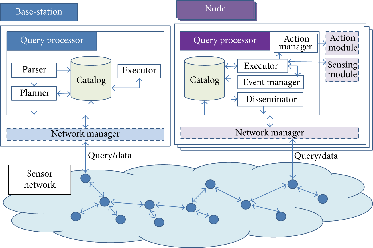
System architecture of sensor network database using ${\mathrm{S}\mathrm{N}\mathrm{Q}\mathrm{L}}^{+s}$ .

5.2. Metadata Management

The metadata of ${\mathrm{S}\mathrm{N}\mathrm{Q}\mathrm{L}}^{+s}$ , such as attribute types, location information, and minimum boundary rectangle (MBR) of sensor nodes are used during the query processing. Each node manages the metadata of directly connected child nodes in the form: $\{(x_i,y_i),(NodeID,\{sensorType\})\}$ , where $(x_i,y_i)$ denotes the coordinates of its child nodes and $(NodeID,\{sensorType\})$ denotes their nodeIDs and sensor types. Also, the metadata of its subtrees are described in the form: $\{(x_i,x_j,y_i,y_j),\{sensorType\}\}$ , where $(x_i,x_j,y_i,y_j)$ denotes the vertices as its MBR and $\{sensorType\}$ denotes sensor types of nodes in the subtree. Figure 12 shows an example of metadata management. Circles indicate sensor nodes, and the dotted line represents the region of the subtree as a MBR. The base-station manages “ $〈(\mathrm{10,60}),(N01,\left\{sensorType\right\})〉$ ” as the metadata of the directly connected node and “ $〈(10,50,40,100),\{sensorType\}〉$ ” as the metadata of its subtree. Also, senor node N01 manages “ $〈((25,95),(N02,\{sensorType\}))$ , $((22,58)$ , $(N03,\{sensorType\}))〉$ ” as metadata of the directly connected child nodes and “ $〈((25,45,77,100)$ , $\{sensorType\})$ , $(\left(22,50,40,58\right),\left\{sensorType\right\})〉$ ” as the metadata of its subtrees. In this manner, N02 manages the metadata of the directly connected two child nodes and two subtrees including MBR. Here, the MBR of subtree is used for determining to pass the query down to the child nodes when the target space overlaps MBR of subtrees. This metadata is created at the time of construction of the sensor network. When a node is added or deleted, the metadata is reconstructed by updating its parent and child nodes.

Figure 12

An example of managing metadata.

6. Performance Evaluation

6.1. Test Data and Environment

In this section, the performance of our proposed spatial query processing strategy is evaluated based on the energy efficiency. We used the Intel Berkeley Research lab data [22] to generate random sensing data as follows: normal distributions with a mean of 22.07 and a standard deviation of 3.662 for temperature data; a mean of 39.29 and a standard deviation of 7.162 for humidity data; and a mean of 390.87 and a standard deviation of 534.39 for illumination data. The number of nodes is set to 10000, and the sampling count of each node is set to 1000. Energy consumption of sensor network is caused by transmission, reception, processing, and sensing of queries and data [9]. Table 2 summarizes the simulation parameters.

Table 2

Simulation parameters.

Type	Parameter	Value
Network and nodes	Number of nodes	10,000
	Sampling count of each node	1,000
	Network range	1,000 m * 1,000 m
	Time to sensing (s)	1
	Network topology	Tree
	Transmit energy (mA)	10.40
	Receive energy (mA)	9.30
Energy consumption [9]	Processor, active (mA)	5.00
	Processor, idle (mA)	0.001
	Sensing energy (mA)	0.5

All the experiments were conducted with a simulator which was programmed internally in Java and was extended version of our previous work [8, 14, 23].

6.2. Experiments and Results

The efficiency of LCA-based spatial operations is evaluated by two experiments for two typical spatial operations of multiple targeting: operation for identifying intermediate target region and operation for targeting multiple regions, respectively.

Experiment 1. A test query for identifying a new target region according to the data result from the initial target space.

In this experiment, we measured the amount of energy consumption for two different query processing methods: one with LCA-based spatial operation and the other without the operation. This is measured by varying the distance of target region from the base-station as shown in Figure 13.

Figure 13

Area of target nodes varying the position of region.

The query used for this experiment is as follows.

“Get NodeID and light value of nodes from the intersecting area between an area with temperature above T°C and another area with the humidity below H% within the area of $(x_1,x_2,y_1,y_2)$ .”

The above query is expressed in ${\mathrm{S}\mathrm{N}\mathrm{Q}\mathrm{L}}^{+s}$ as follows:

•  

SELECT NodeID, light

 

FROM sensors

 

WHERE $s_1(x_1,x_2,y_1,y_2)$

 

AND Intersection (Envelope (temp > T°C), Envelope (humid < H%))

Multiple queries are needed when spatial operations with LCA algorithm are not supported as in SNQL [8, 14] as follows:

•  

① SELECT NodeID, x, y FROM sensors WHERE $x\ge x_1$ AND $x\le x_2$ AND $y\ge y_1$ AND $y\le y_2$ AND (temp > T°C)

 

②  SELECT NodeID, x, y FROM sensors WHERE $x\ge x_1$ AND $x\le x_2$ AND $y\ge y_1$ AND $y\le y_2$ AND (humid < H%)

 

③ SELECT NodeID, light FROM sensors WHERE $x\ge x_{11}$ AND $x\le x_{22}$ AND $y\ge y_{11}$ AND $y\le y_{22}$

The base-station will calculate the intersecting areas from the results of query ① and query ② and then obtains the NodeID and light value from query ③.

The multiple query executions to identify intermediate target regions and the extra spatial operation (i.e., INTERSECT) at the base-station will consume energy and give application designer an extra programming overhead. On the other hand, ${\mathrm{S}\mathrm{N}\mathrm{Q}\mathrm{L}}^{+s}$ uses sophisticated spatial expressions in a single query and executes the spatial operations using the LCA algorithm. This will greatly improve energy efficiency and programming convenience.

Figure 14 shows the result of the experiment. Obviously, as the distance of target region from the base-station increased, the number of intermediate nodes to send the final query results to the base-station also increased. Moreover, the gap of energy consumption between two curves becomes larger as our spatial operators with LCA-based processing algorithm effectively reduce multiple query/data transmissions between the base-station and querying nodes.

Figure 14

Varying the position of target region.

Experiment 2. A test query for identifying multiple target regions.

In this experiment, we observe the amount of energy consumption by varying the number of target regions (denoted by the number of target regions: $N_{\mathrm{r}\mathrm{e}\mathrm{g}\mathrm{i}\mathrm{o}\mathrm{n}}$ ) and the ratio of participating nodes in the resulting target region (denoted by selectivity: $N_{\mathrm{s}\mathrm{e}\mathrm{l}\mathrm{e}\mathrm{c}\mathrm{t}}$ ).

The query used for this experiment is as follows.

“Get NodeID and light value of nodes in the area of $(x_{a1},x_{a2},y_{a1},y_{a2})$ or the area of $(x_{b1},x_{b2},y_{b1},y_{b2})$ .”

Multiple queries are needed when spatial operators with LCA-based query processing algorithm are not supported as in SNQL [8, 14] as follows:

•  

① SELECT NodeID, light FROM sensors WHERE $x\ge x_{a1}$ AND $x\le x_{a2}$ AND $y\ge y_{a1}$ AND $y\le y_{a2}$

 

② SELECT NodeID, light FROM sensors WHERE $x\ge x_{b1}$ AND $x\le x_{b2}$ AND $y\ge y_{b1}$ AND $y\le y_{b2}$

The multiple query executions in sending the queries to multiple target regions will consume energy and give application designer an extra programming overhead.

The above query is expressed in ${\mathrm{S}\mathrm{N}\mathrm{Q}\mathrm{L}}^{+s}$ as follows:

•  

SELECT NodeID, light

 

FROM sensors

 

WHERE Union ( $s_1(x_{a1},x_{a2},y_{a1},y_{a2})$ , $s_2(x_{b1},x_{b2},y_{b1},y_{b2})$ )

${\mathrm{S}\mathrm{N}\mathrm{Q}\mathrm{L}}^{+s}$ uses spatial expressions in a single query and executes the spatial operations using the LCA algorithm. This will greatly improve energy efficiency and programming convenience.

It is to be noted that our proposed set-theoretic spatial operations returns multiple regions to minimize the ratio of irrelevant sensor nodes in the target region (refer back to Section 3.3).

Figures 15(a), 15(b), and 15(c) show how the number of target regions affects the performance of two different query processing methods. Given three different ratios of participating nodes in target nodes as selectivity factor $N_{\mathrm{s}\mathrm{e}\mathrm{l}\mathrm{e}\mathrm{c}\mathrm{t}}$ , we measured the energy consumption of query processing for the different numbers of target regions. From the results, we found that the number of target regions gives rise to multiple query operations when spatial operator functions are not provided in the former queries. The single query expression and LCA-based in-network query processing method in the latter avoid the multiple traffics between the base-station and querying nodes.

Figure 15

Cumulative energy consumption varying $N_{\mathrm{r}\mathrm{e}\mathrm{g}\mathrm{i}\mathrm{o}\mathrm{n}}$ and $N_{\mathrm{s}\mathrm{e}\mathrm{l}\mathrm{e}\mathrm{c}\mathrm{t}}$ .

Summarizing the above performance evaluation, our proposed spatial query operators in ${\mathrm{S}\mathrm{N}\mathrm{Q}\mathrm{L}}^{+s}$ are found efficient by avoiding unnecessary multiple query operations and programming overhead to identify the nodes of target spaces. Our LCA-based in-network query processing method minimizes the unnecessary query/data traffics between the base-station and the target nodes. Also, the sophisticated design of various spatial operators results in improved efficiency with their enhanced accuracy of target regions.

7. Conclusion

Since the sensor nodes in wireless sensor networks are deployed typically in a wide range of geographical regions, the geometric characteristics of nodes (such as topology, distance between nodes, and upwards/downwards directivity) will have to be closely considered for various applications. Obviously, application will require reading sensor data of some regions of interest as target spaces of queries. Well-designed spatial query operations will achieve energy efficiency for the sensor nodes and the entire network as well. Existing query languages of sensor network databases lack needed sophistication of specifying target regions and energy-efficient query processing strategies.

In this paper, the operators applicable to sensor networks were referred among the widely used standard GIS operators and interpreted to suit the sensor network environment. Then, these were categorized into space identification operators and set operators, followed by the suggestion of ${\mathrm{S}\mathrm{N}\mathrm{Q}\mathrm{L}}^{+s}$ , a query language that utilizes these operators. Space identification operators are those that group the sensor nodes in the area of interest according to condition. Set operators are those that create new geometric spaces from the spatial relationships between geometric spaces given by the query or found in the query. The sophisticated design of those spatial operators results in improved efficiency of precise return of target regions.

We have designed LCA-based query processing algorithm for various spatial operations. With the algorithm, unnecessary query/data transmissions between the base-station and the sensor nodes of target regions are avoided by using the notion of LCA nodes. The performance evaluation of our proposed scheme implemented in ${\mathrm{S}\mathrm{N}\mathrm{Q}\mathrm{L}}^{+s}$ showed superior energy efficiency over our previous system without spatial operations.