Sensor Node Deployment Based on Electromagnetism-Like Algorithm in Mobile Wireless Sensor Networks

Abstract

The dynamic deployment of sensors in wireless networks significantly affects the performance of the network. However, the efficient application of dynamic deployments which determines the positions of the sensors within the network increases the coverage area of the network. As a result of this, dynamic deployment increases the efficiency of the wireless sensor networks (WSNs). In this paper, dynamic deployment was applied to WSNs which consist of mobile sensors by aiming at increasing the coverage area of the network with electromagnetism-like (EM) algorithm which is a population-based optimization algorithm. A new approach has been improved in calculating the coverage rate of the sensors by using binary detection model so as to carry out the dynamic deployments of sensors and it has been thought to reach realistic results efficiently. Simulation results have shown that the EM algorithm can be preferred in the dynamic deployment of mobile sensors within the wireless networks.

1. Introduction

WSNs use the sensors working independently from each other within the coverage area to monitor the physical or environmental conditions like temperature, humidity, light, sound, pressure, contamination, noise level, vibration, object movement in different locations, and so forth, cooperatively. WSNs consist of hundreds and even thousands sensor nodes which are connected and transfer information to each other through a wireless environment. Because of the WSNs used in many applications today, to form an efficient coverage area by using positions of the sensors within the area of interest is very important. To form an efficient coverage area depends on the best application of dynamic deployments of the sensors. Sensors are within the area either as mobile or stationary. If the sensors are mobile, they can change their own positions by using the information of other positions. However, as a result of this mobility, the coverage rate of the sensors can be increased. But if the sensors are stationary within the area, they cannot have the opportunity to change their own positions.

In dynamic deployment problem, the sensors are firstly placed within the area randomly. However, an efficient coverage area cannot be formed with this placement method. To overcome this problem, different dynamic deployment algorithms have been studied by researchers [1, 2]. Since optimization algorithms gave quite good results in the dynamic distribution of WSNs, many researchers have applied the dynamic distribution algorithms [3–5] which they developed to WSNs. One of the other important approaches which is studied by the researchers to improve the coverage area of the network is the virtual force (VF) algorithm [6]. VF algorithm has given positive results in WSNs that consist of mobile sensors [7, 8].

Ahmed et al. [9] have discussed the existing coverage problem which is provided by the nondeterministic deployment of stationary sensors and then they have expanded the coverage area by using the mobile sensors.

Blackboard mechanism-based ant colony theory [10] which is a novel bionic swarm intelligence algorithm has been applied to the dynamic deployment problems of mobile sensor networks.

Particle swarm optimization (PSO) [11], which uses stochastic search method, is a population-based optimization algorithm which was developed, being inspired by the social behaviours of birds and fish. Kukunuru et al. [12] suggested the distribution strategy which uses PSO as a base, for the purpose of expanding the coverage area of the network by decreasing the distance among neighbour nodes. Wang et al. [13] have proposed a deployment strategy based on parallel particle pack optimization (PPPO) by using both mobile and stationary sensors so as to form an efficient coverage area. They [14] then have proposed an algorithm named virtual force coevolutionary particle swarm optimization (VFCPSO) which consists of the combination of a coevolutionary particle swarm optimization (CPSO) and VF algorithm so as to improve the performance of dynamic deployment optimization. VFCPSO algorithm has been applied to networks of mobile and stationary sensors. X. Wang and S. Wang [15] have extended the basic VFCPSO to distributed VFCPSO, heterogeneous hierarchical VFCPSO, and homogeneous hierarchical VFCPSO (homo-H-VFCPSO) to improve the performance of VFCPSO algorithm. Homo-H-VFCPSO algorithm was obtained by simulation results better than the other VFCPSO algorithms. Li and Lei [16] have proposed a method of PSO which is developed for the deployment problem of WSNs consisting of mobile and stationary sensors.

Karaboga and Basturk [17] have developed the artificial bee colony (ABC) algorithm as a new intelligent optimization technique, being inspired by intelligent behaviours of honeybees foraging process, and its improved versions [18–20] have been suggested by most researchers who had updated it. Öztürk et al. [21] have proposed ABC algorithm as a new approach related to the dynamic deployment problem within WSN consisting of only mobile sensors. This approach which takes the basis of the ABC algorithm is for a better coverage area providing the movement of the sensors in two-dimensional space within the network. Also, the ABC algorithm [22] was applied to mobile and stationary sensors for more efficient dynamic deployment.

In this study, a new approach to the dynamic deployment problem of WSNs is proposed. The reason for using this approach is that it is more efficient in performing the dynamic deployment of mobile sensors within the wireless network. This approach which is applied to the only mobile sensors by aiming at expanding the coverage area of the WSNs is based on the EM algorithm [23] which is a population-based optimization algorithm. This approach which is being used in order to provide an optimization of WSNs finds a solution for the maximization problem of the dynamic deployment within the WSNs. Also, an EM based on a novel sensor distribution algorithm has been improved. The performance of this algorithm which is improved by us is evaluated in comparison with 2 population-based algorithms, such as the ABC and PSO.

The draft version of this paper which is being expressed dynamic deployment of WSNs with EM algorithm presented in our previous study [24] which consists of only mobile sensors. The paper is organized as follows. Section 2 introduces the metaheuristic EM algorithm. Section 3 explains the dynamic deployment problem in WSNs and sensor detection model which is used in this paper. A novel sensor deployment algorithm based on EM as the proposed algorithm approach and suggested coverage rate calculation for this problem is presented in Section 4. Section 5 presents simulation results and comparison of the sensor deployment algorithms based on PSO and ABC. Finally, we concluded the paper in Section 6 and discussed the future path of our work.

2. EM Algorithm

In this section, a short description of the metaheuristic EM algorithm will be given, which has been developed by Birbil and Fang [23] and is a new global optimization method.

EM algorithm is a population-based algorithm that imitates an attraction-repulsion mechanism between the charged particles in the electromagnetic field. This method has been designed for optimization of limited variables and real valued problems. Every particle in the EM algorithm represents a solution and carries a certain amount of charges in proportion with solution quality. Every particle applies an attraction and repulsion forces to the members of the population and the force appearing on only one particle is the total force and this force is used to update the location of the particle. In this direction, the main point of the EM algorithm is to carry the particles toward the solution by applying attraction and repulsion forces. In addition to this, every particle in the population is affected by other particles.

This algorithm also works on one of the sample loci of the population. Every sample point behaves as a charged particle. In order to determine the charge of a point, the objective function value of the point is used. As it can be observed from Figure 1 [23], this charge fundamentally determines the power of attraction and repulsion of the point on the population.

Figure 1

Super position principle.

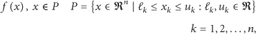
This algorithm is applied to the optimization problems with the limited variables as follows:

$$\begin{array}{r}\hfill f(x),x\in PP=\{x\in {\mathrm{\Re }}^n|{\mathrm{\ell }}_k\le x_k\le u_k;{\mathrm{\ell }}_l,u_k\in \mathrm{\Re }\}\\ \hfill k=1,2,\dots ,n,\end{array}$$

(1)

where n is the dimension of the solution space, $u_k$ is the upper limit of the solution space, ${\mathcal{l}}_k$ is the lower limit of the solution space, and $f\left(x\right)$ is function which will be minimized.

The metaheuristic EM algorithm consists of 4 procedures which are named initialize, local search, calculation, and movement.

The pseudocode of the metaheuristic EM algorithm is provided in Algorithm 1.

Algorithm 1: Electromagnetism-like algorithm.

 (1) Initialize

(2) iteration ← 1

(3) while iteration < maxiteration  do

(4) computing objective function value

(5) searcing local sample points

(6) calculating the charge and total force

(7) moving towards the total force

(8) iteration ← iteration + 1

(9) end while

Procedure 1: “Initialize.” In order to optimize a problem, some parameters must be set before it is benefiting from the EM algorithm. Most basic parameters are population size, the number of iterations, and dimension of the solution space. At the same time, the initializing of the population has been done in this procedure. Distribution of the m sample points is performed randomly in the solution space. Each coordinate of a point is assumed to be uniformly distributed between upper limit and lower limit of the solution space [23].

The pseudocode of the randomly generated population is provided in Algorithm 2.

Algorithm 2: Initializing population.

 (1) for   $$i=\mathit{1}$$ to m  do

(2)  for  k = 1 to n  do

(3)    λ←Uniform (0, 1)

(4)     $$x_k^i\leftarrow l_k+\mathrm{\lambda }\times (u_k-l_k)$$   

(5)  end for

(6) end for

Procedure 2: “Local Search.” This procedure is used to get related information for each sample point in the solution space. In this procedure, point y representing a new available point moves across the sample point x line with random step length between 0 and 1. If point y finds a more ideal point during the iterations, sample point x will be replaced with the new obtained point y. Thus, the best sample point is updated. In fact, local search is not necessary and can be ignored because it generally spends more time.

Procedure 3: “Charge and Total Force Calculation”. The total force on each particle is calculated according to Coulomb law. At the same time, the charge of every particle determines the attraction and repulsion forces of the particle. According to electromagnetism theory, the force applied to a particle by another particle is inversely proportional to the square of distance between these particles and is directly proportional with their own charges.

The charge of particle i, $q^i$ , is calculated by the following equation:

$$\begin{array}{r}\hfill q^i=exp\left\{-n\frac{f\left(x^i\right)-f\left(x^{\text{best}}\right)}{{\sum }_{j=1}^m[f(x^i)-f(x^{\text{best}})]}\right\},\\ \hfill i=1,2,\dots ,m,\end{array}$$

(2)

where n is the dimension of the solution space, m is the particle number, $f(x^i)$ is the objective function value of particle i, and $f(x^{\text{best}})$ is the best objective function value $(\arg \hspace{0.17em}\min \{f(x^i),\forall i\})$ among these particle values. The particle which has the best objective function value is named “optimum particle.” Because of the objective function value of this particle which has the smallest objective function value among the particles, the charged value of this particle will be 1 which is the maximum charge value.

The pseudocode of the calculating charges is provided in Algorithm 3.

Algorithm 3: Calculation of the charges of each particle.

 (1) for   $$j=\mathit{1}$$ to m  do

(2)    $${\displaystyle \sum }\left[f\left(x^j\right)-f\hspace{0.17em}\hspace{0.17em}\left(x^{\text{best}}\right)\right]\leftarrow \left(f\left(x^j\right)-f\hspace{0.17em}\hspace{0.17em}\left(x^{\text{best}}\right)\right)$$

(3) end for

(4) for  i = 1 to m  do

(5)    $$q^i$$ ← exp $$\left(-n\times \frac{\left(f\left(x^i\right)-f\hspace{0.17em}\hspace{0.17em}\left(x^{\text{best}}\right)\right)}{\sum \left[f\left(x^j\right)-f\hspace{0.17em}\hspace{0.17em}\left(x^{\text{best}}\right)\right]}\right)$$

(6) end for

After the calculation of the charge value of each particle in the solution space, the total force of the particle i, $F^i$ , is calculated with the help of the formula given as follows:

$$\begin{array}{cc}& F^i={\displaystyle \sum }_{j=\mathrm{1},j\ne i}^m\left\{\begin{array}{cc}\left(x^j-x^i\right)\frac{q^i{q}^j}{{‖x^j-x^i‖}^{\mathrm{2}}},\hfill & \text{if}\hspace{0.17em}\hspace{0.17em}f\left(x^j\right)<f\left(x^i\right)\hfill \\ \left(x^i-x^j\right)\frac{q^i{q}^j}{{‖x^j-x^i‖}^{\mathrm{2}}},\hfill & \text{if}\hspace{0.17em}\hspace{0.17em}f\left(x^j\right)\ge f\left(x^i\right).\hfill \end{array}\right.\end{array}$$

(3)

Calculated force $F^i$ is the total force of the forces which are applied to particle i and at the same time can be referred to as the resultant force. In (3), if $f(x^j)<f(x^i)$ , the attraction force is applied on particle $x^i$ by particle $x^j$ and the direction of the force is from $x^i$ to $x^j$ . If $f(x^j)\ge f(x^i)$ the repulsion force is applied on particle $x^i$ by particle $x^j$ and the direction of the force is from $x^j$ to $x^i$ .

The pseudocode of the calculating exerted total force is provided in Algorithm 4.

Algorithm 4: Calculation of the total force exerted to particles.

   (1) for   $$i=\mathit{1}$$ to m  do

  (2)  for   $$j=\mathit{1}$$ to m  do

  (3)    if   $$i\ne j$$   then

  (4)      if   $$f\left(x^j\right)<f\left(x^i\right)$$   then

  (5)        $$F^i\leftarrow F^i+\left(x^j-x^i\right)\times \left(\frac{q^i{q}^j}{{\Vert x^j-x^i\Vert }^{\mathit{2}}}\right)\left\{\text{Attraction}\right\}$$

  (6)     else

  (7)       $$F^i\leftarrow F^i-\left(x^j-x^i\right)\times \left(\frac{q^i{q}^j}{{\Vert x^j-x^i\Vert }^{\mathit{2}}}\right)\hspace{1em}\left\{\text{Repulsion}\right\}$$

  (8)     end if

  (9)    end if

(10)  end for

(11) end for

Thus, each particle in the solution space moves in the direction of the resultant force vector of attraction or repulsion forces applied to it as shown in Figure 2.

Figure 2

The sample of attraction or repulsion forces of the particles.

Procedure 4: “Movement towards the Total Force.” After the total force $F^i$ is calculated, particle i is moved to its new position which is obtained as

$$\begin{array}{r}\hfill x_k^i=\{\begin{array}{ll}{x}_k^i+\lambda \frac{F_k^i}{\Vert F^i\Vert }(u_k-x_k^i)\hfill & \text{if}\hspace{0.17em}{F}_k^i>0\hfill \\ x_k^i+\lambda \frac{F_k^i}{\Vert F^i\Vert }(x_k^i-l_k)\hfill & \text{otherwise}\hfill \end{array}\\ \hfill i=1,2,\dots ,m,\hspace{0.17em}\hspace{0.17em}\hspace{0.17em}k=1,2,\dots ,n,\hspace{0.17em}\hspace{0.17em}\hspace{0.17em}\hspace{0.17em}i\ne \text{best},\end{array}$$

(4)

where the random step length, λ, is assumed to be uniformly distributed between 0 and 1 $(0<\lambda \le 1)$ . According to (4), if $F^i>0$ the particle moves toward the upper bound; else the particle moves toward the lower bound. On the other hand, $x^{\text{best}}$ is the optimum particle, and thus it attracts the other particles and hence its location does not change.

The new location of the particle i is determined on condition that it moves between defined upper and lower bounds of the solution space by using (1).

The pseudocode of the calculating movement of each point is provided in Algorithm 5.

Algorithm 5: Calculation of the new position of particles.

   (1) for   $$i=\mathit{1}$$ to m  do

  (2)  if   $$i\ne best$$   then

  (3)     λ ←Uniform (0, 1)

  (4)    for   $$k=\mathit{1}$$ to n  do

  (5)     if   $$F_k^i>\mathit{0}$$   then

  (6)       $$x_k^i\leftarrow x_k^i+\mathrm{\lambda }\times \left(\frac{F_k^i}{\Vert F^i\Vert }\right)\left(u_k-x_k^i\right)$$

  (7)     else

  (8)       $$x_k^i\leftarrow x_k^i+\mathrm{\lambda }\times \left(\frac{F_k^i}{\Vert F^i\Vert }\right)\left(x_k^i-l_k\right)$$

  (9)     end if

(10)    end for

 (11)  end if

(12) end for

3. Dynamic Deployment Problem in WSNs and Sensor Detection Model

Dynamic deployment of the sensors in the network is one of the most important issues which have effects on the WSNs performance. Improvement of the WSNs performances with the help of increasing the capacities of sensor detection is related to the dynamic determination of their locations within the area. The location changes of the sensors which are nondynamic in the network cause the problem of dynamic deployment. For this reason, optimizing the dynamic deployment of sensors effectively increases coverage area of the network and improves performance of the WSNs.

The initial deployments of the sensors are chosen randomly because the sensors do not have any information about the detection area and then the deployments of them which determine their next location is made dynamically. In detection area, every sensor knows its own location information and they share their information with their neighbor sensors. Sensors in this area can communicate with the neighbor sensors in the communication range and mobile sensors can change their location by using this information. However, stationary sensors cannot change their first locations in the solution space [25].

In order to find the effective coverage area of WSNs, two sensor detection models are used. These models are the binary detection model and the probabilistic detection model. In this study, we used the binary detection model. It is assumed that every sensor has the same detection range r and sensor i, $s^i$ , is positioned at pixel point $(x^i,y^i)$ in the solution space.

The binary detection model [26] is calculated as follows:

$$\begin{array}{cc}& c_{xy}\left(s^i\right)=\left\{\begin{array}{cc}\mathrm{1},\hfill & \text{if}\hspace{0.17em}\hspace{0.17em}d\left(s^i,P\right)\le r\hfill \\ \mathrm{0},\hfill & \text{if}\hspace{0.17em}\hspace{0.17em}d\left(s^i,P\right)>r,\hfill \end{array}\right.\end{array}$$

(5)

where $d\left(s^i,P\right)$ is the Euclidean distance between $s^i$ and P which is any pixel point in coordinates $(x,y)$ in the solution space. $c_{xy}(s^i)$ is the coverage binary value of any pixel point P by the sensor $s^i$ . It means that if $d(s^i,P)<r$ , the pixel point P is covered by sensor of $s^i$ .

4. Dynamic Deployment of WSN with EM Algorithm

In this study, EM algorithm was used to find a solution to the dynamic deployment problem of WSNs. The reason is that EM algorithm is used to maximize the coverage rate of the sensor network. While the sensor deployment algorithm based on EM is being applied to sensor networks, the following network scenarios are considered.

• (i)

Detection radius r of all the sensors is the same.

(ii)

All of the sensors have the ability to communicate with the others.

(iii)

Sensors are mobile.

4.1. Suggested Coverage Rate Calculation

A new model is suggested in the calculation of the coverage rate of the network. Until now, to find solutions to the dynamic deployment problem of the network with the help of various optimization algorithms, in order to calculate the total coverage rate of the network [21, 27, 28], (6) was used as

$$\begin{array}{cc}& \text{CR}=\frac{{\displaystyle \bigcup }{c}_i}{A},\hspace{1em}i\in S,\end{array}$$

(6)

where $c_i$ is the coverage value of sensor i, S is the set of sensors, and A is the total size of the area of interest. Thus, the total coverage rate of the network, CR, is calculated with the help of dividing combination of coverage of the each sensor in the solution space to total size of the area.

In our model, each intersection of horizontal and vertical grid lines in the solution space represents a pixel point P. Coverage map which shows the coverage area of each sensor in the solution space is formed by pixel point matrices. Related values of this matrix, 0 and 1, represent the coverage situation of each pixel point P. If the matrix value is 1, it means that pixel point is covered by the sensor; else it means that the pixel point is not covered. In Figure 3 [29], a graphical representation of coverage map which is generated by using the pixel points is shown.

Figure 3

Generating the coverage map using the grid intersections (pixel points).

In our recommended model, total area of the coverage map is calculated such that

$$\begin{array}{cc}& d_c=\mathrm{1}+L_x\times \mathrm{2},\hspace{1em}\hspace{1em}{d}_r=\mathrm{1}+L_y\times \mathrm{2},\hspace{1em}\hspace{1em}A=d_c\times d_r,\end{array}$$

(7)

where $d_c$ is the column number of matrices, $d_r$ is the row number of matrices, $L_x$ is the unit length of x coordinate in the solution space, $L_y$ is the unit length of y coordinate in the solution space, and A is the total number of pixel points which represents the total area of the coverage map.

In this study, dimension of the solution space equals 2 and upper $u_k$ and lower $l_k$ limit of the solution space coordinate values are (50,50) and $(-50,-50)$ , respectively. Total area of coverage map A can be found by applying these coordinate values to (7). When it is calculated that $L_x$ is 100 units and $L_y$ is 100 units according to the defined coordinate values using (7), it is calculated that $d_c$ value is 101 units and $d_r$ value is 101 units. At the same time, A which shows both the total area of the sensor network and the total number of the pixel points in the coverage map is calculated as 10201.

In this study, the binary detection model of mobile wireless sensor network was calculated by using

$$\begin{array}{cc}& c_{xy}\left(P\right)=\left\{\begin{array}{cc}\mathrm{1},\hfill & \text{if}\hspace{0.17em}\hspace{0.17em}d\left(s^i,P\right)\le r,\hspace{1em}d\left(s^i,s^j\right)\le com\_r\hfill \\ \mathrm{0},\hfill & \text{otherwise},\hfill \end{array}\right.\end{array}$$

(8)

where $c_{xy}\left(P\right)$ is the binary value which shows the coverage of each pixel point P by sensors within the area of interest and $com\_r$ is a communication range which defines communication between the sensors. If the Euclidean distance between each pixel point P in the $(x,y)$ coordinate of the solution space and sensor $s^i$ is smaller than the detection radius of sensor r, pixel point P may uncover by the sensor $s^i$ . At the same time, it is controlled whether the sensor $s^i$ which covers the pixel point P is the neighbor with at least one sensor $s^j$ . Because, pixel point of P being covered only by the sensor $s^i$ is not an enough condition. If it is found that sensor $s^i$ is not a neighbor to any sensor $s^j$ in the communication range, there will be no communication between sensor $s^i$ and any other sensor in the sensor area and thus there will not be information to transmit. If the calculated binary value equals 1, the pixel point P is covered by the sensor $s^i$ . If this value equals 0, the pixel point P is uncovered by the sensor $s^i$ .

In our model, coverage rate (CR) was calculated by the equation

$$\begin{array}{cc}& \text{CR}=\frac{\sum c_{xy}\left(i\right)}{A},\hspace{1em}i\in S,\end{array}$$

(9)

where $\sum c_{xy}(i)$ is the total number of covered pixel points which has complied with the conditions in (8), S is the set of sensors, and A is the total area of the coverage map which is calculated by (7).

The pseudocode of the calculating of recommended coverage rate is provided in Algorithm 6.

Algorithm 6: Calculation of the recommended coverage rate.

    (1) $$k\leftarrow \mathit{1}\left\{k\in n\right\}$$ ,   $$covered\left(c_{xy}\right)\leftarrow \mathit{0}$$

   (2) for   $$y=l_{k+\mathit{1}}$$ to $$u_{k+\mathit{1}}$$   do

   (3)   for   $$x=l_k$$ to $$u_k$$   do

  (4)    $$P\leftarrow [x,y]$$

  (5)    for   $$i=\mathit{1}$$ to m  do

  (6)      for   $$j=\mathit{1}$$ to m  do

  (7)        if   $$i\ne j$$   then

  (8)         if   $$d(s^i,P)\le r$$   and   $$d(s^i,s^j)\le com\text{\_}r$$   then

  (9)            $$c_{xy}\left(P\right)\leftarrow \mathit{1}$$   {pixel point P is covered}

(10)            $$covered\left(c_{xy}\right)\leftarrow covered\left(c_{xy}\right)+\mathit{1}$$

 (11)         else

(12)            $$c_{xy}\left(P\right)\leftarrow \mathit{0}$$   {pixel point P is uncovered}

(13)         end if

(14)        end if

(15)      end for

(16)    end for

(17)   end for

(18) end for

(19) $$\text{CR}\leftarrow covered\left(c_{xy}\right)/A$$

4.2. Optimal Sensor Detection Algorithm Based on EM Algorithm

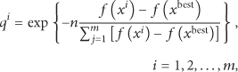
Based on EM algorithm, optimal sensor detection algorithm has been developed in order to carry out dynamic distribution of the sensors within the area more effectively. The aim of the algorithm is to determine whether any sensor is in optimal location by taking the updated locations of sensors within the area as base, after applying EM algorithm on the sensors with random initial distribution. In this phase, at first, the Euclidean distances of a sensor from the other sensors in the area are compared with the predefined distance parameters. These parameters are OPT_LOWERBOUND_DIST (optimal lower bound distance) and OPT_UPPERBOUND_DIST (optimal upper bound distance) which are the first conditions for any sensor to be optimal and which control the lower and upper bounds of the predefined optimal neighbouring distance and MAX_CONVERGENCE_DIST (maximum convergence distance) which is the second condition for being optimal and which controls the maximum convergence distance of only optimal sensors to any sensor. The number of neighbour sensors which are converge to each sensor in the area and become optimal is calculated grounding on these distance parameters predefined. The number of sensors which converge to any sensor by the distance defined via the OPT_LOWERBOUND_DIST and OPT_UPPERBOUND_DIST parameters is calculated defining with the OPT_NEIGHBOUR_COUNT (optimal neighbour sensors count) parameter. If there is any sensor that converges to a sensor has smaller than the distance defined with MAX_CONVERGENCE_DIST, this sensor will be non-optimal and the number of this sensor's non-optimal neighbour sensors are calculated by the NONOPT_NEIGHBOUR_COUNT parameter. The conditions for being optimal for any sensor can be considered in two cases: the number of calculated optimal neighbour sensors (OPT_NEIGHBOUR_COUNT) must be at least 1 and the number of calculated nonoptimal neighbour sensors (NONOPT_NEIGHBOUR_COUNT) must be equal to 0. The sensors in the area which comply with this condition are transferred to the OPT_SENSORS[ ] sequence and the number of sensors to the OPT_SENSORS_COUNT (optimal sensors count) parameter. In conclusion, sensors which are placed in optimal locations according to the distance parameters defined grounding on convergence conditions are calculated by this suggested algorithm. As it is demonstrated in Figure 4 [30], the desired state in the suggested sensor detection algorithm based on EM is to make sensors converge to each other so they will be optimal.

Figure 4

Optimal sensor distribution.

The pseudocode of the optimal sensor detection algorithm is provided in Algorithm 7.

Algorithm 7: Optimal sensor detection algorithm.

   (1) OPT_SENSORS_COUNT  ←  LENGTH( $$OPT\_SENSORS[]$$ )

  (2) for   $$i=\mathit{1}$$ to m  do

  (3) OPT_NEIGHBOUR_COUNT  ←  0, NONOPT_NEIGHBOUR_COUNT  ←  0

  (4)  if sensor of i is not include to OPT_ $$SENSORS[]$$   then

  (5)     for  j $$=\mathit{1}$$ to OPT_SENSORS_COUNT  do

  (6)       if   $$d\left(s^i,s^j\right)$$   between  OPT_LOWERBOUND_DIST  and  OPT_UPPERBOUND_DIST  then

  (7)         OPT_NEIGHBOUR_COUNT  ←  OPT_NEIGHBOUR_COUNT  + 1

  (8)       else if   $$d\left(s^i,s^j\right)<$$   MAX_CONVERGENCE_DIST

  (9)         NONOPT_NEIGHBOUR_COUNT  ←  NONOPT_NEIGHBOUR_COUNT + 1

(10)       end if

 (11)     end for

(12)     if (NONOPT_NEIGHBOUR_COUNT $$==\mathit{0}$$ AND OPT_NEIGHBOUR_COUNT   $$>=\mathit{1}$$ ) then

(13)        OPT_SENSORS_COUNT  ←  OPT_SENSORS_COUNT  + 1

(14)        OPT_SENSORS[OPT_SENSORS_COUNT]  ←  i

(15)     end if

(16)  end if

(17) end for

4.3. Applying the EM Algorithm for the Dynamic Deployment Problem

Applied algorithm steps in the solution of the dynamic deployment problem of WSNs are as shown in Algorithm 8.

Algorithm 8: The suggested EM algorithm based on sensor deployment algorithm.

   (1) Initialize

  First of all, the parameters which are used in the algorithm are described. These parameters are

  sensor detection radius r, communication range of the sensors $$com\_r$$ , the size of the coverage area

  A, the number of mobile sensors m, dimension of the population n, the maximum number of

  iteration $$maxitertation$$ , the maximum number of simulation $$maxrun$$ .

  (2) $$run=\mathit{1}$$

  (3) while    $$run<=maxrun$$

  (4) $$iter=\mathit{1}$$

  (5) Deploy the sensors randomly

  Deployment of the mobile sensors distribute in the solution space as given by Algorithm 2.

  (6) while    $$iter<=maxiteration$$

  (7) Calculate the objective function ( $$f_x$$ ) values of the sensors

  In order to calculate the charges of the sensors which are deployed in the solution space randomly

  according to the particle model in the EM algorithm, the objective function value of each sensor is

  calculated based on their existing positions as follows:

           $$f\left(x^i\right)={\displaystyle \sum }_{k=\mathit{1}}^n{x}_k^i\left(u_k-l_k\right)$$ ,  $$i=\mathit{1},\dots ,m$$ ,              (12)

  where $$f(x^i)$$ is the objective function value of sensor i,   $$x_k^i$$ is the coordinate value in the $$k\text{th}$$

  dimension of the sensor i.

  (8) Calculate charge of the sensors

  Sensors used in the network are assumed as a charged particle in the solution of the dynamic

  deployment problem. In order to calculate attraction-repulsion forces between the sensors based on

  the particle model of the EM algorithm which is expressed by Algorithm 1, the charge values of

  each sensor $$q^i$$ are calculated using (2).

  (9) Detect the optimal distributed sensors

  Sensors which have been placed in optimal locations are detected with the help of the optimal

  sensor detection algorithm stated in Algorithm 7, by using the distance parameters defined in

  Section 4.2.

(10) Calculate the resultant force of non-optimal sensors

  A resultant force, $$F^i$$ , which is calculated according to (3) by adding up the forces applied by

  the other sensors in the area to each sensor, is not optimal as a result of not being able to be placed

  in an optimal location, is applied to the non-optimal sensors. There is no need to calculate the

  resultant forces of optimal sensors. Because as it is stated on the next step, the 11th step, once the

  sensors are placed on optimal locations, their placements will not be changed so on.

 (11) Update the locations of non-optimal sensors

  Each non-optimal sensor in the area updates its current location according to Algorithm 5 by

  moving in the direction of the resultant force applied on it. The new position of non-optimal sensors

  is calculated using (4).

(12) $$iter=iter+\mathit{1}$$

(13) end while

(14) Find the coverages of grid points

  Coverage of every grid point by the sensors in the area being calculated using (8) which is

  expressed by Algorithm 6.

(15) Calculate the total coverage rate of sensor area, according to coverage map

  After the reaching predefined the maximum number of iterations, the total coverage rate of the

  WSNs is calculated using (9).

(16) $$run=run+\mathit{1}$$

(17) end while

Each solution space in this algorithm represents an array that has m elements. Table 1 shows the solution array. The positions ( $x,y$ ) of mobile sensors within the area are elements of the solution array.

Table 1

Solution array.

1	2	3	4	5	⋯	m
$$x_{\mathit{1}}$$	$$x_{\mathit{2}}$$	$$x_{\mathit{3}}$$	$$x_{\mathit{4}}$$	$$x_{\mathit{5}}$$	⋯	$$x_m$$
$$y_{\mathit{1}}$$	$$y_{\mathit{2}}$$	$$y_{\mathit{3}}$$	$$y_{\mathit{4}}$$	$$y_{\mathit{5}}$$	⋯	$$y_m$$

5. Results of the Simulation

In order to determine that the distribution algorithm based on EM which was suggested in this paper performs the dynamic distribution of mobile sensors more effectively, its performance has been compared with original ABC- and PSO-based distribution algorithms [31]. In this section, firstly parameters of the algorithms were selected based on PSO and ABC. Then, parameter selection of the suggested algorithm based on EM has been done under the experimental conditions and presented in detail as case studies.

5.1. Parameter Selection for PSO and ABC Algorithms

PSO's first version [32] has been applied in the dynamic distribution of sensors. Each particle is distributed randomly and the particles are updated in two phases. In the first phase, rate is measured as demonstrated in (10) as

$$\begin{array}{lll}{v}_{il}\hfill & =\hfill & v_{il}+c_1*\hspace{0.17em}\text{rand}\hspace{0.17em}()*(p_{il}-x_{il})\hfill \\ \hfill & \hfill & +c_2*\hspace{0.17em}\text{rand}\hspace{0.17em}()*(p_{gl}-x_{il}).\hfill \end{array}$$

(10)

In the second phase, locations of the particles in the area are updated using the $x_{il}=x_{il}+v_{il}$ . $\text{rand}()$ functions produce random numbers between (0,1). $p_{il}$ indicates the best location of the ith particle, $p_{gl}$ indicates the best location of the particles neighbouring the ith particle, $x_{il}$ indicates the location of the ith particle, and $v_{il}$ indicates its rate. $c_1$ and $c_2$ are the fixed positive parameters [16, 32, 33] that determine the performance of the algorithm and they are calculated by using (11) [31] as

$$\begin{array}{cc}& c_{\mathrm{1}}=\underset{c_{\mathrm{1}}}{\mathrm{Max}}-\left(\underset{c_{\mathrm{1}}}{\mathrm{Max}}-\underset{c_{\mathrm{1}}}{\mathrm{Min}}\right)*\frac{t}{t^{\max }},\\ c_{\mathrm{2}}=\underset{c_{\mathrm{2}}}{\mathrm{Max}}-\left(\underset{c_{\mathrm{2}}}{\mathrm{Max}}-\underset{c_{\mathrm{2}}}{\mathrm{Min}}\right)*\frac{t}{t^{\max }}.\end{array}$$

(11)

In (11), ${\mathrm{Max}}_{c_1}$ , ${\mathrm{Min}}_{c_1}$ , ${\mathrm{Max}}_{c_2}$ , and ${\mathrm{Min}}_{c_2}$ are the parameters that affect the performance of the algorithm. t indicates iteration time and $t^{\max }$ indicates maximum iteration time. As a result of the experiments carried out, the ${\mathrm{Min}}_{c_1}$ and ${\mathrm{Min}}_{c_2}$ parameters that provide the best performance for both PSO and ABC have been taken as 1, and the ${\mathrm{Max}}_{c_1}$ and ${\mathrm{Max}}_{c_2}$ parameters have been taken as 3.4 [31].

5.2. Parameter Selection for the Suggested Algorithm Based on EM

Case studies have been presented in this paper in order to determine the most suitable parameters to optimizing dynamic distribution of sensors by using the suggested distribution algorithm based on EM. In the case studies, 100 mobile sensors were distributed in a two-dimensional and 10,201 m² sensor area, and 10 Monte Carlo simulations were run, independently. r and $com\_r$ parameters have been taken as 7 meters and $2r$ (14 meters), respectively.

Two scenario were done for each case study, and the OPT_LOWERBOUND_DIST, OPT_UPPERBOUND_DIST and MAX_CONVERGENCE_DIST parameters have been taken as $\sqrt{3}r$ , $\sqrt{3.2}r$ , and $\sqrt{1}r$ in the 1st scenario and as $\sqrt{3}r$ , $\sqrt{3.5}r$ , and $\sqrt{1.3}r$ in the 2nd scenario, respectively. The OPT_NEIGHBOUR_COUNT parameter has been taken as 1 to be common for both the scenarios in the case studies except for the case study 3. As it is demonstrated in Figure 4, maximum distance between sensors must be $\sqrt{3}r$ in order to provide a perfect dynamic distribution [30]. Therefore, in order to carry out optimum dynamic distribution of the sensors in the area, the distance parameters in our case studies have been defined in the ranges indicated in the scenarios.

The simulations in this paper have been tested on a computer with 2.53 GHZ Core 2 Duo processor and 6.0 GB RAM, running with the MATLAB R2014a software.

5.2.1. Case Study 1: Sensors That Are in Optimal Locations according to Iteration Number

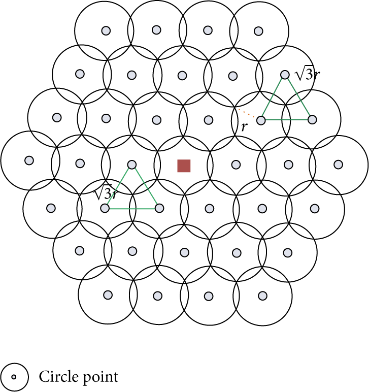
In this case study, the number of sensors that were placed in optimum locations has been calculated according to the iteration number by using the suggested distribution algorithm and the distance parameters defined in each scenario after the initial random distribution of the sensors in the area, and the results of the simulation are presented on Table 2.

Table 2

Simulation results of the optimal sensors count obtained along the iterations run for each scenario.

Scenarios	OPT_LOWERBOUND_DIST–OPT_UPPERBOUND_DIST	MAX_CONVERGENCE_DIST	The number of iterations	The average number of optimal sensors	Average running time (second)
Scenario 1	$$\sqrt{\mathit{3}}r\text{–}\sqrt{\mathit{3.2}}r$$   (12.1–12.5 meters)	$$\sqrt{\mathit{1}}r$$   (7 meters)	50	48	21.77
			100	69	37.46
			150	79	48.22
			200	87	49.08
Scenario 2	$$\sqrt{\mathit{3}}r$$ , $$\sqrt{\mathit{3.5}}r$$   (12.1–13.1 meters)	$$\sqrt{\mathit{1.3}}r$$   (7.98 meters)	50	78	14.63
			100	85	22.89
			150	90	28.51
			200	91	33.74

It is demonstrated on Table 2 that is a result of both scenarios, the average number of optimal sensors increased steadily as the iteration number increased. It has been determined that the average number of optimal sensors obtained in the 2nd scenario is better than the other. The reason is that while the optimal lower and upper bound parameters (12.1–12.5 meters) and the maximum convergence distance parameter value (7 meters) defined in the 1st scenario are increasing, the bigger number of sensors has been placed in optimal locations. However, increasing optimal lower and upper bound parameters would enable nonoptimal sensors to be optimal sensors. In the end, a bigger number of sensors’ being placed in optimal locations would be possible.

In this study, because of the parameters in the 2nd scenario which provide the best results for the number of sensors placed in optimal locations are used as base, while, on average, only 9 sensors were in optimal locations in the iterations distributed randomly at the initial phase; 91 sensors were placed to optimal locations in the dynamic distribution done with the suggested sensor distribution algorithm based on EM algorithm after 200 iterations. The progress graphic of the average numbers of sensors which were placed in optimal locations along iterations for both the two scenarios is demonstrated in Figure 5.

Figure 5

Average number of optimal sensors according to iteration number.

According to the scenarios defined in this study, when the running times of the simulations are compared, according to the results demonstrated in Table 2, a more optimal running time was obtained in scenario 2 than the other scenario, at the same number of iterations. In conclusion, scenario 2 in this case study has provided a better solution, both in terms of the number of sensors placed in optimal locations and the running time of the simulations.

5.2.2. Case Study 2: Average Coverage Ratios of the Area according to the Iteration Number

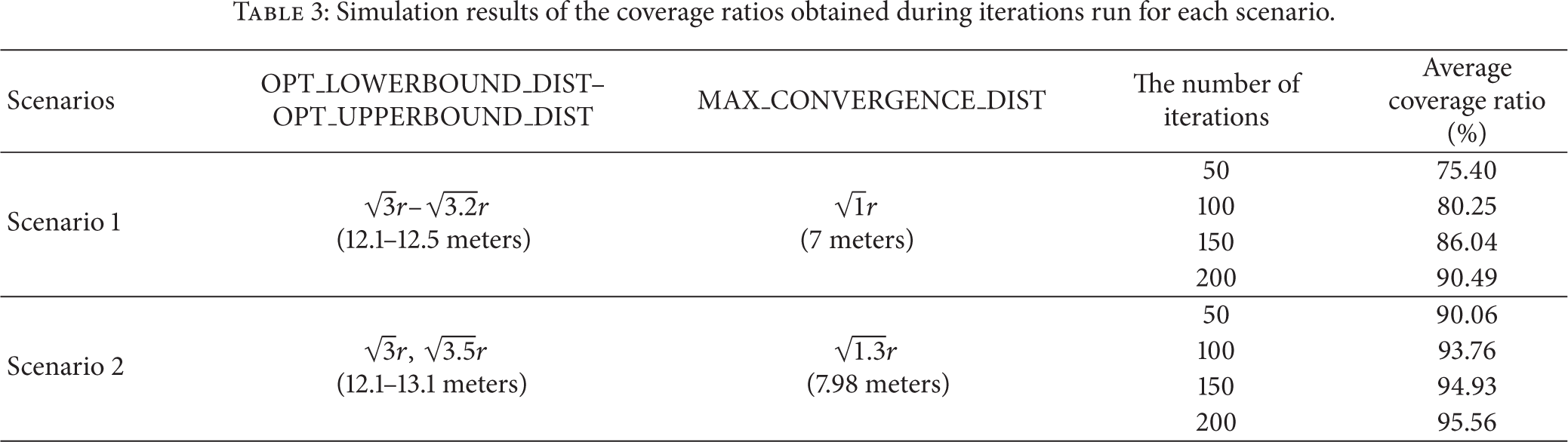
In this case study, it has been calculated that the average coverage ratios of the sensor area steadily increased as a result of running the distance parameters defined in both the scenarios during the iterations, and the results of the simulation are presented in Table 3. It has been determined that the coverage ratios obtained in scenario 2 are higher than the other scenario. First reason of this is that, as it is stressed in case study 1, the distance parameters chosen for scenario 2 enable a bigger number of sensors to be placed in optimal locations compared to the other scenario, and coverage ratios of the area in this scenario are bigger. Another reason for the coverage ratio to be higher is that, as a result of increasing the maximum convergence distance between the nonoptimal sensor and optimal sensors in scenario 2, the sensors that are to be optimal will be prevented to converge to each other anymore; thus the sensors that are in optimal locations would cover a larger area. In this case study, scenario 2 provided a better solution in terms of the ratio of sensor area's being covered.

Table 3

Simulation results of the coverage ratios obtained during iterations run for each scenario.

Scenarios	OPT_LOWERBOUND_DIST–OPT_UPPERBOUND_DIST	MAX_CONVERGENCE_DIST	The number of iterations	Average coverage ratio (%)
Scenario 1	$$\sqrt{\mathit{3}}r\text{–}\sqrt{\mathit{3.2}}r$$   (12.1–12.5 meters)	$$\sqrt{\mathit{1}}r$$   (7 meters)	50	75.40
			100	80.25
			150	86.04
			200	90.49
Scenario 2	$$\sqrt{\mathit{3}}r$$ , $$\sqrt{\mathit{3.5}}r$$   (12.1–13.1 meters)	$$\sqrt{\mathit{1.3}}r$$   (7.98 meters)	50	90.06
			100	93.76
			150	94.93
			200	95.56

While in Figure 6(a), initial locations of the sensors with %74.48 coverage ratio after random distribution are demonstrated, in Figure 6(b), optimal locations of the sensors with %95.56 optimal coverage ratio after 200 iterations following the application of the distance parameters in scenario 2 on the suggested sensor distribution algorithm are demonstrated.

Figure 6

Sensor distribution: (a) initial and (b) 200 iterations in scenario 2.

5.2.3. Case Study 3: Average Coverage Ratios of the Area according to Optimal Neighbour Count

Another one of the conditions defined in Algorithm 7 for every sensor in the area to be optimal is that a sensor should be a neighbour to at least one optimal sensor. In this case study, the effect of increasing the number of optimal neighbour sensors after 100 iterations in both scenarios on the number of optimal sensors reached in the area and on the coverage ratio of the area is calculated and results of the simulation are presented in Table 4.

Table 4

Simulation results according to optimal neighbour sensor count along the iterations run for each scenario.

Scenarios	OPT_LOWERBOUND_DIST–OPT_UPPERBOUND_DIST	MAX_CONVERGENCE_DIST	The number of optimal neighbour sensors (at least)	The average number of optimal sensors	Average coverage ratio (%)	Average running time (second)
Scenario 1	$$\sqrt{\mathit{3}}r\text{–}\sqrt{\mathit{3.2}}r$$   (12.1–12.5 meters)	$$\sqrt{\mathit{1}}r$$   (7 meters)	>=1	71	81.88	35.78
			>=2	6	64.39	47.34
			>=3	5	63.33	47.41
			>=4	3	63.01	47.43
Scenario 2	$$\sqrt{\mathit{3}}r$$ , $$\sqrt{\mathit{3.5}}r$$   (12.1–13.1 meters)	$$\sqrt{\mathit{1.3}}r$$   (7.98 meters)	>=1	85	92.15	23.39
			>=2	17	67.28	46.62
			>=3	7	63.08	47.21
			>=4	7	63.89	47.44

In this study, it has been detected in Table 4 that there were decreases in the number of sensors that were placed in optimal locations and average coverage ratio in both the scenarios, as optimal neighbour sensor count was increased. Since both the scenarios were run with a low iteration number, increasing the number of optimal neighbour sensors would make it hard for every sensor to be placed in optimal locations. As a result, since fewer sensors would be placed in optimal locations, coverage ratio of the area would be lower accordingly. In the case where the number of optimal neighbour sensors, defined with the OPT_NEIGHBOUR_COUNT parameter in both the scenarios, is increased, simulations have to be run with a higher iteration number for the sensor to be optimal.

In this case study, simulations of the iteration numbers that need to be used in order to place sensors in optimal locations without decreasing the coverage ratio of the area, in the case that the number of optimal neighbour sensors in both the scenarios is increased grounding on the distance parameters in scenario 2 in Table 4, were run and presented in Table 5. As the number of optimal neighbour sensors was increased, average iteration number that needed to be run in the simulation in order to get the desired number of optimal sensors increased as well steadily, which actually shows us the solution to the problem that occurred in Table 4. Therefore, as a solution to this problem, more iterations would need to be done in direct proportion, while the number of optimal neighbour sensors was increased. It can be interpreted from the simulation results in Table 5 that as the number of iterations was increased, averagely at the same levels the number of optimal sensors and the coverage ratios were obtained.

Table 5

Simulation results of the effect of the number of optimal neighbour sensors on average the number of iterations.

The number of optimal neighbour sensors	The average number of iterations	The number of optimal sensors	Average coverage ratio (%)	Average running time (second)
1	56	80	90.29	15.84
2	200	80	91.58	36.48
3	4000	80	92.83	435.68
4	5443	80	86.50	701.66

In conclusion, as it is demonstrated in Figure 7, since average coverage area at same ratios would be obtained with a fewer number of iterations compared to the others in the case that the number of optimal neighbour sensors is taken as 1 as the best solution in this case study, sensors would converge more rapidly, in less time.

Figure 7

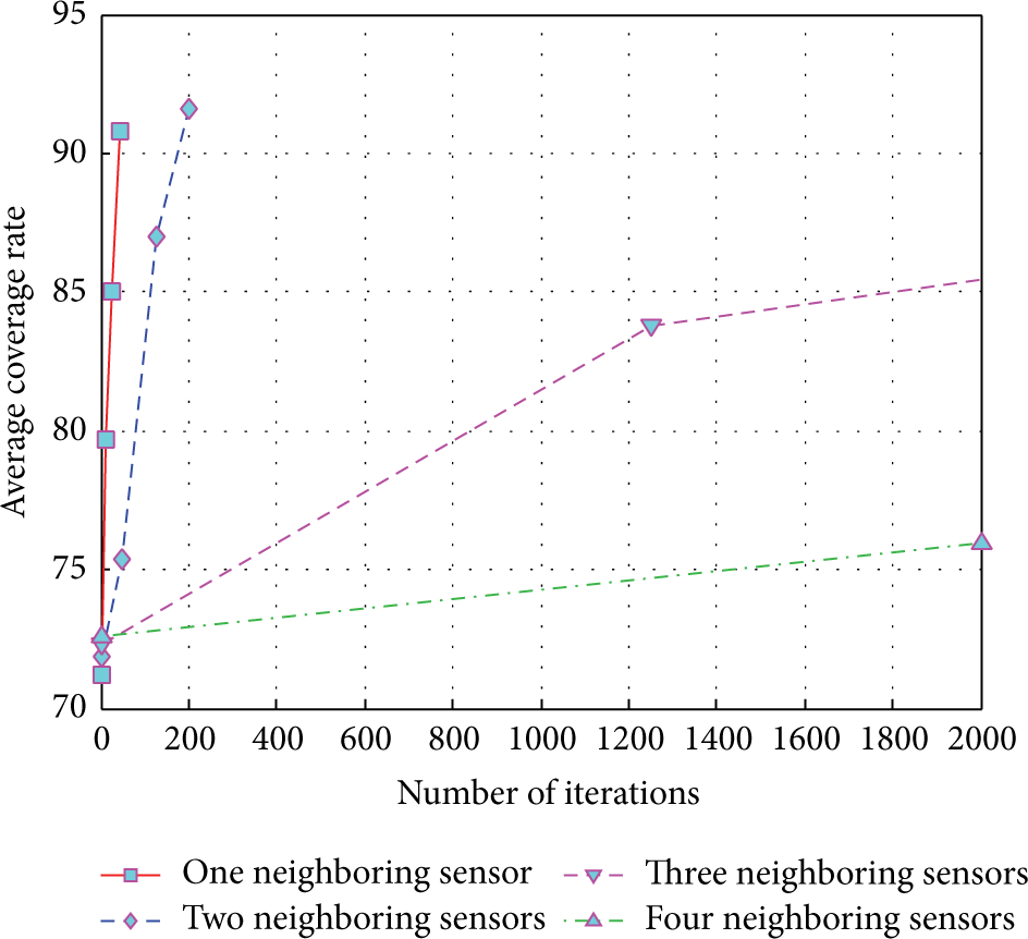
Progress of the coverage ratios of area during iterations, taking the number of optimal neighbour sensors as base.

5.2.4. Case Study 4: Optimal Energy Consumptions according to the Movement Distances of the Sensors

Improving energy efficiencies of sensors by minimising their energy consumptions is very important in terms of their lifetimes because sensors have only a limited amount of energy. Total movement distances of sensors are calculated by taking their initial random locations and target locations after their last iterations as base. The more location changes the sensors have in the area, the more energy they will consume. Also, since sensors’ changing fewer locations would optimise their power consumptions, it would enable their lifetimes to be longer as well.

In this case study, optimal energy consumption will be detected by comparing energy consumptions in both the scenarios via taking each sensor's total movement distance with the suggested distribution algorithm. 100 iterations were performed in 10 simulations in each of the two scenarios, according to the defined distance parameters in this study, and after each scenario, total movement distances of the sensors were calculated and their comparison are demonstrated in Figure 8. According to this comparison, average movement distance in Scenario 1 is 5518.9 meters, and in scenario 2, it is 4207.5. According to the results of the simulation, it has been detected that energy consumptions of the sensors dynamic distributions of which were done taking the distance parameters as base were optimal in scenario 2 as compared to those in scenario 1. Therefore, scenario 2 has offered a better solution than the other.

Figure 8

Progress of the total movement distances of all the sensors in the area.

5.3. Simulations in an Ideal Medium

100 mobile sensors with detection radius of 7 meters each were used in an ideal medium of 10,000 m² where there were no obstructions that would inhibit the distribution of sensors to the desired zone in the wireless area. In order to obtain more reliable results while comparing the suggested sensor distribution algorithm with the other algorithms, dynamic distribution of the sensors was done running 20 Monte Carlo simulations on condition that the values of the size of the area, the number of mobile sensors in the area, and detection radiuses of the sensors are the same. While performing distribution of the sensors with the suggested distribution algorithm based on EM, the parameters in scenario 2 which were applied in case studies in Section 5.2 and gave optimal results each time were used.

The first criterion in the algorithms compared in this paper is coverage ratios of sensor area. In each iterations, random distribution of the sensors was done independently and coverage ratios of the mentioned medium were calculated after 100, 500, 2000, 5000, and 10000 iterations. Dynamic distribution results of the original ABC and PSO algorithms [31] and the suggested distribution algorithm, which were compared after running sensors in the area with the stated iterations, are demonstrated in Table 6.

Table 6

Results of the coverage ratios of the algorithms compared at the stated iterations.

Compared algorithms	The number of iterations
	100	500	2000	5000	10000
EM	0.9553	0.9812	0.9907	0.9915	0.9960
Original ABC	0.9184	0.9713	0.9826	0.9848	0.9863
PSO	0.7993	0.8097	0.8403	0.9215	0.9431

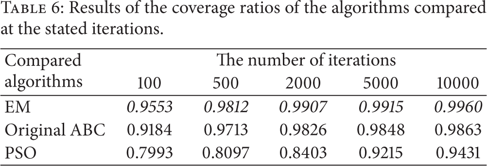
According to the iteration results demonstrated in Table 6, better coverage ratios were obtained in the suggested distribution algorithm compared to ABC and PSO coverage ratios. Moreover, after only 100 iterations, the suggested algorithm performed optimal distribution of the sensors in a short time and it means that the suggested algorithm converges the sensors more rapidly than the other two algorithms. The reason of this is that, once each sensor in the area, dynamic distribution of which is done according to Algorithm 8, is placed in an optimal location, its location does not change during the iterations again.

Optimal distribution of the sensors after running the suggested sensor distribution algorithm in this paper during the stated iterations is demonstrated in Figure 9. In these figures, pink nodes represent sensors, blue circles represent detection ranges of the sensors, and green areas represent the covered grid area. According to these figures, we can conclude that sensors covered the area effectively, doing a more rapid convergence with the use of the suggested sensor distribution algorithm, according to the numbers of iteration.

Figure 9

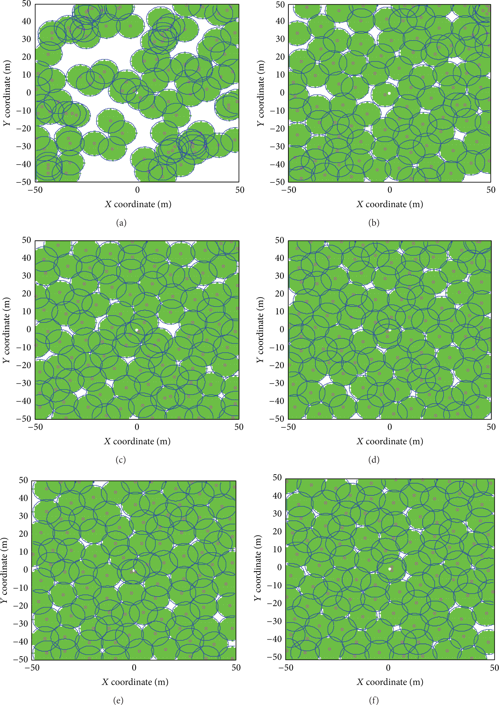
Sensor distribution: (a) initial, (b) 100 iterations, (c) 500 iterations, (d) 2000 iterations, (e) 5000 iterations, and (f) 10000 iterations.

Performances of EM-, original ABC-, and PSO-based sensor distribution algorithms are compared in Figure 10. In order to make this comparison more reliable, initial random distribution ratio of the suggested sensor distribution algorithm was taken lower than the initial random distribution ratios of the compared algorithms, determined as 74.75%, keeping the same initial random distribution ratios of the original ABC and PSO algorithms [31]. The reason for this is to show that, even though the initial random distribution ratio of the suggested distribution algorithm was lower, it provides a more rapid convergence compared to the other algorithms, reaching a higher coverage ratio which is 95.53% in 100 iterations as it is demonstrated in Table 6. In conclusion, we can say that, in this comparison, the suggested sensor distribution algorithm based on EM algorithm provides mobile sensors’ distribution in the area with a more rapid convergence and has better performance than ABC- and PSO-based distribution algorithms based on the achieved optimal coverage ratios.

Figure 10

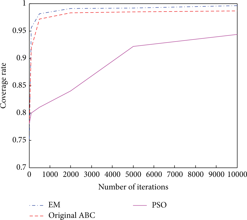
Progress of coverage ratios of the area during iterations in the simulations by the EM, original ABC and PSO algorithms.

Another criterion in the algorithms compared in this paper is total movement distances of sensors. As it is stated in case study 4 in Section 5.2.4, if the sensors’ total movement distances are low, their energy consumptions will be low and their lifetimes will be affected positively. As suggested in the comparisons, EM-based sensor distribution algorithm's average of the total movement distances in each iteration demonstrated in Table 6 is 4410.16 meters; the ABC's is 5216.1 meters [31], and because the worst coverage ratio was obtained in the PSO algorithm, its total movement distance was not compared. According to these results, we can say that, because the suggested EM-based sensor distribution algorithm's total movement distance is less, its energy consumption is better, compared to the original ABC algorithm.

6. Conclusion

Using binary detection model, an EM based sensor distribution algorithm consisting of only mobile sensors was suggested in this paper to optimise sensors in a wireless area. Simulation results have indicated that the suggested sensor distribution algorithm has better performance, giving better results than the original ABC- and PSO-based algorithms, when the criteria of comparison, which are coverage ratio of the area, convergence rate of sensors, and their total movement distances, are taken as the base. Our future study that we plan on doing in this area will be the application of the EM algorithm not only on mobile sensors but also on stationary sensors.