Sage Journals: Discover world-class research

Abstract

Wireless sensor networks have often been used to monitor environmental conditions, such as temperature, sound, and pressure. Because the sensors are expected to work on batteries for a long time without charging their batteries, the major challenge in the design of wireless sensor networks is to enhance the network lifetime. Recently, many researchers have studied the problem of constructing virtual backbones, which are backbones used for different time periods, to prolong the network lifetime. In this paper, we study the problem of constructing virtual backbones in dual-radio wireless sensor networks to maximize the network lifetime, called the Maximum Lifetime Backbone Scheduling for Dual-Radio Wireless Sensor Network problem, where each sensor is equipped with two radio interfaces. The problem is shown to be NP-complete here. In addition, rather than proposing a centralized algorithm, a distributed algorithm, called a Dominating-Set-Based Algorithm (DSBA), is proposed for a wide range of wireless sensor networks to find a backbone when a new one is required. Simulation results show that the proposed algorithm outperforms some existing algorithms.

1. Introduction

Wireless sensor networks are composed of many wireless sensors deployed in a wide range of areas, where each sensor is able to communicate with others through intersensor wireless communication [1–5]. The wireless sensor networks are able to collect, process, and store environmental information [6–8]. In wireless sensor networks, the batteries are the main energy sources of sensors, while the sensor nodes are expected to work in batteries for a long time without charging their batteries. Therefore, energy efficiency in wireless sensor networks is the main issue that we address in this paper.

Backbone is a well-known technique for various aspects of wireless sensor networks, such as routing, multicasting, and broadcasting [9, 10]. In the backbone technique, some nodes in the backbone always turn on their radio to maintain the activation of the network, and the rest of the nodes turn off their radio to save energy. Recently, many research studies are mostly designed to minimize the size of the backbone to, therefore, reduce the energy consumption in the network. In [11], an energy-efficient backbone construction algorithm is proposed for mobile ad hoc networks with adjustable transmission ranges. In [10], an algorithm was proposed to construct a backbone in the wireless sensor network such that the cost of routing would be reduced. In [12], Chuang and Chen proposed a novel heuristic-based backbone algorithm, called SmartBone. In SmartBone, two steps are required to form a backbone to improve energy saving in the network. The first step is to find backbone nodes by the proposed flow-bottleneck preprocessing method, and the second step is to reduce the number of redundant nodes by the proposed dynamic density cutback method. In [13], Zhang et al. proposed an algorithm to construct a connected backbone in the wireless sensor network such that the network achieves much higher throughput and delivery ratio and much lower end-to-end delay and routing distance.

Recently, some researchers focused on prolonging the network lifetime while using the backbone technique. The network lifetime is often determined by the time span from when the network is active to when one node in the backbone runs out of energy. In [14], Torkestani introduced an extended version of the connected dominating set problem for modeling the energy-efficient backbone formation problem in wireless sensor networks. In addition, an algorithm of constructing the network backbone was proposed to maximize the lifetime.

Because the nodes in the backbone are always active, their energy is depleted quickly so that the backbone is easily broken. Therefore, to prolong the network lifetime, some researchers studied scheduling nodes to become backbone nodes during some periods of time and nonbackbone nodes during other periods. In [15], Zhao et al. studied the problem of finding multiple backbones and scheduling the backbones to work for different time periods such that the network lifetime would be maximized. Hereafter, the multiple backbones used for different periods were called virtual backbones. The problem is shown to be NP-hard in [15]. In addition, centralized algorithms are proposed to find and schedule virtual backbones to maximize the network lifetime. However, centralized algorithms are often not feasible in a wide range of wireless sensor networks [16, 17].

In wireless sensor networks, sensors can be equipped with multiple radios to promote the capacity of wireless sensor networks, such as simultaneous data transmission and reception, and operations on different frequency bands. Several researchers study minimizing total energy consumption while using sensors having multiple radios [18–20]. In this paper, to maximize the network lifetime, we study the problem of scheduling virtual backbones for a dual-radio wireless sensor network such that the network lifetime is maximized. This Maximum Lifetime Backbone Scheduling for Dual-Radio Wireless Sensor Network problem occurs when each node in the network is equipped with two radio interfaces, including small-range radio and large-range radio. We first show that the problem is NP-complete, which implies that no polynomial time algorithm exists for the problem unless $P = N P$ . Rather than proposing a centralized algorithm of finding a list of backbones working sequentially to prolong the network lifetime, in this paper, we propose a distributed algorithm, termed Dominating-Set-Based Algorithm (DSBA), to find a backbone when a new backbone is required; that is, the network is initialized or one node in the backbone is going to run out of energy. The rest of this paper is organized as follows. Section 2 describes the details of the network model, introduces the Maximum Lifetime Backbone Scheduling for Dual-Radio Wireless Sensor Network problem, and shows its hardness. Section 3 proposes the DSBA. In Section 4, we provide the theoretical analysis to show the correctness of the DSBA. In Section 5, we evaluate the performance of the DSBA in terms of the network lifetime in wireless sensor networks. Finally, in Section 6, we conclude this paper.

2. System Model and Problem Definition

2.1. System Model

In dual-radio wireless sensor networks [21–23], each sensor is equipped with two radios whose ranges are r and R, respectively, where $r < R$ . Each sensor can use only one of the radios at the same time. When every sensor selects one radio for communication, two sensors can communicate with each other if any one of the sensors is within the radio range of the other sensor. The wireless sensor network can then be represented as an undirected weighted graph $G (V_{G}, E_{G}, w_{G})$ , where node $v \in V_{G}$ denotes a sensor in the networks, edge $(u, v) \in E_{G}$ represents the fact that u and v can communicate with each other, and $w_{G} (v)$ denotes the energy power of v for being backbone nodes. In the networks, the sink node is a special node that acts as a gateway between the networks and the outside networks. Here, the sink is assumed to have infinite energy power. Take Figure 1, for example, where the number near a node represents its corresponding energy, and node s is a sink. Figure 1(a) shows the wireless sensor network whose nodes use the same radio for communication. In addition, $w (f) = 9$ and $w (s) = \infty$ . Figure 1(b) shows the wireless sensor network in which nodes c, f, k, and s use large-range radios.

Figure 1

Example of dual-radio wireless sensor networks, where the number close to a node denotes the node's energy. (a) The network topology $G_{1} (V_{G_{1}}, E_{G_{1}}, w_{G_{1}})$ formed by the nodes using small-range radios. (b) The network topology $G_{2} (V_{G_{2}}, E_{G_{2}}, w_{G_{2}})$ formed by the nodes each using large-range or small-range radio.

Many applications in wireless sensor networks use backbone techniques to provide the benefits of routing, reducing signal interference, and energy saving [13, 15, 24]. A backbone is formed by some nodes in the networks and has the following two properties. The first is that the backbone is a connected subnetwork; that is, it is a connected subgraph $B (V_{B}, E_{B})$ in G, where $V_{B} \subseteq V_{G}$ and $E_{B} \subseteq E_{G}$ . The second is that any node in the networks is either a backbone node or a neighboring node of a backbone node; that is, for each $v \in V_{G}$ , $v \in V_{B}$ or edge $(u, v) \in E_{G}$ for some $u \in V_{B}$ . Here, we assume that if a node $v \in V_{G}$ has energy power greater than zero, v is able to be a backbone node; otherwise, it is a nonbackbone node and can use only a small-range radio to connect to the backbone. Take Figure 1, for example. $B_{1} (V_{B_{1}}, E_{B_{1}})$ and $B_{2} (V_{B_{2}}, E_{B_{2}})$ are backbones in Figures 1(a) and 1(b), respectively, where $V_{B_{1}} = {a, d, e, s}$ , $V_{B_{2}} = {b, c, f, k, s}$ , $E_{B_{1}} = {(a, s), (a, d), (a, e), (d, e)}$ , and $E_{B_{2}} = {(b, s), (b, c), (c, f), (k, s)}$ .

To reduce the energy consumption of sensors, we assume that each sensor in the networks is duty-cycled and has the same working cycle [15, 25, 26]. That is, the state of each sensor in the same working cycle is either in an active or sleep mode. If a sensor is in an active mode, the sensor turns on the radio for forwarding or receiving messages; otherwise, it turns off the radio to save energy. For simplicity, a working cycle is assumed to be one unit of time. To prolong the lifetime of wireless sensor networks, sensors are selected in turn to become backbone nodes for a number of working cycles. The backbones working in different periods of time are also called virtual backbones hereafter [9, 15]. When a virtual backbone is determined to work for some period of time, the nodes in the backbone are in an active mode, and the others are in a sleep mode in the period. Take Figure 1, for example. Let $B_{1} (V_{B_{1}}, E_{B_{1}})$ in Figure 1(a) be the virtual backbone of the wireless sensor network starting at time $0$ ; and the working time for $B_{1}$ is $2$ , where $V_{B_{1}} = {a, d, e, s}$ . Let $B_{2} (V_{B_{2}}, E_{B_{2}})$ in Figure 1(b) be another virtual backbone of the wireless sensor network starting at time $2$ ; and the working time for $B_{2}$ is $2$ , where $V_{B_{2}} = {b, c, f, k, s}$ . Note that nodes a, d, e, and s are active from time $0$ to time $2$ , and nodes b, c, f, k, and s are active from time $2$ to time $4$ . Also note that nodes c, f, and k use large-range radios from time $2$ to time $4$ .

In the networks, each node v is associated with an energy power $w_{G} (v)$ [27, 28]. For simplicity, we assume that $R = 2 r$ and a sensor with a small-range radio (or a large-range radio) in the backbone consumes $1$ (or $2$ ) unit of energy power for one unit of time. Therefore, the maximum time period for v with a small-range radio (or a large-range radio) to be a backbone node is $w_{G} (v)$ (or $⌊ w_{G} (v) / 2 ⌋$ ). Let the maximum lifetime of a sensor v, denoted by $l (v)$ , be the time span from when v is active to when its energy is depleted [15]. Take Figure 1, for example. Node a with a small-range radio in Figure 1(a) has maximum lifetime $l (a) = 2$ . In addition, node k with a large-range radio in Figure 1(b) has maximum lifetime $l (k) = 4 / 2 = 2$ . Let $V_{B} = {v_{1}, v_{2}, \dots, v_{k}}$ be the set of nodes in virtual backbone B. The maximum lifetime of backbone B, denoted by $l (B)$ , is defined as the time span from when the backbone is active to when the energy power of one node in B is depleted. That is, $l (B) = m i n (l (v_{1}), l (v_{2}), \dots, l (v_{k}))$ . Take Figure 1, for example. Let $B_{1} (V_{B_{1}}, E_{B_{1}})$ in Figure 1(a) be the virtual backbone of the wireless sensor network starting at time $0$ , where $V_{B_{1}} = {a, d, e, s}$ . Because $l (a) = 2$ , $l (d) = 2$ , and $l (e) = 2$ , we have $l (B_{1}) = 2$ . Therefore, backbone $B_{1}$ can work for, at most, two units of time. Note that after time $2$ , nodes a, d, and e have zero energy power and cannot become backbone nodes anymore. Later, suppose that another virtual backbone $B_{2}$ starts to work at time $2$ , where $V_{B_{2}} = {b, c, f, k, s}$ . Because $l (b) = 2 / 1 = 2$ , $l (c) = ⌊ 5 / 2 ⌋ = 2$ , $l (f) = ⌊ 9 / 2 ⌋ = 4$ , and $l (k) = 4 / 2 = 2$ , we have $l (B_{2}) = 2$ . Therefore, the backbone $B_{2}$ can continue to work for, at most, $2$ units of time. In a wireless sensor network, if virtual backbones $B_{1}, B_{2}, \dots, B_{p}$ work in turn for time periods $T_{1}, T_{2}, \dots, T_{p}$ , in which $T_{1} \leq l (B_{1}), T_{2} \leq l (B_{2}), \dots, T_{p} \leq l (B_{p})$ , the network lifetime is defined as the sum of the working time of the virtual backbones; that is, $\sum_{i = 1}^{p} T_{i}$ . In the previous example, the network lifetime is $2 + 2 = 4$ when virtual backbones $B_{1}$ and $B_{2}$ work in turn for time periods $2$ and $2$ , respectively.

When the wireless sensor network is initialized, we assume that each sensor can then periodically use small-range and large-range radios to associate with other sensors. Therefore, each node can have the information of nodes within its radio range r (or R), including the identification (ID) and residual energy power. Hereafter, the set of nodes within u's radio range r (or R) is denoted by $u \cdot N_{r}$ (or $u \cdot N_{R}$ ). Take Figure 1, for example. Because nodes b, d, k, and s are within a's radio range r, $a \cdot N_{r} = {b, d, k, s}$ . In addition, because nodes a, b, c, d, e, and k are within s's radio range R, $s \cdot N_{R} = {a, b, c, d, e, k}$ .

2.2. Problem Definition and Its Hardness

When we are given a dual-radio wireless sensor network, our problem is to find a schedule of virtual backbones, that is, a set of 2-tuples ${(B_{1}, T_{1}), (B_{2}, T_{2}), \dots, (B_{p}, T_{p})}$ , such that the network lifetime is maximized. Our problem, called the Maximum Lifetime Backbone Scheduling for Dual-Radio Wireless Sensor Network problem, is illustrated as follows:

INSTANCE: the dual-radio wireless sensor network;

QUESTION: does there exist a schedule of virtual backbones in the network, that is, a set of 2-tuples ${(B_{1}, T_{1}), (B_{2}, T_{2}), \dots, (B_{p}, T_{p})}$ , such that the network lifetime is not less than k?

In this paper, the Maximum Lifetime Backbone Scheduling problem [15] is used to show the hardness of the Maximum Lifetime Backbone Scheduling for Dual-Radio Wireless Sensor Network problem, as shown in Theorem 1. The Maximum Lifetime Backbone Scheduling problem is illustrated as follows:

INSTANCE: the single-radio wireless sensor network;

Theorem 1.

The Maximum Lifetime Backbone Scheduling for Dual-Radio Wireless Sensor Networks problem is NP-complete.

Proof.

The Maximum Lifetime Backbone Scheduling for Dual-Radio Wireless Sensor Networks problem clearly belongs to the NP class. In addition, because the Maximum Lifetime Backbone Scheduling problem [15] is NP-hard and is clearly to be the subproblem of the Maximum Lifetime Backbone Scheduling for Dual-Radio Wireless Sensor Networks problem, the proof is therefore completed.

3. The Dominating-Set-Based Algorithm (DSBA)

Because the Maximum Lifetime Backbone Scheduling for Dual-Radio Wireless Sensor Networks problem is NP-complete, it is hard to find an exact solution in polynomial time. Rather than finding a list of backbones working for different periods of time, our idea is to find a backbone for any given dual-radio wireless sensor networks when a new backbone is required for the networks. That is, when the network is initialized or one node in the backbone is going to run out of energy, we will find another new backbone for sustaining the network lifetime. For the problem, we propose a distributed algorithm, called a Dominating-Set-Based Algorithm (DSBA), to find a backbone for any given dual-radio wireless sensor network, where each backbone node has an energy power greater than zero. The DSBA contains three steps. In the first step, the DSBA finds a dominating set in the wireless sensor network such that the nodes in the set have much energy power, which is illustrated in Section 3.1. Here, a dominating set for a graph $G^{'} (V_{G^{'}}, E_{G^{'}})$ is a set $D \subseteq V_{G^{'}}$ such that each node $v \in V_{G^{'}}$ is either in D or is connected to one node $u \in D$ in $G^{'}$ [29, 30]. In the second step, a backbone is established based on the selected dominating set, which is described in Section 3.2. Finally, some redundant nodes are pruned from the backbone to reduce the size of the backbone and minimize total energy consumption, which is given in Section 3.3. The necessary notation used in the section is defined in Definition 2.

Definition 2.

Given a set of nodes S in a dual-radio wireless sensor network, node $v \in S$ is said to be the most powerful node in S if ( $w (v) > w (p)$ ) or ( $w (v) = w (p)$ and $v \cdot I D < p \cdot I D$ ) for all $p \in S - {v}$ , where $v \cdot I D$ denotes v's ID.

3.1. Construction of Dominating Set

In this step, our goal is to construct a dominating set for a given dual-radio wireless sensor network such that the nodes in the set have enough energy power to be the backbone nodes and can dominate all nodes in the network. Although the dominating set problem has been studied by many researchers [29, 31, 32], they do not consider the energy power while selecting nodes to be included in the dominating set. Therefore, in the subsection, we propose a distributed algorithm to construct the dominating set D for the network, called the distributed dominating set algorithm (DDSA), such that the nodes in D have enough energy to be the backbone nodes.

Let the nodes included in the dominating set be called dominating nodes. In the DDSA, our idea is to let the sink node be a dominating node first because the sink node is a powerful node. Then, if a node v has no energy power or has a dominating node within v's radio range r, v is not considered to be the dominating node; otherwise, v is considered to be a dominating node. Algorithm 1 shows the DDSA executed by every node in the network.

Algorithm 1: $DDSA (v)$ .

(1) if v is a white node and receives a message m that is a $B L A C K_S E T$ or $G R A Y_S E T$ message then

(2) if $w (v) = 0$ or m is a $B L A C K_S E T$ message then

(3) v is marked as gray.

(4) v uses a small-range radio to locally broadcast the $G R A Y_S E T$ message.

(5) else if m is a $G R A Y_S E T$ message from node u then

(6) if v is the most powerful node in $u \cdot N_{r}^{h} \cap v \cdot N_{r}^{h} \cup {v}$ then

(7) v is marked as black.

(8) v uses a small-range radio to locally broadcast the $B L A C K_S E T$ message.

(9) end if

(10) end if

(11) end if

Initially, every node v is marked as white. The sink node s is then marked as black and uses a small-range radio to locally broadcast the $B L A C K_S E T$ message. If a white node v receives the $B L A C K_S E T$ message, v marks itself as gray and uses a small-range radio to locally broadcast the $G R A Y_S E T$ message, including $v \cdot N_{r}^{h}$ , where $v \cdot N_{r}^{h}$ denotes the set of white nodes within v's small radio range r, as described in Lines 2–4 in Algorithm 1. Otherwise, if a white node v receives a $G R A Y_S E T$ or $B L A C K_S E T$ message but has no energy power for being backbone nodes, that is, $w (v) = 0$ , v marks itself as gray and locally broadcasts the $G R A Y_S E T$ message as described in Lines 2–4 in Algorithm 1. Otherwise, if a white node v receives a $G R A Y_S E T$ message from node u, and v is the most powerful node in $u \cdot N_{r}^{h} \cap v \cdot N_{r}^{h} \cup {v}$ , v marks itself as black and uses a small-range radio to locally broadcast the $B L A C K_S E T$ message, as described in Lines 5–9 in Algorithm 1. Note that if the $B L A C K_S E T$ (or $G R A Y_S E T$ ) message from node u is received by a node v, v updates its local information to set u as black (or gray).

Take Figure 1(b), for example. Initially, every node in the network is white. The sink node s first marks itself as black and locally broadcasts a $B L A C K_S E T$ message by using a small-range radio. Each of nodes a and b that receives the message will become gray and locally broadcasts a $G R A Y_S E T$ message as described in Lines 2–4 in Algorithm 1. Then nodes c and k that receive the $G R A Y_S E T$ message will become black because they have higher energy power, according to Lines 5–9 in Algorithm 1. In addition, nodes d and e become gray and locally broadcast $G R A Y_S E T$ messages because they have no energy power for being backbone nodes. Node f then becomes black because $w (f) > w (i) > w (h) > w (g)$ . In addition, node j becomes gray because node c is black. Finally, the DDSA constructs the set ${c, f, s, k}$ as the dominating set.

3.2. Establishment of Backbone

In this subsection, we propose a distributed backbone algorithm (DBA) to establish a backbone according to the dominating set constructed by the DDSA. In the DBA, the idea is first to treat the sink node as the smallest connected subnetwork having only one node. Then, the subnetwork gradually merges its nearby black nodes and suitable gray nodes that are obtained by the DDSA to form a larger connected subnetwork until a backbone of the network is established. After applying the DBA, the nodes in the network are either backbone nodes represented by the blue nodes or nonbackbone nodes represented by the yellow nodes and gray nodes. Algorithm 2 shows the DBA executed by every node in the network.

Algorithm 2: $DBA (v)$ .

$(1$ ) if v receives a $B A C K B O N E_R E Q_r$ (or $B A C K B O N E_R E Q_R$ ) message then

(2) v is marked as blue and uses a large-range radio to locally broadcast the $D B A_S E T_B$ message.

(3) v uses a small-range (or a large-range) radio in the backbone.

(4) else if v receives a message m from node u that is a $D B A_S E T_B$ or $D B A_S E T_Y$ message then

(5) v marks u as blue (or yellow) in its local information if m is a $D B A_S E T_B$ (or $D B A_S E T_Y$ ) message.

(6) if v is a gray node, $w (v) > 0$ , and there exists a blue node $p \in v \cdot N_{r}$ then

(7) v uses a large-range radio to locally broadcast the $D B A_S E T_Y$ message.

(8) v is marked as yellow and uses a small-range radio in the network.

(9) else if v is a black node then

(10) v is marked as blue and uses a large-range radio to locally broadcast the $D B A_S E T_B$ message.

(11) if there exists a blue node $p \in v \cdot N_{r}$ then

(12) v uses a small-range radio in the backbone.

(13) else if there exists a most powerful node $p \in Y_{r}$ , where $Y_{r}$ is the set of yellow nodes in $v \cdot N_{r}$ then

(14) v uses a small-range radio in the backbone and sends a $B A C K B O N E_R E Q_r$ message to p.

(15) else if there exists a most powerful node $p \in B_{R}$ , where $B_{R}$ is the set of blue nodes in $v \cdot N_{R}$ then

(16) v uses a large-range radio in the backbone and sends a $B A C K B O N E_R E Q_R$ message to p.

(17) else if there exists a most powerful node $p \in Y_{R}$ , where $Y_{R}$ is the set of yellow nodes in $v \cdot N_{R}$ then

(18) v uses a large-range radio in the backbone and sends a $B A C K B O N E_R E Q_R$ message to p.

(19) end if

(20) end if

(21) end if

In the DBA, every node is initially a black or gray node after applying the DDSA. The sink node s is then marked as blue and uses a large-range radio to locally broadcast the $D B A_S E T_B$ message that is used to inform other nodes about the existence of the blue node and the connected subnetwork. If a gray node v having enough power receives the message, v marks itself as yellow, which is used to denote v as the node close to the connected subnetwork and able to be a candidate for becoming a backbone node, which is described in Lines 6–8 of Algorithm 2. Node v also uses a large-range radio to locally broadcast the $D B A_S E T_Y$ message that is used to inform other nodes about the existence of the yellow node. Then v uses a small-range radio in the network later. If a black node v receives the $D B A_S E T_B$ or $D B A_S E T_Y$ message, it implies that v is close to the connected subnetwork. Node v then marks itself as blue and tries to find a yellow or blue node p such that v can connect to the connected subnetwork through p, which is described in Lines 9–20 of Algorithm 2. If v finds that there exists a blue node p in $v \cdot N_{r}$ , v can use a small-range radio to connect to the connected subnetwork by p. Otherwise, if v finds that there exists a most powerful yellow node p in $v \cdot N_{r}$ , v will send a $B A C K B O N E_R E Q_r$ message to request p to become a blue node and use a small-range radio in the backbone. Otherwise, if v finds that there exists a most powerful blue node in $v \cdot N_{R}$ , v will send a $B A C K B O N E_R E Q_R$ message to request p to use a large-range radio in the backbone. Otherwise, if v finds that there exists a most powerful yellow node in $v \cdot N_{R}$ , v will send a $B A C K B O N E_R E Q_R$ message to request p to become a blue node and use a large-range radio in the backbone.

Take Figure 1(b), for example. Assume that after applying the DDSA, the nodes c, f, s, and k are black nodes, and the others are gray nodes. In the DBA, the sink node s first marks itself as blue and locally broadcasts a $D B A_S E T_B$ message. Then, the nodes that are within s's large-radio range, that is, nodes a, b, c, d, e, and k, receive the $D B A_S E T_B$ message from s. Nodes a, d, and e are still gray nodes because their energy power is equal to zero. In addition, node b becomes yellow because blue node $s \in b \cdot N_{r}$ . Node c (or k) becomes blue because c (or k) is a black node. Because b is a most powerful yellow node in $c \cdot N_{r}$ , c requests b to become a blue node later. Then, b and c use a small-range radio in the backbone. Because blue node $s \in k \cdot N_{R}$ , k requests s to use a large-range radio in the backbone. Therefore, k and s use a large-range radio in the backbone. Later, when node f receives a $D B A_S E T_B$ or $D B A_S E T_Y$ message, f becomes a blue node that uses a large-range radio because f is a black node, and blue node $c \in b \cdot N_{R}$ . Node f then requests c to use a large-range radio in the backbone. When node g, h, i, or j receives a $D B A_S E T_B$ or $D B A_S E T_Y$ message, it becomes yellow because there exists a blue node in its small-range radio. After applying the DBA, b, c, k, f, and s are backbone nodes, where b uses a small-range radio, and the others use a large-range radio in the backbone.

3.3. Refinement of Backbone

When the DBA is completed, the nodes in the network are classified into backbone and nonbackbone nodes, where the blue nodes are backbone nodes, and the gray nodes and yellow nodes are nonbackbone nodes. In the next step, we provide a refinement for the generated backbone to minimize the size of the generated backbone or reduce the energy consumption of backbone nodes, where the refinement contains two rules mentioned in the following paragraph.

From the observation of the generated backbones, we discover that if a backbone node v can change its large-range radio to a small-range radio such that the backbone is still connected, the energy consumption of v for being a backbone node is reduced. Take Figure 2, for example. In Figure 2(a), backbone nodes u, v, x, and y use a large-range radio, but the distance between u and v is smaller than the radio range r. If we can change v's large-range radio to a small-range radio, as shown in Figure 2(b), the backbone is still connected, and the energy consumption of v for being a backbone node is, thus, reduced. Therefore, the first rule is to change one backbone node's radio in such case, as described in Rule 1.

Figure 2

An example of reducing the energy consumption of backbone nodes. (a) Nodes u, v, x, and y use a large-range radio in the backbone. (b) Node v uses a small-range radio, and the others use a large-range radio in the backbone.

Rule 1.

Given a backbone B, let v be any node that uses a large-range radio in B. Assume that $G^{'} = (V_{G^{'}}, E_{G^{'}})$ is formed by v and all its neighboring nodes in the backbone, where $V_{G^{'}} = {u_{1}, u_{2}, \dots, u_{k - 1}, v}$ . If $G^{'}$ is a k-clique network, there exists a node $p \in V_{G^{'}}$ , $p \in v \cdot N_{r}$ , and p is the most powerful node in ${v, p}$ ; v can change to a small-range radio in the backbone.

To minimize the size of the generated backbone, some nodes can be pruned from the backbone if they are redundant. That is, if all the neighboring nodes of a backbone node v having a small-range radio in the backbone are dominated by another backbone node u, v is considered as a redundant backbone node and can be pruned. Take Figure 3, for example. In Figure 3(a), nodes u and v are backbone nodes. It shows that the set of the neighboring nodes of a backbone node u is ${v, x, y, z}$ , and the set of the neighboring nodes of a backbone node v is ${u, x, y}$ . Clearly, all neighboring nodes of node v in the backbone, that is, nodes u, x, and y, can be dominated by node u. Therefore, v can be pruned from the backbone, which is shown in Figure 3(b). Therefore, the second rule is to reduce the number of redundant backbone nodes in such case, as described in Rule 2.

Figure 3

An example of pruning redundant backbone nodes. (a) The network has a redundant backbone node v. (b) Node v is pruned from the backbone, shown in (a).

Rule 2.

Given a backbone B, let v be any node that uses a small-range radio in B. Node v can be pruned from the backbone if there exists another backbone node u such that $u \in v \cdot N_{r}$ , $v \cdot N_{r} - {u} \subseteq u \cdot N_{r} - {v}$ , and u is the most powerful node in ${u, v}$ .

4. Analysis of the DSBA

Assume that the dual-radio wireless sensor network is connected when every sensor uses a small-range radio. Also assume that every sensor has energy power greater than zero. Theorem 6 shows that the DSBA constructs a backbone for the network by Lemmas 3–5.

Lemma 3.

In the DDSA, the set of the black nodes in the dual-radio wireless sensor network forms a dominating set.

Proof.

Here, we first show that (S1) any white node v in the network that receives a $G R A Y_S E T$ message from node u will become a gray or black node later in the DDSA. Clearly, v will become a black node if v is the most powerful node in $u \cdot N_{r}^{h} \cap v \cdot N_{r}^{h} \cup {v}$ . It suffices to show that v will become a gray or black node if v is not the most powerful node in $u \cdot N_{r}^{h} \cap v \cdot N_{r}^{h} \cup {v}$ . Let $p_{1}^{1}, p_{2}^{1}, \dots, p_{n}^{1} \in u \cdot N_{r}^{h} \cap v \cdot N_{r}^{h} \cup {v}$ be more powerful than v, and $w (p_{1}^{1}) > w (p_{2}^{1}) > \dots > w (p_{n}^{1}) > w (v)$ . If $p_{1}^{1}$ does not become a black node later, it implies that there exists a white node $p_{1}^{2} \in u \cdot N_{r}^{h} \cap p_{1}^{1} \cdot N_{r}^{h} \cup {p_{1}^{1}}$ more powerful than $p_{1}^{1}$ . If $p_{1}^{2}$ does not become a black node later, it implies that there exists a white node $p_{1}^{3} \in u \cdot N_{r}^{h} \cap p_{1}^{2} \cdot N_{r}^{h} \cup {p_{1}^{2}}$ more powerful than $p_{1}^{2}$ . Then, there always exists a white node $p_{1}^{n} \in u \cdot N_{r}^{h} \cap p_{1}^{n - 1} \cdot N_{r}^{h} \cup {p_{1}^{n - 1}}$ more powerful than $p_{1}^{n - 1}$ and becomes a black node later. It implies that $p_{1}^{n - 1}$ becomes a gray node. Then we have that $p_{1}^{n - 2}$ becomes a black node if no other neighboring white node is more powerful than $p_{1}^{n - 2}$ ; otherwise, $p_{1}^{n - 2}$ becomes a gray node. Continuing the same argument, $p_{1}^{1}$ becomes a black or gray node later. Therefore, each of $p_{2}^{1}, \dots, p_{n}^{1}$ becomes a black or gray node later. If all of $p_{1}^{1}, p_{2}^{1}, \dots, p_{n}^{1}$ become gray nodes, v becomes a black node later because v is the last node that is still white and the most powerful in $u \cdot N_{r}^{h} \cap v \cdot N_{r}^{h} \cup {v}$ . Otherwise, v becomes a gray node because one of $p_{1}^{1}, p_{2}^{1}, \dots, p_{n}^{1}$ is black. This completes proof S1.

Next, we prove that (S2) if there exists a node x that does not mark itself as gray or black in the DDSA, all nodes in $x \cdot N_{r}$ are all white. Assume that there exists a node x that does not mark itself as gray or black in the DDSA. Clearly, there is no black node in $x \cdot N_{r}$ , or x will mark itself as gray. In addition, according to S1, because any white node v in the network receiving a $G R A Y_S E T$ message will become a gray or black node later in the DDSA, it implies that x does not receive any $G R A Y_S E T$ message from its neighbors. This implies that all nodes in $x \cdot N_{r}$ are all white, which completes proof S2.

For the proof, because a node w marks itself as gray only if there exists a black node in $w \cdot N_{r}$ in the DDSA, it suffices to show that every node marks itself as gray or black. Assume that there exists a node w that does not mark itself as gray or black in the DDSA. Because the network is connected, there exists a path $p = (w, w_{1}, w_{2}, \dots, w_{n}, s)$ in the network, where s is the sink node. Because w does not mark itself as gray or black, it implies that $w_{1}$ is white and does not mark itself as gray or black according to S2. This also implies that $w_{2}, \dots, w_{n}$ , and s is all white and does not mark itself as gray or black according to S2. However, s is the sink node and marks itself as black in the beginning of the DDSA. This constitutes a contradiction, which, thus, completes the proof.

Lemma 4.

The DBA constructs a backbone for the dual-radio wireless sensor network.

Proof.

According to Lemma 3, the set of the black nodes forms a dominating set. In addition, because the black nodes become blue nodes in the DBA, it suffices to show that the blue nodes used to construct the backbone are connected. Assume that there exists a blue node v not connected to the sink node s. We know that any node x, except the sink node, becomes a blue node only if x is a black node that receives a $D B A_S E T_B$ or $D B A_S E T_Y$ message or a yellow node that receives a $B A C K B O N E_R E Q_r$ or $B A C K B O N E_R E Q_R$ message. If v is the black node that receives a $D B A_S E T_B$ or $D B A_S E T_Y$ message, it always can find a blue node $p_{1}$ , which is in $v \cdot N_{r}$ or $v \cdot N_{R}$ , and is close to the node that generates the first $D B A_S E T_B$ message. Otherwise, if v is the yellow node that receives a $B A C K B O N E_R E Q_r$ or $B A C K B O N E_R E Q_R$ message, it always can find a blue node $p_{1}$ , which is in $v \cdot N_{r}$ , and is close to the node that generates the first $D B A_S E T_B$ message. Therefore, in any of the cases, v always can find a blue node $p_{1}$ that is close to the node that generates the first $D B A_S E T_B$ message. Using the same argument, $p_{1}$ can always find a blue node $p_{2}$ , which is close to the node that generates the first $D B A_S E T_B$ message. Therefore, there exists a connected path ( $v, p_{1}, p_{2}, \dots, p_{n}$ ), where $p_{n}$ is the node that generates the first $D B A_S E T_B$ message. Because v is not connected to the sink node s, it implies that $s \neq p_{n}$ . However, in the DBA, only the sink node s can generate the first $D B A_S E T_B$ message, which constitutes a contradiction. And this completes the proof.

Lemma 5.

After applying the refinement of a backbone, the remaining backbone nodes construct a backbone.

Proof.

Here, we first prove that (S1), after applying Rule 1, the backbone is still connected and can dominate all nodes in the network. Because no node is pruned from the backbone, it suffices to show that the backbone is connected. Assume that there exists a backbone node v such that the backbone is disconnected after applying Rule 1. Let v's all neighboring nodes in the backbone be $p_{1}, p_{2}, \dots, p_{k - 1}$ . When v is applied with Rule 1, there exists a node $p_{i} (1 \leq i \leq k - 1$ ) such that $p_{i}$ is in $v \cdot N_{r}$ . When v changes to a small-range radio, it is clear that v can still connect to $p_{i}$ . However, because the backbone is disconnected when v changes to a small-range radio, it implies that there exists another node $p_{j}$ ( $1 \leq j \leq k - 1$ and $i \neq j$ ) that is not connected to $p_{i}$ . This implies that $p_{1}, p_{2}, \dots, p_{k - 1}$ cannot form a $k - 1$ -clique network, which constitutes a contradiction, and, thus, completes proof S1.

Next we prove that (S2), after applying Rule 2, the backbone is still connected and can dominate all nodes in the network. Assume that there exists a backbone node v pruned from the backbone such that the backbone is disconnected or some node cannot be dominated after applying Rule 2. Let node u be the backbone node such that $u \in v \cdot N_{r}$ , $v \cdot N_{r} - {u} \subseteq u \cdot N_{r} - {v}$ , and u is the most powerful node in ${u, v}$ . If the backbone is disconnected when v is pruned, it implies that there exists a backbone node $p \in v \cdot N_{r}$ ( $p \neq u$ and $p \neq v$ ) but not in $u \cdot N_{r}$ . However, $v \cdot N_{r} - {u} \subseteq u \cdot N_{r} - {v}$ , which constitutes a contradiction. In the other case, if some non-backbone node p cannot be dominated when v is pruned, it implies that $p \in v \cdot N_{r}$ but not in $u \cdot N_{r}$ . However, $v \cdot N_{r} - {u} \subseteq u \cdot N_{r} - {v}$ , which constitutes another contradiction. This, thus, completes proof S2.

According to S1 and S2, we, therefore, can conclude that after applying either Rule 1 or Rule 2, the backbone nodes are connected and can dominate the nodes in the network.

Theorem 6.

The DSBA constructs a backbone for the wireless sensor network.

Proof.

By Lemma 4, the DBA constructs a backbone for the dual-radio wireless sensor network. By Lemma 5, the remaining backbone nodes construct a backbone after applying the refinement of a backbone. Therefore, we conclude that the DSBA constructs a backbone for the wireless sensor network.

5. Performance Evaluation

Here, simulations were conducted to evaluate the performance of the DSBA. In the simulation, sensor nodes were randomly distributed in a square area with side length $500$ . Every sensor was equipped with small-range and large-range radios whose ranges were $120$ and $240$ , respectively. In addition, the initial energy power of sensors was set to $400$ or randomly selected from the range $[0,400]$ . The energy consumption of each sensor for being a backbone node for one working cycle was $1$ (or $2$ ) if a small-range radio (or large-range radio) was used. The STG [15] was compared with the DSBA in terms of the network lifetime, the average size of the constructed virtual backbones, the average residual energy of sensors, and the average number of virtual backbones. The STG [15] is a centralized algorithm used to find the virtual backbones in the network in which every sensor has only one radio range such that the network lifetime is maximized. To apply the STG to the dual-radio wireless sensor network, the STG that used a small-range radio (or large-range radio) to construct virtual backbones was adopted and denoted by STG $_r$ (or STG $_R$ ). In the networks, the nodes in the virtual backbones constructed by STG $_r$ (or STG $_R$ ) used a small-range radio (or large-range radio) to communicate with other backbone nodes; and the other nonbackbone nodes used a small-range radio to connect to the virtual backbones. The following empirical data were obtained by averaging the data of $10$ simulations.

5.1. Network Lifetime

Figure 4(a) shows the simulation results for the network lifetime versus the number of network nodes ranging from $50$ to $500$ when the initial energy of each sensor in the networks is $400$ . Clearly, when the number of network nodes increases, the network lifetime of the DSBA, STG $_r$ , or STG $_R$ increases. This is because more nodes in the DSBA, STG $_r$ , or STG $_R$ can be selected to be the backbone nodes, and the network lifetime is, thus, increased. Note that the STG $_r$ has a longer network lifetime than that of the STG $_R$ . This is because each backbone node in STG $_R$ consumes double the energy consumption of each backbone node in the STG $_r$ for one working cycle, and many nodes in the STG $_R$ may deplete the energy such that it is hard to find a connected backbone, and, thus, the network lifetime in the STG $_R$ is shorter than that in the STG $_r$ . Also note that the DSBA has a longer network lifetime than that of the STG $_r$ . This is because the DSBA can use a small-range or large-range radio to form the virtual backbones, and, thus, the network lifetime is prolonged. Figure 4(b) shows the simulation results for the network lifetime versus the number of network nodes ranging from $50$ to $500$ when the initial energy of each sensor in the networks is randomly chosen from the interval $[0,400]$ . Note that the simulation results are similar to those in Figure 4(a). In addition, from the observations in Figures 4(a) and 4(b), the DSBA, STG $_r$ , or STG $_R$ in the networks with nodes having varying initial energy has lower network lifetimes than those in the networks with nodes having the same initial energy. This is because each node in the networks evaluated in Figure 4(b) has initial energy ranging from $0$ to $400$ , which is less than or equal to the initial energy of each node in the networks evaluated in Figure 4(a).

Figure 4

The network lifetime versus the number of network nodes ranging from $50$ to $500$ . The initial energies of nodes in the networks are $400$ in (a) and randomly chosen from the interval $[0,400]$ in (b), respectively.

Next, we evaluate the network lifetime when the energy consumption of backbone nodes using a large-range radio is β times of that using a small-range radio, where β ranges from $1.25$ to $2.75$ . Because the results of evaluating the network lifetime in the networks with nodes having varying initial energy are similar to those of the networks with nodes having the same initial energy, as shown in Figure 4, we show only the results when the nodes in the networks have the same initial energy. Figure 5 shows the simulation results for the network lifetime versus β when the initial energy of each sensor in the networks is $400$ , and the number of nodes in the networks is $500$ . It is clear that the DSBA has a longer network lifetime than that of the STG $_r$ and STG $_R$ , as demonstrated in Figure 4. In addition, the STG $_R$ has a longer network lifetime than that of the STG $_r$ when $β \leq 1.5$ . This is because when $β \leq 1.5$ , the STG $_R$ can select more nodes than STG $_r$ to be backbone nodes whose energy consumption for one working cycle is, at most, $1.5$ , which is close to the energy consumption for each backbone node in the STG $_r$ . Furthermore, note that when β increases, the network lifetime in the DSBA (or STG $_R$ ) decreases. This is because more energy is consumed when backbone nodes use large-range radios. Also, note that there are almost no changes in the STG $_r$ as β increases because no backbone nodes in the STG $_r$ use a large-range radio.

Figure 5

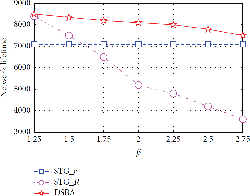
The network lifetime versus β, where the backbone nodes using a large-range radio (or small-range radio) consume β (or $1$ ) energy power for one working cycle; the network has 500 nodes and the initial energy of nodes in the networks is $400$ .

5.2. Size of Virtual Backbone

Figure 6(a) (or Figure 6(b)) shows the simulation results concerning the average nodes of virtual backbones in the networks when the initial energy of each sensor is $400$ (or randomly chosen from the interval $[0,400]$ ). Because the empirical data in Figure 6(b) are similar to those in Figure 6(a), we discuss only the results shown in Figure 6(a). In Figure 6(a), it is clear that the STG $_R$ uses fewer backbone nodes than the DSBA and the STG $_r$ because a large-range radio is used for each backbone node in the STG $_R$ . Although the STG $_R$ has the lowest average number of backbones nodes, the backbone nodes in the STG $_R$ consume much energy power, and, thus, the STG $_R$ often has a shorter network lifetime than the others, as shown in Figures 4 and 5. In addition, note that the more nodes in the networks, the bigger average size of virtual backbones in the DSBA, STG $_r$ , or STG $_R$ is required when the number of nodes is less than or equal to $300$ . This is because more nodes must be dominated, and, thus, more backbone nodes are required. Furthermore, when the number of nodes is greater than $300$ , the empirical data in the DSBA, STG $_r$ , or STG $_R$ are stable and have few differences. This is because the average number of backbone nodes in the DSBA, STG $_r$ , or STG $_R$ is enough to dominate all nodes in the networks.

Figure 6

The average size of virtual backbones versus the number of network nodes ranging from $50$ to $500$ . The initial energies of nodes in the networks are $400$ in (a) and randomly chosen from the interval $[0,400]$ in (b), respectively.

5.3. Residual Energy

Figure 7(a) (or Figure 7(b)) shows the simulation results in terms of the average residual energy of all nodes in the networks when the initial energy of each sensor is $400$ (or randomly chosen from the interval $[0,400]$ ). Because the empirical data in Figure 7(b) are similar to those in Figure 7(a), we discuss only the results shown in Figure 7(a). In Figure 7(a), it is clear that the DSBA has lower average residual energy of all nodes in the networks than STG $_r$ and STG $_R$ . This is because more nodes are selected to be the backbone nodes whose energies are fully utilized to prolong the network lifetime. In addition, when the number of nodes in the networks increases, the average residual energy of all nodes in the network in the DSBA, STG $_r$ , or STG $_R$ appears to decrease. This is because more nodes can be selected to be backbone nodes in the DSBA, STG $_r$ , or STG $_R$ , and, thus, the network lifetime is prolonged, as shown in Figure 4.

Figure 7

The average residual energy of all nodes in the networks versus the number of network nodes ranging from $50$ to $500$ . The initial energies of nodes in the networks are $400$ in (a) and randomly chosen from the interval $[0,400]$ in (b), respectively.

5.4. Number of Virtual Backbones

Figure 8(a) (or Figure 8(b)) shows the simulation results in terms of the average number of virtual backbones when the initial energy of each sensor is $400$ (or randomly chosen from the interval $[0,400]$ ). Because the empirical data in Figure 8(b) are similar to those in Figure 8(a), we discuss only the results shown in Figure 8(a). In Figure 8(a), it is clear that the DSBA has higher average number of virtual backbones than STG $_r$ and STG $_R$ . This is because the DSBA can use a small-range or large-range radio to form the virtual backbones, and thus, the average number of virtual backbones is increased. In addition, when the number of nodes in the networks increases, the average number of virtual backbones in the networks in the DSBA, STG $_r$ , or STG $_R$ appears to increase. This is because more nodes can be selected to be backbone nodes in the DSBA, STG $_r$ , or STG $_R$ , and, thus, the average number of virtual backbones is increased.

Figure 8

The average number of virtual backbones versus the number of network nodes ranging from $50$ to $500$ . The initial energies of nodes in the networks are $400$ in (a) and randomly chosen from the interval $[0,400]$ in (b), respectively.

6. Conclusion

In this paper, while considering sensors each equipped with two radio interfaces, including small-range and large-range radios, a new problem, called the Maximum Lifetime Backbone Scheduling for Dual-Radio Wireless Sensor Network problem, is introduced for finding virtual backbones to prolong the network lifetime. The Maximum Lifetime Backbone Scheduling for Dual-Radio Wireless Sensor Network problem proved to be NP-complete. Moreover, because centralized algorithms are not feasible in a wide range of wireless sensor networks, we propose a distributed algorithm, called the Dominating-Set-Based Algorithm (DSBA), to find a backbone when a new backbone is required for the network. In the DSBA, three steps are required. In the first step, the distributed dominating set algorithm (DDSA) is proposed to construct a dominating set for a given dual-radio wireless sensor network such that the nodes in the set have enough energy power to be the backbone nodes and can dominate all nodes in the network. In the second step, the distributed backbone algorithm (DBA) is proposed to establish a backbone according to the dominating set constructed by the DDSA. In the third step, the refinement for the generated backbone is proposed to minimize the size of the generated backbone or reduce the energy consumption of backbone nodes.

In the simulations, we compared our proposed method with the STG [15] that is a centralized algorithm and is used to find the virtual backbones in the network with sensors each having a single radio. The STG that used a small-range radio (or large-range radio) to construct virtual backbones was adopted and denoted by STG $_r$ (or STG $_R$ ). The performance was evaluated in terms of the network lifetime, the average size of the constructed virtual backbones, the average residual energy of sensors, and the average number of virtual backbones. Simulation results showed that our proposed method had a significantly longer network lifetime and the lower average residual energy of sensors than STG $_r$ and STG $_R$ .

Planned future research will include research in routing in multiradio mobile wireless sensor networks. Other future research will study the routing in three-dimensional multiradio wireless sensor networks.

Footnotes

Conflict of Interests

The authors declare that there is no conflict of interests regarding the publication of this paper.

Acknowledgement

This work was supported by the Ministry of Science and Technology under Grants MOST 103-2221-E-151-002 and MOST 104-2221-E-151-014.

References

Mehmood

Khan

Shams

Lloret

Energy-efficient multi-level and distance-aware clustering mechanism for WSNs

International Journal of Communication Systems 2015 28 5 972 989

10.1002/dac.2720

2-s2.0-84923216103

Shi

Yao

Zhang

An efficient distributed routing protocol for wireless sensor networks with mobile sinks

International Journal of Communication Systems 2015 28 11 1789 1804

10.1002/dac.2785

2-s2.0-84899039343

Akkaya

Younis

Energy-aware delay-constrained routing in wireless sensor networks

International Journal of Communication Systems 2004 17 6 663 687

10.1002/dac.673

2-s2.0-4444379401

Wang

Chua

K. C.

Srinivasan

Connected sensor cover for area information coverage in wireless sensor networks

International Journal of Communication Systems 2008 21 11 1181 1203

10.1002/dac.946

2-s2.0-55349094689

Chen

H.-H.

Deng

D.-J.

Cheng

R.-S.

Chilamkurti

Recent issues in wireless sensor networks

International Journal of Communication Systems 2013 26 9 1089 1091

10.1002/dac.2617

2-s2.0-84883172279

Wang

Y.-C.

F.-J.

Tseng

Y.-C.

Mobility management algorithms and applications for mobile sensor networks

Wireless Communications and Mobile Computing 2012 12 1 7 21

10.1002/wcm.886

2-s2.0-84855172007

Hwang

S.-F.

K.-H.

Y.-Y.

Hsien

C.-S.

Dow

C.-R.

Hierarchical multicast in wireless sensor networks with mobile sinks

Wireless Communications and Mobile Computing 2012 12 1 71 84

10.1002/wcm.890

2-s2.0-84855176956

Martins

Shen

Determination method of optimal number of clusters for clustered wireless sensor networks

Wireless Communications and Mobile Computing 2012 12 2 158 168

10.1002/wcm.949

2-s2.0-84862933446

Cheng

Ding

D. H.

Jia

Virtual backbone construction in multihop ad hoc wireless networks

Wireless Communications and Mobile Computing 2006 6 2 183 190

10.1002/wcm.378

2-s2.0-33645521024

10.

Wang

X.-Y.

Efficient distributed low-cost backbone formation for wireless networks

IEEE Transactions on Parallel and Distributed Systems 2006 17 7 681 693

10.1109/TPDS.2006.86

2-s2.0-33745686736

11.

Dai

Virtual backbone construction in MANETs using adjustable transmission ranges

IEEE Transactions on Mobile Computing 2006 5 9 1188 1199

10.1109/tmc.2006.140

2-s2.0-33746928443

12.

Chuang

S.-Y.

Chen

SmartBone: an energy-efficient smart backbone construction in wireless sensor networks

Proceedings of the IEEE Wireless Communications and Networking Conference (WCNC ′07)

March 2007

Kowloon, China

IEEE

3394 3399

10.1109/wcnc.2007.624

2-s2.0-36349017864

13.

Zhang

Wang

Xin

A new performance metric for construction of robust and efficient wireless backbone network

IEEE Transactions on Computers 2012 61 10 1495 1506

10.1109/TC.2011.185

2-s2.0-84865678649

14.

Torkestani

J. A.

Backbone formation in wireless sensor networks

Sensors and Actuators A: Physical 2012 185 117 126

10.1016/j.sna.2012.06.032

2-s2.0-84865604812

15.

Zhao

On maximizing the lifetime of wireless sensor networks using virtual backbone scheduling

IEEE Transactions on Parallel and Distributed Systems 2012 23 8 1528 1535

10.1109/TPDS.2011.305

2-s2.0-84863510617

16.

Kunz

Tatham

Localization in wireless sensor networks and anchor placement

Journal of Sensor and Actuator Networks 2012 1 1 36 58

10.3390/jsan1010036

17.

Munishwar

V. P.

Abu-Ghazaleh

N. B.

Coverage algorithms for visual sensor networks

ACM Transactions on Sensor Networks 2013 9 4, article 45

10.1145/2489253.2489262

2-s2.0-84893905289

18.

Canthadai

A. M.

Radhakrishnan

Sarangan

Multi-radio wireless sensor networks: energy efficient solutions for radio activation

Proceedings of the 53rd IEEE Global Communications Conference (GLOBECOM ′10)

December 2010

IEEE

1 5

10.1109/glocom.2010.5683413

2-s2.0-79551631279

19.

Jung

Savvides

An energy efficiency evaluation for sensor nodes with multiple processors, radios and sensors

Proceedings of the 27th Conference on Computer Communications (INFOCOM ′08)

April 2008

IEEE

20.

Lymberopoulos

Priyantha

N. B.

Goraczko

Zhao

Towards energy efficient design of multi-radio platforms for wireless sensor networks

Proceedings of the International Conference on Information Processing in Sensor Networks (IPSN ′08)

April 2008

257 268

10.1109/ipsn.2008.51

2-s2.0-51249120571

21.

Moon

S.-H.

Han

S.-J.

Benefits of dual-radio wireless sensor networks

Proceedings of the 7th IEEE Consumer Communications and Networking Conference (CCNC ′10)

January 2010

Las Vegas, Nev, USA

IEEE

1 2

10.1109/ccnc.2010.5421781

2-s2.0-77951263457

22.

Sharma

T. P.

Joshi

R. C.

Misra

Dual radio based cooperative caching for wireless sensor networks

Proceedings of the 16th International Conference on Networks (ICON ′08)

December 2008

1 7

10.1109/icon.2008.4772565

2-s2.0-66649134383

23.

Kim

Jeong

Han

S.-J.

Experimental analysis of interference in dual-radio wireless sensor networks

Proceedings of the 7th IEEE Consumer Communications and Networking Conference (CCNC ′10)

January 2010

1 2

10.1109/ccnc.2010.5421757

2-s2.0-77951289725

24.

Jaikaeo

Shen

C.-C.

Adaptive backbone multicast routing for mobile ad hoc networks

Wireless Communications and Mobile Computing 2008

John Wiley & Sons

25.

Jiao

Lou

Cao

Wang

Zhou

Minimum latency broadcast scheduling in duty-cycled multihop wireless networks

IEEE Transactions on Parallel and Distributed Systems 2012 23 1 110 117

10.1109/TPDS.2011.106

2-s2.0-82555186943

26.

Xiong

Wang

Liu

Multiple task scheduling for low-duty-cycled wireless sensor networks

Proceedings of the 30th IEEE International Conference on Computer Communications (INFOCOM ′11)

April 2011

Shanghai, China

IEEE

1323 1331

10.1109/INFCOM.2011.5934916

27.

Lymberopoulos

Priyantha

N. B.

Goraczko

Zhao

Towards energy efficient design of multi-radio platforms for wireless sensor networks

Proceedings of the 7th International Conference on Information Processing in Sensor Networks (IPSN ′08)

April 2008

Washington, DC, USA

IEEE Computer Society

257 268

10.1109/ipsn.2008.51

2-s2.0-51249120571

28.

Campbell

C. E.-A.

Khan

Singh

Loo

K.-K.

Multi-channel multi-radio using 802.11 based media access for sink nodes in wireless sensor networks

Sensors 2011 11 5 4917 4942

10.3390/s110504917

2-s2.0-79957711090

29.

Jia

Rajaraman

Suel

An efficient distributed algorithm for constructing small dominating sets

Distributed Computing 2002 15 4 193 205

10.1007/s00446-002-0078-0

2-s2.0-0036935239

30.

Schaudt

Schrader

The complexity of connected dominating sets and total dominating sets with specified induced subgraphs

Information Processing Letters 2012 112 24 953 957

10.1016/j.ipl.2012.09.002

MR2979503

2-s2.0-84866050784

31.

Wang

Connected dominating sets in wireless ad hoc and sensor networks a comprehensive survey

Computer Communications 2013 36 2 121 134

10.1016/j.comcom.2012.10.005

2-s2.0-84871418616

32.

Kim

Zou

D.-Z.

Constructing minimum connected dominating sets with bounded diameters in wireless networks

IEEE Transactions on Parallel and Distributed Systems 2009 20 2 147 157

10.1109/tpds.2008.74

An Efficient Algorithm of Constructing Virtual Backbone Scheduling for Maximizing the Lifetime of Dual-Radio Wireless Sensor Networks

Abstract

1. Introduction

2. System Model and Problem Definition

2.1. System Model

2.2. Problem Definition and Its Hardness

Theorem 1.

Proof.

3. The Dominating-Set-Based Algorithm (DSBA)

Definition 2.

3.1. Construction of Dominating Set

Algorithm 1: DDSA ( v ) .

3.2. Establishment of Backbone

Algorithm 2: DBA ( v ) .

3.3. Refinement of Backbone

Rule 1.

Rule 2.

4. Analysis of the DSBA

Lemma 3.

Proof.

Lemma 4.

Proof.

Lemma 5.

Proof.

Theorem 6.

Proof.

5. Performance Evaluation

5.1. Network Lifetime

5.2. Size of Virtual Backbone

5.3. Residual Energy

5.4. Number of Virtual Backbones

6. Conclusion

Footnotes

Conflict of Interests

Acknowledgement

References

Algorithm 1: $DDSA (v)$ .

Algorithm 2: $DBA (v)$ .