Precise Relative Positioning of Vehicles with On-the-Fly Carrier Phase Resolution and Tracking

Abstract

Forward collision warning systems, lane change assistants, and cooperative adaptive cruise control are examples of safety relevant applications that rely on accurate relative positioning between vehicles. Current solutions estimate the position of an in-front driving vehicle by measuring the distance with a radar sensor, a laser scanner, or a camera system. The perception range of these sensors can be extended by the exchange of GNSS information between the vehicles using an intervehicle communication link. One possibility is to transmit GNSS pseudorange and carrier phase measurements and compute a highly accurate baseline vector that represents the relative position between two vehicles. Solving for the unknown integer ambiguity is specially challenging for low-cost single-frequency receivers. Using the well-known LAMBDA (Least-squares AMBiguity Decorrelation Adjustment) algorithm, in this paper, we present a method for tracking the ambiguity vector solution, which is able to detect and recover from cycle slips and cope with changing satellite constellations. In several test runs performed in real-world open-sky environments with two vehicles, the performance of the proposed Ambiguity Tracker approach is evaluated. The experiments revealed that it is in fact possible to track the position of another vehicle with subcentimeter accuracy over longer periods of time with low-cost single-frequency receivers.

1. Introduction

To make transportation more efficient and safer, today's vehicles are already equipped with multiple Advanced Driver Assistance Systems. Forward collision warning systems, lane change assistants, and adaptive cruise control are safety related applications that require a highly accurate relative position to other vehicles. Today, these systems completely rely on on-board ranging sensors to estimate the position towards surrounding traffic participants. Radar sensors, laser scanners, and vision-based systems offer a good relative position and relative velocity estimation to other vehicles. These sensors, however, exhibit a series of important limitations. While long-range radar sensors can measure the distance to other vehicles up to 200 m, laser scanners have lower sensing ranges. Cameras have a range limitation due to the limited distance between cameras in stereovision systems or due to pixel resolution in monocular systems. All of these systems have also an accuracy degradation with ranging distance. However, more important than the limited ranging capabilities are their line-of-sight characteristic. All of them are not able to estimate the position of vehicles behind other vehicles, behind bends and crests, or around buildings.

The key approaches to solve these limitations and to extend the awareness range of future intelligent vehicles are cooperative approaches based on vehicle-to-vehicle communication. In recent years, big steps in the standardization of intervehicle communication have been achieved in Europe, North America, and Japan. By transmitting special beaconing messages, in near future, vehicles will be able to provide position information to their neighbors to create mutual awareness up to a range of several hundreds of meters. In this context, the basis for localization is Global Navigation Satellite Systems (GNSS) as the American GPS, the Russian GLONASS, or the European Galileo system. In [1], the authors presented a cooperative approach based on the exchange of GNSS pseudoranges and the estimation of the relative position between two vehicles.

In this work, we want to extend the concept of exchanging GNSS pseudorange measurements, by additionally exchanging GNSS carrier phase measurements between vehicles. As opposed to pseudorange measurements, carrier phase measurements are around two orders of magnitude more precise and have the potential of achieving subcentimeter precise range to a neighboring vehicle. However, carrier phase measurements come along with an inherent integer unknown and are highly sensitive to signals losses and obstructions. Cycle slips are discontinuities in the cycle count that heavily degrade the performance of carrier phase positioning solutions.

Real-Time Kinematic (RTK) is an approach to solve the absolute position of a moving receiver in real time using a precisely surveyed base station. In automotive environments, this technique is often used as a position ground truth during experiments [2, 3]. For this purpose, usually expensive high-end GNSS receivers with specially designed antennas to reduce the impact of multipath propagation are used.

A number of groups have addressed the relative positioning problem of vehicles by solving differenced carrier phase ambiguities rather than using differenced pseudorange techniques. Ansari et al. have investigated cooperative relative positioning by exchanging RTK position solutions between vehicles [4]. Their system also uses high-graded GNSS receivers and a connection to a roadside unit delivering GPS correction data. Basnayake et al. [5] built a test platform for relative positioning yielding range errors of less than 1 m 99% of the time in open sky and 90% on obscured roads. Travis et al. [6, 7] have worked on a trajectory duplication using carrier phase based relative positioning. They perform a direct exchange of the measurements between the receivers to compute single differences and estimate the relative position by incorporating inertial measurements. They also use high-end receivers and do not address the problem of cycle slips.

Takasu and Yasuda worked on cycle-slip detection in automotive environments using dual-frequency high-graded receivers [8]. They propose an integration of GNSS and inertial sensor inside a Kalman filter to exploit the complementary nature of both sensors. A Bayesian approach to cope with cycle slips and changing satellite constellation is proposed by Zeng et al. [9].

It is expected that vehicles will be rather equipped with low-cost single-frequency receivers than dual-frequency, geodetic graded receivers. Unfortunately, such low-cost receivers are less precise and suffer more often from losses of lock. The automotive scenario is specially challenging regarding the usage of GNSS, due to the presence of plenty of obstacles above and next to the road. These obstacles in a highly dynamic environment will produce often such loss of lock. Henkel and Iafrancesco work on carrier phase solutions in vehicular environments for attitude determination using low-cost receivers and sensor fusion by using multiple antennas on the roof of a vehicle [10]. Kiam et al. propose a Kalman filter solution without additional sensors by exploiting the movement model of nodes carrying the receivers [11].

In this work, we analyze the possibility of only using low-cost single-frequency GPS receivers to precisely estimate the baseline between two vehicles by solving the integer ambiguity in the carrier phase measurements. A new approach, the Ambiguity Tracker, is described in the next section. To find the correct integer ambiguity vector multiple Ambiguity Trackers are run in parallel and weighted according to certain parameters. This approach is explained in Section 3. A Baseline Tracking Filter is presented in Section 4. The Ambiguity Tracker approach is evaluated in real-world experiments described in Section 5. The paper ends with the conclusions in Section 6.

2. Ambiguity Tracker

A GNSS receiver is able to compute a position by estimating the range towards at least four satellites. The estimate of the range towards a satellite is called pseudorange and it is corrupted by several types of errors. The model for a pseudorange measurement ${\rho }_e^l$ from a receiver e to a satellite l is

$$\begin{array}{cc}& {\rho }_e^l=r_e^l+c·\left(\delta t_e-\delta t^l\right)+I+T+E+M+{ϵ}_{\rho },\end{array}$$

(1)

where $r_e^l$ is the true range towards the satellite, c is the speed of light, $\delta t_e$ is the receiver clock bias, $\delta t^l$ is the satellite clock bias, and I, T, and E are the ionospheric delay, the tropospheric delay, and satellite position error, respectively. These errors are strongly correlated between close-by receivers. M is the range estimation error due to multipath propagation and ${ϵ}_{\rho }$ contains all nonmodeled errors such as receiver noise.

The carrier phase measurement can be expressed in the following way:

$$\begin{array}{cc}& {\varphi }_e^l=r_e^l+c·\left(\delta t_e-\delta t^l\right)-I+T+E+M+\lambda ·N_e^l+{ϵ}_{\varphi },\end{array}$$

(2)

where λ is the L1 wavelength and $N_e^l$ corresponds to the integer number of cycles between the satellite and the receiver. Further information regarding GNSS satellite acquisition and tracking and GNSS measurements and its errors can be found in [12].

Double differences are computed in order to cancel out some of the previously stated errors on the pseudoranges and the carrier phase measurements. In a first step, the pseudoranges ${\rho }_e^l$ and ${\rho }_t^l$ towards the same satellite at two receivers e and t are subtracted to yield a single difference $\Delta {\varphi }_{et}^l$ . With this approach the errors common to both receivers, such as satellite clock errors and ephemeris errors, are canceled out directly. In this use case, unlike RTK, the distance between the antennas is below 1 km, and under this assumption, full correlation of ionospheric and tropospheric errors can be assumed. It is true, however, that extreme ionospheric storms can lead to ionospheric delay gradients above 400 mm/km, making the fixing of carrier phase ambiguities practically impossible [13]. Also sudden variations in the concentration of water vapor in the lower troposphere can, in rare cases, cause a difference between the tropospheric delays at different locations. Measurements with 2 to 3 km baselines yielded differences in the tropospheric error of around 3 cm [14]. However, these events are rather seldom and, therefore, in this work we assume a sufficient correlation between the ionospheric and tropospheric delays at both ego and target vehicle and a perfect cancellation of their impact by means of double differences.

A synchronization procedure prior to the subtraction of two pseudorange measurements to yield a single difference is required in order to bring the measurements to a common point in time [15]. For this, both the pseudoranges and the carrier phase measurements are extrapolated using the current Doppler according to

$$\begin{array}{cc}& {\rho }_e^l\left(t_e+\Delta t\right)={\rho }_e^l\left(t_e\right)+\Delta t·\lambda ·{\dot{\varphi }}_e^l\left(t_e\right),\\ {\varphi }_e^l\left(t_e+\Delta t\right)={\varphi }_e^l\left(t_e\right)+\Delta t·\lambda ·{\dot{\varphi }}_e^l\left(t_e\right),\end{array}$$

(3)

where ${\dot{\varphi }}_e^l$ is the Doppler measurement from receiver e to satellite l, $t_e$ is the time instant when receiver e made the measurement (corrected by the receiver clock bias), and $\Delta t$ is the time difference to the common time instant agreed between the ego and target vehicle. This synchronization procedure yields good results as long as the relative movement between receiver and satellite is uniform in the extrapolation time $\Delta t$ .

Here, we want to take the opportunity to point out the importance of possible system delays for a real-time application. The time required for transferring the target vehicle's GNSS measurements to the ego vehicle, including processing at the receiver and the on-board computer, message composition, modulation, channel access, transmission, demodulation, and processing, will cause the estimation of the relative position of the target vehicle in the ego vehicle to lag behind the actual position. The quantification of this delay and its implication on a real-time driver assistance application falls out of the scope of this work and is left as an important aspect to be regarded.

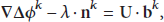
By subtracting two single differences towards satellites l and m, a double difference that cancels also the receiver clock biases in e and t is composed. A pseudorange double difference $\nabla \Delta {\rho }_{et}^{lm}$ is a projection of the baseline b between both antennas towards the difference in unitary vectors ${\mathbf{u}}^m-{\mathbf{u}}^l$ . Hence, the following system of linear equations can be composed:

$$\begin{array}{cc}& \mathbf{\nabla }\mathbf{\Delta }\mathit{\rho }=\mathbf{U}·\mathbf{b}+\mathbf{\nabla }\mathbf{\Delta }{\mathit{ϵ}}_{\rho },\end{array}$$

(4)

where U is the matrix containing the differenced unitary vectors u as row vectors and $\mathbf{\nabla }\mathbf{\Delta }{\mathit{ϵ}}_{\rho }$ contains the noncanceled errors, that is, pseudorange noise and multipath errors. By taking $p\ge \mathrm{3}$ double differences the baseline between the vehicles can be solved. Analogous to pseudoranges, double differences from carrier phase measurements $\nabla \Delta {\varphi }_{et}^{lm}$ can be created. These contain the double differenced integer ambiguity $\nabla \Delta N_{et}^{lm}$ . Therefore, the resulting system of linear equations contains not only the three unknowns of the baseline vector b, but also a vector of double differenced integer ambiguities n:

$$\begin{array}{cc}& \mathbf{\nabla }\mathbf{\Delta }\mathit{\varphi }-\lambda ·\mathbf{n}=\mathbf{U}·\mathbf{b}+\mathbf{\nabla }\mathbf{\Delta }{\mathit{ϵ}}_{\varphi }.\end{array}$$

(5)

The system of linear equations with p carrier phase double differences contains $p+\mathrm{3}$ unknowns, of which the baseline b is a vector of real numbers and the ambiguity n a vector of integers. Moreover, the variance-covariance matrix of $\mathbf{\nabla }\mathbf{\Delta }{\mathit{ϵ}}_{\varphi }$ is highly elongated. A brute force approach that finds the integer ambiguity vector n that minimizes the residual error $\mathbf{\nabla }\mathbf{\Delta }{\mathit{ϵ}}_{\varphi }$ is usually impractical. The LAMBDA (Least-squares AMBiguity Decorrelation Adjustment) method developed by Teunissen [16] is a well-known algorithm to effectively estimate the integer ambiguities. Taking p pseudorange and p carrier phase measurements in (4) and (5), a float solution ${\widehat{\mathbf{n}}}_f$ for the integer ambiguities is found. By performing a Z-transformation, the highly elongated search space is decorrelated and an integer search near the transformed float solution can efficiently be performed. The found integer ambiguity is transformed back to give the fixed integer ambiguity $\check{\mathbf{n}}$ . Using (5) the fixed baseline $\check{\mathbf{b}}$ is computed.

The performance of the LAMBDA method is strongly dependent on the correct selection of the measurement covariance matrix. In this work the estimated carrier-to-noise ratio by the receiver is taken to compute the variance-covariance matrices of $\mathbf{\nabla }\mathbf{\Delta }{\mathit{ϵ}}_{\rho }$ and $\mathbf{\nabla }\mathbf{\Delta }{\mathit{ϵ}}_{\varphi }$ . The relationship between the carrier-to-noise ratio and the pseudorange double differences noise for the used GPS receivers is assessed in [15].

The LAMBDA method, as described here, is performed at each epoch. Errors in both, pseudoranges and carrier phase measurements, will, in practice, cause the correct integer ambiguity to be not the first solution given by the LAMBDA algorithm. However, these errors will average over time and eventually the ambiguity can be fixed with high confidence.

Cycle slips are losses of the carrier phase count inside the phase-lock loop (PLL). They are caused by momentary loss of signal strength due to satellite line-of-sight obstruction or multipath-induced fading. Usually, the reacquisition of the carrier phase measurements takes less than one second. Often, a half wave length ambiguity remains, which is not resolved until two consecutive navigation data subframes are received [8]. These so-called half-cycle slips need 8–12 s to be resolved. Cycle slips cause the computation of the integer ambiguity to be reset and are the main reason for the unavailability of a carrier phase solution in automotive environments.

In static conditions, the detection of cycle slips on carrier phase double differences is simple, due to the discrete step of a few centimeters in the measurements. In dynamic conditions, however, a jump in the double difference carrier phase signal remains undetected. The change in carrier phase double difference between two measurements taken at 4 Hz of two vehicles with a speed difference of 10 m/s is 2.5 m. Compared to a half-cycle slip of around 9 cm the change due to the movement of the vehicles is much greater.

In this work a new algorithm to track the integer ambiguity vector over time withstanding the occurrence of cycle slips and attaining for changes in the satellite constellation is presented. The Ambiguity Tracker is once initialized using the LAMBDA method and from then on it will track the resulting ambiguity vector over time by detecting cycle slips and half-cycle slips. The following five steps along with the flow diagram in Figure 2 describe the procedure of the Ambiguity Tracker.

(a) Initialization. The previously described LAMBDA method is used to compute an integer ambiguity vector ${\check{\mathbf{n}}}^{\mathrm{0}}$ and a fixed baseline solution ${\check{\mathbf{b}}}^{\mathrm{0}}$ from the current pseudorange and carrier phase double difference measurements.

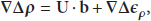
(b) Cycle-Slip Detection. Cycle slips on the carrier phase measurements in epoch k are detected by first predicting the baseline in step k from the baseline, baseline velocity, and baseline acceleration in step $k-\mathrm{1}$ according to

$$\begin{array}{cc}& {\widehat{\mathbf{b}}}^k={\mathbf{b}}^{k-\mathrm{1}}+{\dot{\mathbf{b}}}^{k-\mathrm{1}}·\Delta t+\frac{\mathrm{1}}{\mathrm{2}}·{\ddot{\mathbf{b}}}^{k-\mathrm{1}}·\Delta t^{\mathrm{2}},\end{array}$$

(6)

where

$$\begin{array}{cc}& {\dot{\mathbf{b}}}^{k-\mathrm{1}}=\frac{{\mathbf{b}}^{k-\mathrm{1}}+{\mathbf{b}}^{k-\mathrm{2}}}{\Delta t},\\ {\ddot{\mathbf{b}}}^{k-\mathrm{1}}=\frac{{\dot{\mathbf{b}}}^{k-\mathrm{1}}+{\dot{\mathbf{b}}}^{k-\mathrm{2}}}{\Delta t},\end{array}$$

(7)

and $\Delta t$ is the time between GNSS measurements. In a second step the integer ambiguity for the predicted baseline ${\widehat{\mathbf{n}}}^k$ is computed with

$$\begin{array}{cc}& {\widehat{\mathbf{n}}}^k=\frac{\mathbf{\nabla }\mathbf{\Delta }{\mathit{\varphi }}^k-\mathbf{u}·{\widehat{\mathbf{b}}}^k}{\lambda }-\frac{\mathbf{\nabla }\mathbf{\Delta }{\mathit{ϵ}}_{\varphi }^k}{\lambda }.\end{array}$$

(8)

This predicted ambiguity is compared to that of the previous step ${\widehat{\mathbf{n}}}^{k-\mathrm{1}}$ . The difference $r={\widehat{\mathbf{n}}}^k-{\widehat{\mathbf{n}}}^{k-\mathrm{1}}$ will ideally yield zero if no cycle slip occurred. However, due to errors in the prediction and due to noise in the carrier phase measurements, a suitable threshold for r should be selected. If the threshold is selected too wide, some cycle slips might stay undetected, while if it is selected too tight prediction errors and carrier phase noise will lead to faulty cycle-slips detection and reduction of tracked satellites. The loss of messages from the target vehicle due to blockage, fading, or message collisions will have a detrimental impact on the performance of the cycle-slip detector, since $\Delta t$ increases and prediction errors grow.

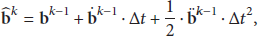
(c) Baseline Computation. The baseline ${\mathbf{b}}^k$ is computed by solving

$$\begin{array}{cc}& \mathbf{\nabla }\mathbf{\Delta }{\mathit{\varphi }}^k-\lambda ·{\mathbf{n}}^k=\mathbf{U}·{\mathbf{b}}^k,\end{array}$$

(9)

where the ambiguities ${\mathbf{n}}^k$ are already known from the previous epoch ( ${\mathbf{n}}^k={\mathbf{n}}^{k-\mathrm{1}}$ ). The best solution to (9) in a minimum mean squared error sense is given the least squares solution

$$\begin{array}{l}{\mathbf{b}}^k={\left({\mathbf{U}}^T·{\mathbf{Q}}_{\nabla \Delta \varphi }^{-\mathrm{1}}·\mathbf{U}\right)}^{-\mathrm{1}}·{\mathbf{U}}^T·{\mathbf{Q}}_{\nabla \Delta \varphi }^{-\mathrm{1}}\\ \hspace{1em}·\left(\mathbf{\nabla }\mathbf{\Delta }{\mathit{\varphi }}^k-\lambda ·{\mathbf{n}}^k\right),\end{array}$$

(10)

where ${\mathbf{Q}}_{\nabla \Delta \varphi }$ is the variance-covariance matrix of the carrier phase double difference measurements.

(d) Quarantine. Carrier phase double differences that are detected to be affected by a cycle slip are placed in the so-called quarantine. This is also the case for newly tracked satellites or satellites that are reacquired after a signal blockage, which are likely to be affected by half-cycle slips that jump back after a few seconds.

(e) Integer Ambiguity Computation. This step tries to compute the integer ambiguity for the satellites placed in quarantine. This is done using the fixed baseline ${\mathbf{b}}^k$ from (10) along with the satellite i carrier phase measurements $\nabla \Delta {\varphi }_i^k$ to compute an estimate

$$\begin{array}{cc}& {\widehat{n}}_i^k=\frac{\nabla \Delta {\varphi }_i^k-{\mathbf{u}}_i·{\mathbf{b}}^k}{\lambda }.\end{array}$$

(11)

Errors in the carrier phase measurements will cause this estimate to be not exactly an integer number. This fact is used to determine whether to remove the satellite from quarantine and incorporate it into the baseline estimation in the next step. If ${\widehat{\mathbf{n}}}_i^k$ is close to an integer the satellite is free from half-cycle slips and can be used in the next step.

It should be noted that an Ambiguity Tracker needs at least four satellites without cycle slips in order to be able to track its baseline solution, the common satellite and three satellites, in order to have three equations. Therefore, if an Ambiguity Tracker tracks three or less satellites without cycle slips, this Ambiguity Tracker is automatically reinitialised.

3. Multiple Ambiguity Hypotheses

As explained in the previous section, the LAMBDA method is used to compute an integer ambiguity vector from pseudorange and carrier phase measurements, which is used to initialize the Ambiguity Tracker. The success of the approach depends on the ability of single-epoch LAMBDA to find the correct ambiguity. Unfortunately, the success rates for low-cost single-frequency receivers are not higher than 40% [17].

A real-world test was performed with a static known 2.131 m baseline over a period of five minutes. The LAMBDA method was used to output its first 5 ambiguity vector candidates. Table 1 summarizes the percentage of hits of the correct ambiguity vector in the different candidates depending on the number of tracked satellites. Tracking eight satellites LAMBDA was always able to find the correct ambiguity vector on the first candidate. However, the fewer the satellites used are, the more the true ambiguity vector is spread over the different candidates. With five satellites, for instance, in less than 20% of the epochs, the correct ambiguity was found on one of the five first candidates. This limits the use of a single Ambiguity Tracker, since the likelihood of initializing with the correct ambiguity is strongly reduced with decreasing number of tracked satellites. In near future, receivers capable of tracking multiple constellation, as GLONASS and Galileo, are expected to enter the mass market, making the success rates of single-epoch ambiguity LAMBDA increase [18]. Still the problem persists in partially obstructed environments or single-constellation receivers.

Table 1

LAMBDA method performance.

Number of satellites	Correct ambiguity in candidate
	1st	2nd	3rd	4th	5th
3	0.49%	0.37%	0.33%	0.17%	0.26%
4	0.66%	1.16%	1.82%	0.99%	2.15%
5	3.63%	5.44%	2.97%	3.13%	4.29%
6	49.43%	24.22%	14.83%	7.75%	1.98%
7	98.68%	1.32%	0%	0%	0%
8	100%	0%	0%	0%	0%

One possibility to overcome this limitation of the single-epoch LAMBDA method is to apply it on successive epochs. Since random errors tend to average, eventually a single candidate ambiguity vector can be regarded to be the correct one. However, this method has to be reset each time a cycle slip occurs. As in automotive environments the probability of cycle slips occurring is high, in this work we do not consider multiepoch LAMBDA method but stick to the single-epoch approach. We propose to run several Ambiguity Trackers in parallel, each of them tracking a different ambiguity vector n. Each Ambiguity Tracker represents a hypothesis on the baseline between both vehicles. The idea behind this approach is the fact that an incorrect ambiguity vector will eventually yield a large residual error.

With increasing time the wrong ambiguity vectors will yield inconsistent solutions. Figure 3 presents the residual errors for several Ambiguity Trackers each following a different ambiguity vector in the static environment of a 2.131 m baseline in an open-sky environment. The first Ambiguity Tracker AT1 is tracking the correct ambiguity. It can be observed how the residual errors of the other Ambiguity Trackers grow steadily until they are reset.

Running multiple Ambiguity Trackers in parallel consists of three steps. First, new Ambiguity Trackers need to be created. Second, the Ambiguity Trackers need to be weighted according to some parameter that will eventually find the correct solution. Finally, the Ambiguity Tracker with the highest weight is selected to be the fixed or correct baseline solution.

3.1. Ambiguity Tracker Creation

To create P new Ambiguity Trackers, the first P integer ambiguity solutions of LAMBDA method taking the current measurements at time step k are considered. Each Ambiguity Tracker follows its integer ambiguity over time according to the steps explained in Section 2. An Ambiguity Tracker has a weight associated with it and all weights sum to one. In the first step, all P Ambiguity Trackers are initialized to a weight of $\mathrm{1}/P$ . In any later step, a newly created Ambiguity Tracker gets a weight equal to $\mathrm{1}/P$ by taking $\mathrm{1}/P(P-\mathrm{1})$ weight from the existing Ambiguity Trackers.

3.2. Ambiguity Tracker Weighting

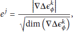
The previous analysis of the residual error suggests that this parameter can be used to weight each Ambiguity Tracker. In each epoch the residual error $\mathbf{\nabla }\mathbf{\Delta }{\mathit{ϵ}}_{\varphi }^k$ is calculated by inserting the measured carrier phase $\mathbf{\nabla }\mathbf{\Delta }{\mathit{\varphi }}^k$ and using the Ambiguity Tracker's ambiguity vector ${\mathbf{n}}^k$ in (5):

$$\begin{array}{cc}& \mathbf{\nabla }\mathbf{\Delta }{\mathit{ϵ}}_{\varphi }^k=\mathbf{\nabla }\mathbf{\Delta }{\mathit{\varphi }}^k-\mathbf{U}·{\mathbf{b}}^k-\lambda ·{\mathbf{n}}^k.\end{array}$$

(12)

The figure of merit to weight each Ambiguity Tracker is the magnitude of the residual error. To compare residual vectors of possibly different dimensions a normalization has to take place according to

$$\begin{array}{cc}& e^j=\frac{\left|\mathbf{\nabla }\mathbf{\Delta }{\mathit{ϵ}}_{\varphi }^k\right|}{\sqrt{\mathrm{d}\mathrm{i}\mathrm{m}\left(\mathbf{\nabla }\mathbf{\Delta }{\mathit{ϵ}}_{\varphi }^k\right)}},\end{array}$$

(13)

where $e^j$ is the normalized weight of the jth Ambiguity Tracker and $\mathrm{d}\mathrm{i}\mathrm{m}(·)$ is the function that yields the dimensionality of a vector.

The number of tracked satellites gives a measure on the likelihood of the ambiguity vector being the correct one. Ambiguity Trackers following incorrect ambiguity vectors will often detect cycle slips and therefore discard satellites measurement.

Hence, both the current residual errors and the number of tracked satellites are used to weight each Ambiguity Tracker.

3.3. Ambiguity Tracker Deletion and Fixing

When the weight of an Ambiguity Tracker falls below a certain value, the Ambiguity Tracker is deleted and replaced by a new one. When the weight of an Ambiguity Tracker exceeds a certain threshold it is highly likely that the integer ambiguity is the correct one and, consequently, the baseline can be said to be fixed.

4. Baseline Tracking Filter

Once the correct solution is found, the baseline solution can be considered as a highly accurate relative positioning. Indeed, using the Ambiguity Tracker approach presented in Section 2, this accurate baseline can be maintained over time without using the LAMBDA method each epoch, avoiding possible wrong ambiguity fixings or float solutions.

However, the Ambiguity Tracker method may lose the tracking of the accurate baseline. A tunnel, a bridge, or even a single tree near the road can cause the situation where the correct solution cannot be further tracked because the lock on the phase towards multiple satellites is lost at the same time. In this case, the process to search again the correct solution is restarted. This search may be improved if the system predicts the baseline evolution. The idea is to give more weight to those Ambiguity Trackers whose baseline coordinates are closer to the predicted baseline. In this way, the system increases its robustness and a solution is found more quickly.

In this section, we present a Baseline Tracking Filter that estimates the baseline, the heading, and the speed of each vehicle.

4.1. Kalman Filter

A Kalman filter is a recursive Bayesian filter for linear Gaussian systems. The Kalman filtering technique consists of two recursive steps: a prediction and an update step. The prediction step is carried out using the following equation:

$$\begin{array}{cc}& {\mathbf{x}}^k=f\left({\mathbf{x}}^{k-\mathrm{1}}\right)+{\mathit{\nu }}^{k-\mathrm{1}},\end{array}$$

(14)

where $f({\mathbf{x}}^{k-\mathrm{1}})$ is the prediction function, which defines the state transition model, and ${\mathit{\nu }}^{k-\mathrm{1}}$ is the prediction model noise. Note that the superscript indicates the instant of time or epoch. Next, the state ${\mathbf{x}}^k$ is updated by the observed data defined by z. This measurement update step is modeled with the following equation:

$$\begin{array}{cc}& {\mathbf{z}}^k=h\left({\mathbf{x}}^k\right)+{\mathit{\eta }}^k,\end{array}$$

(15)

where $h({\mathbf{x}}^k)$ defines the measurement model and ${\mathit{\eta }}^k$ is the measurement noise.

It should be pointed out that the noise vectors, ν and η , are assumed to be zero-mean white Gaussian noise with covariance matrices Q and R, respectively.

4.2. Baseline Tracking Filter Description

The objective of this filter is to predict the evolution of the baseline between the ego and target vehicle, which is defined as a three-dimensional vector expressed in ENU coordinates: $\mathbf{b}={\left[\begin{array}{ccc}{b}_E& b_N& b_U\end{array}\right]}^T$ . For the purpose of our work we are only interested in predicting the east and the north components of the baseline b. The state vector of the proposed Kalman filter is shown next:

$$\begin{array}{cc}& {\mathbf{x}}^k={\left[\begin{array}{cccccc}{b}_E& b_N& {\psi }_e& {\psi }_t& v_e& v_t\end{array}\right]}^T,\end{array}$$

(16)

where ${\psi }_e$ and $v_e$ are the heading and the speed of the ego vehicle and ${\psi }_t$ and $v_t$ are the heading and the speed of the target vehicle. The prediction equation is described by

$$\begin{array}{cc}& x^k=x^{k-\mathrm{1}}+\Delta t·{\dot{x}}^k,\end{array}$$

(17)

where $\Delta t$ is the time between two steps of the filter and the components of ${\dot{x}}^k$ are:

$$\begin{array}{cc}& {\dot{b}}_E^k=\left[v_t^{k-\mathrm{1}}·\sin \left({\psi }_t^{k-\mathrm{1}}\right)-v_e^{k-\mathrm{1}}·\sin \left({\psi }_e^{k-\mathrm{1}}\right)\right]+{{\nu }_b}_E,\\ {\dot{b}}_N^k=\left[v_t^{k-\mathrm{1}}·\cos \left({\psi }_t^{k-\mathrm{1}}\right)-v_e^{k-\mathrm{1}}·\cos \left({\psi }_e^{k-\mathrm{1}}\right)\right]+{{\nu }_b}_N,\\ {\dot{\psi }}_e^k={\nu }_{{\psi }_e},\\ {\dot{\psi }}_t^k={\nu }_{{\psi }_t},\\ {\dot{v}}_e^k={\nu }_{v_e},\\ {\dot{v}}_t^k={\nu }_{v_t},\end{array}$$

(18)

where ${{\nu }_b}_E$ , ${{\nu }_b}_N$ , ${\nu }_{{\psi }_e}$ , ${\nu }_{{\psi }_t}$ , ${\nu }_{v_e}$ , and ${\nu }_{v_t}$ are the prediction noise of each of the state variables. The baseline coordinates are predicted using a motion model based on the previous states, and the speed and the heading of each vehicle. The prediction of the heading and the speed of both vehicles is modeled with the addition of a zero-mean white Gaussian noise.

A GNSS receiver estimates the three-dimensional velocity vector and the clock drift using Doppler or differenced carrier phase measurements, usually inside a Kalman filter. Taking the horizontal component of the three-dimensional velocity vector the speed and the heading of the receiver can be measured. These measurements are used to update our states as

$$\begin{array}{cc}& {\tilde{\psi }}_e^k={\psi }_e^k+{{\eta }_{\psi }}_e,\\ {\tilde{\psi }}_t^k={\psi }_t^k+{{\eta }_{\psi }}_t,\\ {\tilde{v}}_e^k=v_e^k+{{\eta }_v}_e,\\ {\tilde{v}}_t^k=v_t^k+{{\eta }_v}_t,\end{array}$$

(19)

where ${\tilde{\psi }}_e$ and ${\tilde{\psi }}_t$ are the GNSS heading measurements and ${\tilde{v}}_e$ and ${\tilde{v}}_t$ are the speed measurements in the ego and target vehicle, respectively. The variance for the heading noise ${\eta }_{\psi }$ depends on the speed of the vehicle. At higher speed a more precise heading measurement is obtained, while at standstill the heading remains unobserved. The standard deviation of the noise in the speed measurement ${\eta }_v$ is, in such a benign environment, less than 1 cm/s [19].

Since the presented prediction equations are not linear in the state variables an approximation to the Kalman filter has to be implemented. The Extended Kalman filter linearizes the prediction equations using a first order Taylor approximation.

5. Experimental Results

This section will present the real-world tests that assess the performance of the previously introduced Ambiguity Tracker, the Multiple Ambiguity Hypotheses, and the Baseline Tracking Filter.

5.1. Test Setup

The experiments were performed using two test vehicles. The target vehicle driving in front is a Renault Clio, while the ego vehicle behind is a Mercedes G-400 (see Figure 1). Each vehicle is equipped with a Ublox LEA-4T GPS receiver taking measurement at 4 Hz. The receivers output pseudorange, carrier phase, and Doppler measurements, which are logged along with the navigation messages in the Receiver Independent Exchange Format (RINEX) on board of each vehicle. All processing takes place offline.

Figure 1

Real-world experimental setup: ego and target test vehicles in open-sky environment. Each vehicle is equipped with a GNSS receiver and an antenna mounted on its roof. The baseline represents the relative position between both vehicles.

Figure 2

Ambiguity Tracker flow diagram. The LAMBDA method is used to initialize the Ambiguity Tracker. Cycle slips in the carrier phase double differences are detected using a prediction of the baseline. The baseline is fixed using the cycle-slip free measurements. Cycle-slip corrupted measurements and measurements from newly acquired satellites are placed in quarantine, whose ambiguity is later on computed using the fixed baseline.

Figure 3

A comparison of the normalized residuals of five different Ambiguity Trackers for a static baseline in a 1000 s period. The Ambiguity Tracker following the correct integer ambiguity vector (AT1) has the lowest normalized residual.

A magnetic patch antenna from Ublox is placed on the roof of each vehicle. The experiments were performed in a rural open-sky environment in Hurlach, 70 km west of Munich. Single trees next to the road were the only obstacles encountered that could momentarily block the line of sight to the satellites.

As a reference system, we have compared the estimated baseline length to the geometrical distance between the antennas. For this purpose a Leica Disto handheld laser ranging device has been used, which states to have a typical measuring accuracy of ±1 mm up to 120 m. The range measurement was carefully done by not blocking the sky view of the antennas with the measuring device and by correcting with the antenna phase offsets. Also repeated measurements were performed and the average was taken as a ground truth. In this way, with the Disto ranging device we are able to measure the distance between the patch antennas with subcentimeter accuracy in static conditions.

By comparing the measured range with the estimated baseline length of the different Ambiguity Trackers, the correct integer ambiguity vector can be identified in static conditions. As a further validation step, the baseline height difference between the antennas assuming a flat road was compared to the baseline up-coordinate.

In addition, a laser scanner or Light Detection and Ranging (LIDAR) device is used in order to have a rough reference system in motion conditions. For this purpose, an LD-MRS automotive laser scanner from Sick is mounted in the front part of the ego vehicle, specifically above the number plate. The measurement update rate of this reference sensor is 12.5 Hz. This laser scanner can measure a two-dimensional baseline between the front part of the ego vehicle and the rear part of the target vehicle. The geometrical offsets from the GNSS antennas to the laser scanner in the ego vehicle and to the rear part of the vehicle in the target vehicle have been precisely measured prior to the experiments and have been added to the baseline estimation of the laser scanner. As the laser scanner measures the relative position in the body frame of the vehicle and the Ambiguity Tracker works in the East-North-Up (ENU) coordinate system, only the baseline length will be compared. The up-component is not measured by the laser scanner and will present an error when comparing to the three-dimensional baseline of the Ambiguity Tracker. Other possible error sources of the laser scanner are presented in [20].

5.2. Ambiguity Tracker and Cycle-Slip Detector

The correct tracking of an ambiguity vector is tested in a 200 s run. First, both vehicles are at a standstill at approximately 8 m distance; then they start accelerating up to 40 km/h and drive at changing distances from 5 to 20 m and finally decelerate to standstill. The baseline is accurately measured with the Disto device at the beginning and at the end of the run. Figure 4 displays the pseudorange and carrier phase double differences to all tracked satellites. The higher noise and the effect of multipath can be observed on the pseudoranges in Figure 4(a), while Figure 4(b) reveals the high number of carrier phase losses of lock and consequent cycle slips. Other cycle slips cannot be detected by mere visual inspection since they are masked by the dynamics of the baseline during the run.

Figure 4

Pseudorange and carrier phase double differences for 13 satellites in view during a 200-second run. At the beginning and at the end of the run the vehicles are at standstill.

One single Ambiguity Tracker is initialized with the correct integer ambiguity vector, which has been determined by applying LAMBDA successively to the 30 s initial standstill time, calculating the baseline for all most probable candidates, and comparing its length to the reference distance. To determine whether the Ambiguity Tracker is able to correctly follow the integer ambiguity vector with changing satellite constellations and the multiple cycle slips, the baseline length of the Ambiguity Tracker and the references measured by the Disto device at the beginning and at the end of the run are shown in Figure 5. An error of 3 mm and 2 mm is measured, respectively. Moreover, Figure 6 shows how the baseline length tracked by the Ambiguity Tracker matches the LIDAR reference. We can conclude that the Ambiguity Tracker did successfully track the ambiguity during the 200 s run. Figure 6 also shows the baseline length from the Ambiguity Tracker compared to the pseudorange solution. Meter-level errors of the pseudorange baseline solution can be observed during standstill and while driving.

Figure 5

Baseline length estimated by the Ambiguity Tracker (green) and measured with Disto handheld laser ranging device (blue) at the beginning and at the end of a 200-second run. The errors of a few millimeters indicate that the correct integer ambiguity vector is tracked.

Figure 6

A comparison between the baseline length based on the pseudorange measurements (orange) and the baseline length based on the carrier phase measurements (green) during a 200 s run.

5.3. Multiple Ambiguity Hypotheses

The objective of this test is to assess the performance of the Multiple Ambiguity Hypotheses approach from Section 3. For this, the same run as before is chosen and five Ambiguity Trackers are initialized with the five most likely ambiguity vectors output by the LAMBDA method at the initial epoch. The different Ambiguity Trackers will be named AT1 through AT5, with AT1 being the Ambiguity Tracker which is following the correct integer ambiguity vector. Each Ambiguity Tracker maintains one ambiguity solution and, consequently, one possible baseline solution. According to the methods explained in Section 3, the Ambiguity Trackers are weighted according to their number of tracked double differences and the magnitude of their residuals.

Figure 7 shows the number of tracked double differences by each Ambiguity Tracker over the 200 s run. It can be observed how AT1 is usually tracking more satellites, while the other Ambiguity Trackers often detect false cycle slips and place satellites in quarantine.

Figure 7

A comparison of the number of tracked double differences of five different Ambiguity Trackers during a 200 s run. The Ambiguity Tracker following the correct integer ambiguity vector (AT1) tracks generally more satellites.

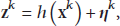
The residual vector is given by (12). The normalized norm of the residual vector for all five Ambiguity Trackers is shown in Figure 8. It can be seen how, on average, the correct Ambiguity Tracker AT1 presents a lower residual error in the range below.

Figure 8

A comparison of the normalized residuals of five different Ambiguity Trackers during a 200 s run. The Ambiguity Tracker following the correct integer ambiguity vector (AT1) has generally the lowest normalized residual.

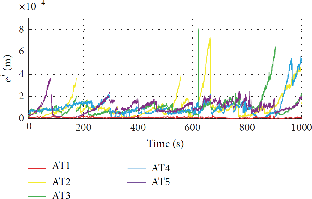
Both parameters are used to weight each of the five Ambiguity Tracker hypotheses. Figure 9 shows the weight of each of the Ambiguity Trackers. As explained in Section 3, the weight is a value between $\mathrm{0}$ and $\mathrm{1}$ , and the sum of all weights amounts to one. All weights are initialized to the same value and quickly AT1, the Ambiguity Tracker we know that is the correct one from the previous experiment, gets a higher weight. Each time the weight of an Ambiguity Tracker falls below a certain threshold the Ambiguity Tracker is eliminated and a new one is initialized with some weight that is “stolen” from the other Ambiguity Trackers.

Figure 9

An evaluation of the weight of five different Ambiguity Trackers during a 200 s run. The Ambiguity Tracker following the correct integer ambiguity vector (AT1) quickly gets more weight than the others.

This experiment demonstrates that weighting according to the normalized residual and the number of tracked satellites makes it possible to successfully find the correct Ambiguity Tracker.

5.4. Baseline Tracking Filter

In this test, the performance of the Baseline Tracking Filter presented in Section 4 is evaluated. The strategy of this Kalman filter is to give more weight to those Ambiguity Trackers whose baseline coordinates are closer to this predicted baseline. This weighting parameter will help to identify faster the correct solution in case that the correct solution is lost.

In this case, this test run lasts almost 9 minutes, and it is divided into two parts. The first part is the same stretch used in the previous two experiments. The second part begins with both vehicles at a standstill at approximately 5.7 m distance; then they start accelerating and finally they stop again at the end of the stretch.

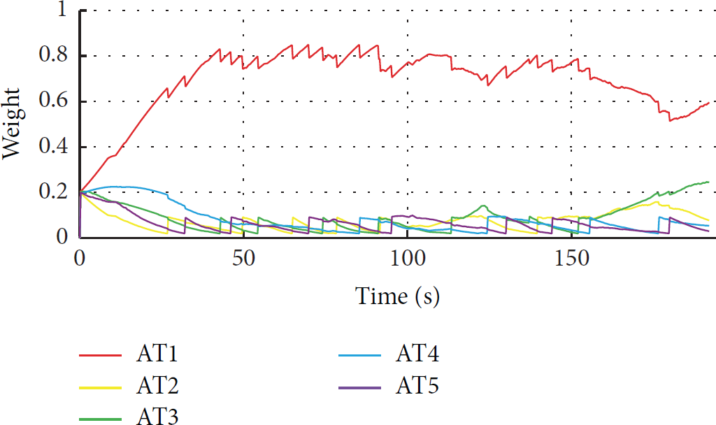
In the second part of this test run, the Ambiguity Tracker method loses the track of the correct solution mainly due to obstacles near the road, which causes numerous cycle slips and many satellite blockages. One example is shown in Figure 10, where the baseline lengths of the five Ambiguity Trackers are compared with the laser scanner. It can be seen how all five Ambiguity Trackers lose the track of their baseline solutions in second 357. Until then, the correct solution is tracked by AT5. After the outage, the five Ambiguity Trackers are reinitialised. Without the Baseline Tracking Filter (not shown here) none of the Ambiguity Trackers is able to find the correct solution, all of them being initialized and discarded over and over again. However, by incorporating the Baseline Tracking Filter and predicting the baseline using the speed and the heading of each vehicle, it is possible to weight the reinitialized Ambiguity Trackers with the predicted solution and eventually find the correct solution as shown in Figure 10. AT1 is able to recover the correct solution.

Figure 10

A comparison of the baseline length of five different Ambiguity Trackers when an outage occurs. After the outage, the correct integer ambiguity vector is recovered by the Ambiguity Tracker AT1.

The weight of each Ambiguity Tracker along the entire test run is shown in Figure 11. It can be seen how after the outage in second 357 AT1 quickly gets more weight than the others. Therefore, we can conclude that the Baseline Tracking Filter improves the global performance of the Multiple Ambiguity Hypotheses method.

Figure 11

An evaluation of the weight of five different Ambiguity Trackers during a 527 s run using the Baseline Tracking Filter. The system correctly recovers after carrier phase loss of lock and the correct Ambiguity Trackers (AT1, AT5, and AT1) quickly get more weight than the others.

An increased occurrence of signal obstructions and cycle slips, for instance, while driving in an urban-like environment, will limit the applicability of the presented method. To approach these scenarios a sensor fusion solution using on-board sensors, such as steering wheel angle sensor and wheel tick odometers, could stabilize the baseline prediction for longer periods of time. This, however, falls out of the scope of the current paper and is left as future work.

5.5. Computational Resources

The multiple Ambiguity Tracker algorithm has been run on an Intel i7 64-bit processor at 2.10 GHz. A recorded test run of 527 s has been processed and the computation time has been measured. Figure 12 shows the computation time in dependance of the number of initialized Ambiguity Trackers for both, processing measurements at 4 Hz and 10 Hz. The dashed red line represents the real-time processing limit, above which the computation time exceeds the real time. Up to 29 Ambiguity Trackers can be run in real time at 4 Hz and up to 16 at 10 Hz.

Figure 12

Computational complexity study with regard to the number of initialized Ambiguity Trackers. Two GPS receivers with different measurement update rates have been analyzed.

The previous analysis is performed on a test run in a benign environment. The computation time is, however, partly correlated to the environment. The more frequently the cycle slips occur, the more the satellites are placed in quarantine and need to be checked for being healthy again. Consequently, a slightly lower number of Ambiguity Trackers are expected to be run in more challenging signal conditions.

Regarding the memory requirements, each Ambiguity Tracker only stores the current integer ambiguity, the satellite number of tracked satellites and satellites in quarantine, the baseline, baseline velocity, and baseline acceleration.

6. Conclusion

In this paper we proposed a new method to determine the relative position of two vehicles using a cooperative approach exchanging GNSS raw measurements. The Ambiguity Tracker solves and tracks the carrier phase double difference integer ambiguity vector and computes a precise relative position between vehicles. The Ambiguity Tracker is based on single-epoch LAMBDA method to find the most likely integer ambiguity vector and be robust against cycle slips. The approach is designed to be used for low-cost single-frequency receivers that are already integrated in modern vehicles.

We have demonstrated how running multiple Ambiguity Trackers in parallel and correctly weighting them make it possible to find the correct integer ambiguity. A Kalman filter tracking the baseline improves the method in situations of momentary blockage. The proposed method has been tested in an open-sky rural environment with two vehicles driving behind each other. It has been demonstrated that the proposed approach is able to track with subcentimeter accuracy the baseline using Ublox LEA 4T GPS receivers. This method is designed to run in real time and is able to track up to 30 integer ambiguities on a modern notebook.

Future lines of work include the integration of the proposed approach with on-board sensors to better predict the baseline over time and with other relative positioning information sources, as, for instance, a radar or a laser scanner sensor, in order to weight the Ambiguity Trackers and be able to find the correct solution more quickly.