Feature Extraction in Densely Sensed Environments: Extensions to Multiple Broadcast Domains

Abstract

The vision of the Internet of Things (IoT) includes large and dense deployment of interconnected smart sensing and monitoring devices. This vast deployment necessitates collection and processing of large volume of measurement data. However, collecting all the measured data from individual devices on such a scale may be impractical and time-consuming. Moreover, processing these measurements requires complex algorithms to extract useful information. Thus, it becomes imperative to devise distributed information processing mechanisms that identify application-specific features in a timely manner and with low overhead. In this paper, we present a feature extraction mechanism for dense networks that takes advantage of dominance-based medium access control (MAC) protocols to (i) efficiently obtain global extrema of the sensed quantities, (ii) extract local extrema, and (iii) detect the boundaries of events, by using simple transforms that nodes employ on their local data. We extend our results for a large dense network with multiple broadcast domains (MBD). We discuss and compare two approaches for addressing the challenges with MBD and we show through extensive evaluations that our proposed distributed MBD approach is fast and efficient at retrieving the most valuable measurements, independent of the number sensor nodes in the network.

1. Introduction

Several technological advancements in hardware design enable IoT application scenarios with very dense deployments of sensor nodes. Researchers are designing tiny radio-on-a-chip communication devices with processing and communication capabilities. These low-power wireless devices can also be powered from the energy scavenged from ambient radio waves [1]. Several market studies project that trillions of things will soon be connected to the Internet [2]. In a large-scale dense network, the amount of collected data will therefore be enormous and it becomes necessary to extract only the information that is relevant to further processing [3]. For example, in some cases, it maybe required to alert the occurrence of certain features in a timely manner.

In this work, we tackle the problem of feature extraction in a dense IoT application. (An earlier version of this work was published in the proceeding of DCOSS 2014, DOI: 10.1109/DCOSS.2014.29. This work considered a single broadcast domain (SBD), where all nodes are located within the same transmission range.) We define feature extraction as the process of determining certain features such as peaks, boundaries, and shapes in the distribution of a physical quantity.

While feature extraction may not be an issue for a low density network (e.g., tens of sensor nodes), it is still a challenging problem for a high density network. In applications requiring measurements with a high spatial granularity, covering even a small area (e.g., one square meter) may require hundreds to thousands of sensor nodes. Some examples of densely deployed sensing nodes, where features of one or more physical quantities need to be monitored frequently, are sleep monitoring for health-care applications [4], smart surfaces for aviation systems [5], and fruit monitoring in agriculture industries [6].

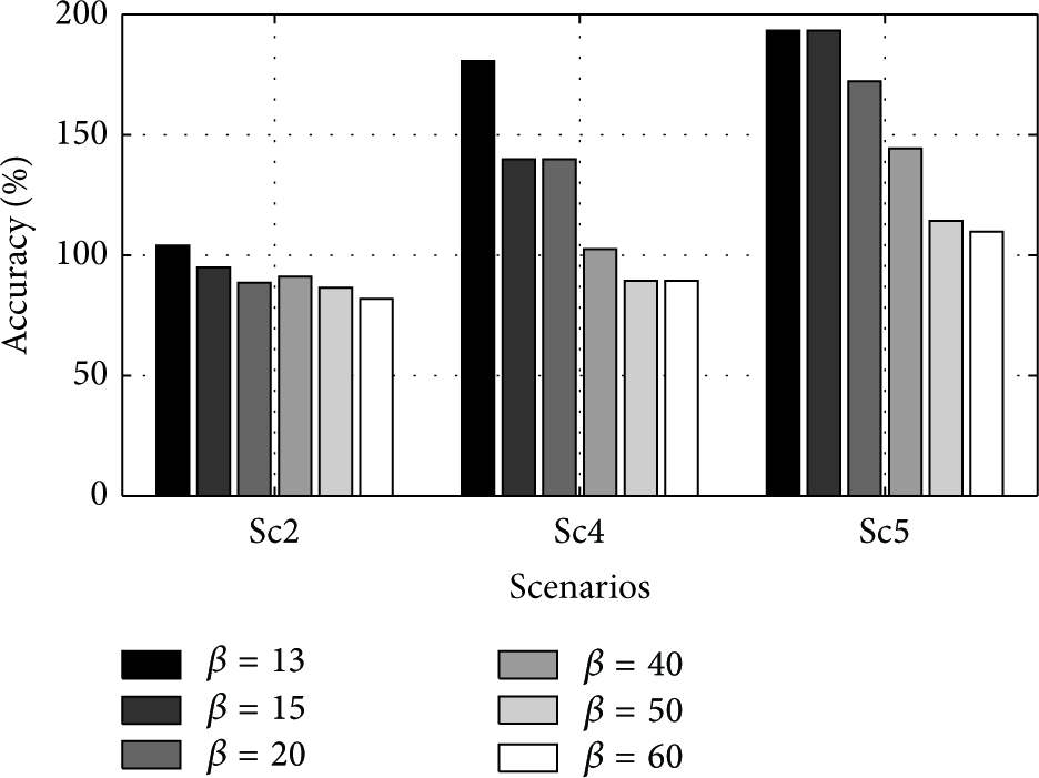
Figure 1 presents an example distribution of the measurements of a physical quantity (e.g., temperature or pressure values). As shown, the distribution has three distinct regions of activity that require detection and evaluation. Such a dense sensor network for measuring a physical quantity, called a field, would involve deploying one sensor node to measure each data point in the distribution. The regions of activity, called active regions, are those where the values measured by sensor nodes are of interest.

Figure 1

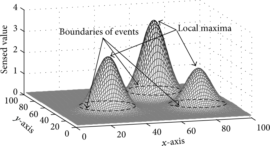
An example of a 2D physical quantity field with 10,000 sensor nodes. Each data point corresponds to a value sensed by an individual node.

One naive way to identify active regions would be to collect readings from all sensor nodes and process them centrally. This is usually inefficient since typical channel access techniques do not scale well with an increase in number of nodes. It is therefore advantageous to devise techniques that identify active regions irrespective of the density of the network.

Computing even simple aggregate quantities such as extrema (minimum or maximum) is not trivial for a dense network as it may require collecting data, in the worst case, from all nodes [7] (even if some sort of spatial subsampling is employed [8]). Dominance-based or binary-countdown MAC protocols help in finding the minimum value in constant time [9–11], provided that all nodes reside in a single broadcast domain (SBD). Furthermore, finding peaks and their boundaries in a distributed network, where each data point is measured by individual sensor nodes, is computationally expensive, is time-consuming, and typically does not even scale linearly with respect to network size.

In [3], we first proposed a set of feature extraction techniques for an SBD and established that finding the local extrema is a challenge in an SBD even after the global maximum is known. Once the global maximum is identified in constant time, we proposed a few transforms that nodes employ on local data, which helps in identifying other peaks (local maxima) and their boundaries in the spread of the physical quantity being measured. Our proposed transforms, referred to as augmenting functions, allow the identification of local extrema in constant time. We showed that, instead of collecting all data as in the naive case, these augmenting functions retrieve the most valuable sensor nodes’ measurements that result in fewer number of measurements being collected.

In this paper, we present the design, implementation, and evaluation of a set of distributed algorithms to extract certain features of a physical quantity in a dense sensor network. We enhance our preliminary work published at [3] with the following new contributions:

• (i)

We propose a new distributed algorithm (dubbed ripple-based) to extend the process of obtaining global extrema in an MBD dense network. Since finding global extrema is the main building block in the proposed augmenting functions, this extension enables the applicability of these functions for MBD networks.

(ii)

We modify an existing clustering approach [12] to obtain the global extrema for MBD networks and compare the novel ripple-based approach with the classical cluster-based approach and evaluate their efficiencies.

(iii)

We design a simulation model to analyze the impact of relevant network parameters (e.g., communication range in wireless medium) on the functioning of the ripple-based approach.

This paper is organized as follows. An outline of other works related to our approach is given in Section 2 after a brief introduction on the dominance-based approach. The architecture and the system description based on an aggregate quantity function are provided in Section 3. Afterwards, we introduce various augmenting functions that are used to transform the sensor value such that local extrema or boundaries in various directions become the global extremum. In Section 5, a brief explanation of the clustering approach is given, followed by a novel approach, called ripple-based, to obtain the global extrema in an MBD network. This approach is fully distributed and exploits concurrent transmissions of dominance-based protocols. In Section 6, the evaluation of proposed augmenting functions is given together with a comprehensive comparison on the cluster-based and the ripple-based approaches for MBD networks.

2. Background and Related Work

Detection of events in sensor networks is a major application domain and a very broad topic. There are different approaches to address the problem of boundary detection in dense sensor networks. To the best of our knowledge, this is the first boundary detection technique that utilizes dominance-based MAC protocols. To this end, first we provide a detailed explanation of this MAC paradigm and explain how to compute an aggregate value (e.g., globalMIN) utilizing the dominance-based MAC protocol, followed by an outline of related work.

2.1. Dominance-Based Approach

This work is inspired from dominance-based or binary-countdown protocols [9] implemented for wired networks in the widely used CAN bus [10] as well as its wireless version, called WiDom [11]. The major reason for using a dominance-based MAC protocol is its scalability and constant time-complexity even for very dense networks. In this work, we focus on time-complexity and we do not enrich our dominance-based MAC protocol with sleep states or other energy-saving mechanisms; thus, the current state of the protocol is ready to be used in critical applications where energy issues are not the main focus of the scenarios.

In dominance-based MAC protocols, each node is associated with a priority value that is used to resolve the medium contention. All nodes “simultaneously” start a conflict resolution phase which we refer to as tournament (depicted in Figure 2), by transmitting synchronously their priority values bit-by-bit, starting with the most significant one, while simultaneously monitoring the medium. The medium must be devised in such a way that nodes will only detect a “1” value if no other nodes are transmitting a “0.” Otherwise, every node detects a “0” value regardless of what the node itself is sending. For this reason, a “0” is said to be a dominant bit, while a “1” is said to be a recessive bit. Therefore, low numbers in the priority field of a message represent high priorities. If a node contends with a recessive bit but hears a dominant bit, then it will refrain from transmitting any further bits and will proceed only monitoring the medium. Since the medium acts as a logicalAND operator, the node with the smallest priority value (winner) gains access to the medium.

Figure 2

Tournament in dominance/binary countdown protocols.

By using sensed physical quantities (like temperature or acceleration) as the message priority, various aggregate quantities can be obtained in dense networks. For instance, the minimum of sensed value (MIN) can be found by only one tournament (i.e., in constant time) [13].

In fact, simultaneous transmissions are a key to the time-efficiency of dominance-based MAC protocols. With carrier-sense or time-division based MAC protocols, computingMIN depends on the number of sensor nodes. Studies show that the computation ofMIN with standard IEEE 802.15.4 MAC linearly increases with the growth of network density (e.g., 80 ms for a 40-node network size) [7, 14]. Instead, the WiDom implementation [7] guarantees a constant time (10 ms) for calculatingMIN regardless of network density.

The process of findingMIN has been leveraged in the past to find an approximate interpolation and other aggregate quantities [7, 15]. Interpolated values are computed through an iterative process by integration of local information available at each sensor node (its own location information and measured value plus the location information and the measured value of the winner received after each tournament). Each sensor node computes the difference between its measurement and the corresponding computed interpolation value, known as the error value. This error is then used as the priority value in the conflict resolution phase. After a number of iterations (defined by user), an approximate interpolation of the physical quantity is obtained. However, instead of getting the complete interpolated image, in this work, we aim at detecting certain features of the physical quantity field by selecting a set of sensor nodes that hold the most valuable information.

2.2. Boundary Detection

The problem of boundary detection and determining the extent of an event in sensor networks has been investigated in [8, 16–19]. Chintalapudi and Govindan presented localized edge detection techniques based on statistics, image processing, and classification [16]. Nowak and Mitra described a method for hierarchical boundary estimation using recursive dyadic partitioning [8]. They developed an inverse proportionality relation between energy consumption and the mean-square error in boundary detection and showed that their method is near-optimal with respect to this fundamental trade-off. Another hierarchical boundary estimation is proposed in [19] where a contiguous 2D shape of an event is found with a threshold-based boundary detection.

Other schemes represent the boundary of an event or the signal landscape of a sensor network compactly using in-network aggregation [20–24]. Gandhi et al. studied the problem of monitoring the events of sensor networks using sparse sampling [21]. However, their algorithm requires the prior knowledge of the event geometry (e.g. circle, ellipse, or rectangle) for computational efficiency. Similar method has been explored in [23], which utilized a regression-based spatial estimation technique to determine discrete points on the boundary. Ham and Rodriguez present a distributed boundary detection based on in-network aggregation in which only sensor nodes that identify a boundary transmit their observation to the remote station [24]. To that end, they first applied a Delaunay triangulation to determine the neighbors of each node and then generate boundary segments between neighboring sensors. However, this algorithm cannot be known as a fully decentralized approach since the two steps mentioned above should be done centrally through a remote station.

There are also contour-based methods for deciding the type of an event [25, 26]. They consider energy-efficient techniques to construct and incrementally update a number of 2D contour maps in a sensor network. Another field of research involving detecting holes and topological features in a sensor network is presented in [27, 28]. In these approaches, local connectivity graphs are used to infer static features of an event and require the involvement of all the nodes in the network. By contrast, our approach is quite different from the above-mentioned techniques, as we exploit an underlying dominance-based MAC protocol for very sparse spatial sampling through a strategic selection of sensors.

3. System Model

We consider a sensor network where each sensor node has a unique identifier, i, and measures a particular physical quantity, $s_i$ , using a sensing unit. Each sensor node knows its 2D coordinates (x, y) in the plane of deployment. We assume that the feature extraction mechanism can be either carried out periodically as a part of a sense-process-actuate control-loop or sporadically initiated by an external controller, like a data sink or a master node.

The collection of all the sensor values across the total sensed area is referred to as a field (Figure 1). Each data point in the field corresponds to a true (or nonfaulty) sensor reading value, sensed by an individual sensor node at its physical location. The spatial granularity and the size of the field are directly correlated to the distribution of the nodes and their spread. We also define active region as a physical area populated by sensor nodes that sense some activity. The overarching goal of our approach is to find location, boundaries, and shape of an active region, which we referred to as features, in the physical environment. For illustrating our approach and its evaluation, we generated various sample fields by a summation of 2D Gaussian functions (explained in the appendix).

Function $\mathcal{M}(v_i)$ is defined as the process of findingMIN over values $v_i$ published by independent sensor nodes in a broadcast medium where $i\in \{\mathrm{1,2},\dots ,N\}$ and N is the number of sensor nodes in a broadcast domain. In fact, $\mathcal{M}(v_i)$ represents one execution of the tournament in an SBD (in Section 5.2 we discuss the details of function $\mathcal{M}$ for MBD, where several tournaments need to be run). We exploit the property of simultaneous transmissions in dominance-based protocols to devise this function. $v_i$ is the scaled value that each sensor node computes based on its measured value $s_i$ and the global maximum $s_{\max }$ measured in the field. Each application of $\mathcal{M}(v_i)$ is referred to as a round. After each round, all the other sensor nodes know the identifier and the location of the sensor node withMIN value. This sensor node is known as the winner of the round. We use $\widehat{i}$ to denote the identifier of the winner. Hence, function $\mathcal{M}$ can be formally represented as

$$\begin{array}{cc}& \left\{\widehat{v},\widehat{i},\widehat{x},\widehat{y}\right\}=\mathcal{M}\left(v_i\right)\forall i\in \left\{\mathrm{1,2},\dots ,N\right\},\end{array}$$

(1)

where $\widehat{x}$ and $\widehat{y}$ are the x and y coordinates of the sensor node with the global minimum value $\widehat{v}$ .

The choice of $v_i$ values used by an ith sensor node in the application of function $\mathcal{M}$ depends on the requirements of the application. It should be noted that a sensor node can only use its local information (such as identifier, sensor value, and physical location) and other global data available from previous iterations of $\mathcal{M}$ . For our goal of identifying various features, we augment (or transform) these input values in such a way that the globalMIN returned by $\mathcal{M}$ corresponds to one of the local minima or an edge of an active region.

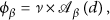
Function $\mathcal{M}$ can be applied to the value computed by ${\varphi }_i$ , which is a function of the sensor values and their location. The codomain of function ${\varphi }_i$ denotes the set of values it can take. We assume that the cardinality of the codomain of ${\varphi }_i$ is large enough that the probability of computing the same ${\varphi }_i$ by two sensor nodes is negligible and thus a unique sensor node $\widehat{i}$ is chosen. The time-complexity of $\mathcal{M}$ is proportional to the number of bits used to encode ${\varphi }_i$ and hence it is proportional to the logarithm of the cardinality of the codomain. However, as all sensor nodes transmit simultaneously in a dominance-based MAC protocol, the time required for the application of $\mathcal{M}$ over a network is independent of the number of sensor nodes. The abbreviations section summarizes the notations and symbols that we use in the following sections where we define a set of functions to extract different features of the field.

4. Feature Extraction Using Augmenting Functions

In this section, we describe in detail a set of augmenting functions that can extract an approximate but faithful representation of various features in the field by applying simple transforms on the sensor values.

We show that this process can be done with a limited number of broadcast messages or flooding in case of SBD or MBD, respectively.

4.1. ${\mathcal{A}}_{\beta }$ Distance Augmenting Function

As described earlier, a global maximum value in a sensor field can be easily found applying function $\mathcal{M}$ . However, finding the spread or boundaries of this peak (local maximum) is not trivial. If we modify the MAC protocol such that the sensor node with the global maximum does not participate in the next round, there is still a high chance that one of the adjacent sensor nodes to the peak will become the next local maximum. On the other hand, we might have to predefine a neighborhood range around the peak that should be excluded in the next cycle to make sure that another local maximum will be the new global maximum. In this case, choosing the size and shape of the neighborhood is also a challenge.

We demonstrate the process of finding an adjacent local minimum with a simple 1D Gaussian field example, shown in Figure 3. Using this example we show that, by utilizing the augmenting function over the input signal, the adjacent local minimum becomes the global minimum.

Figure 3

An example of augmented function ${\mathcal{A}}_{\beta }$ of the normalized input signal with various β in range of $[\mathrm{0.11,0.5})$ in 1D domain.

In this example, the field consists of three peaks and the highest peak (the global maximum) lies in the center. Finding the spread of this global maximum is not trivial as the global minimum point can be one of those sensor nodes near the borders of the field. It is important to suitably modify the process of identifying the extrema such that a local minimum adjacent to a peak (adjacent valley) can be found. For this purpose, we observe that an adjacent valley should have a low value and its distance from the peak should also be small. Hence, each value in the field is transformed (multiplied) with the distance from the peak. With this transformation, the points located farther from the peak are associated with higher values (compared with its sensed value) and only points with lowest sensed value and smallest distance from the peak can become the global minimum in the augmented field. It is possible that this global minimum is a point in an adjacent valley. The boundary of this peak is found with just two rounds of executing $\mathcal{M}$ function: (i) finding the global maximum in the original field and (ii) identifying the global minimum in the augmented field.

For 2D Gaussian fields, the 1D approach described above can be directly applied. Different active regions of the field are found by excluding the sensor nodes lying inside the identified active region from participating in the next rounds. The process of finding active regions is shown in Algorithm 1. Initially, function $\mathcal{M}$ is used to find the global maximum $s_{\max }$ , and then a circular area around the identified peak is filtered out. The radius of this filtering circle is set as the distance of an adjacent valley from the peak. The value and the location of the adjacent valley ( $S_{\text{adj-valley}}$ and $d_{\text{adj-valley}}$ ) are found by one application of $\mathcal{M}$ function (line 9 in Algorithm 1).

Algorithm 1: Distance augmenting function ${\mathcal{A}}_{\beta }$ , executed on each sensor node $n_i$ .

$(\mathit{1}$ ) begin

( $\mathit{2}$ )   $Silent\leftarrow \mathrm{0}$ ;

( $\mathit{3}$ )   $s_{\max }\leftarrow \mathcal{M}(-{\varphi }_s)$ ; // find global MAX

( $\mathit{4}$ )   ${\pi }_s\leftarrow$ a fraction of $s_{\max }$ ; // termination condition setting

( $\mathit{5}$ )  while $s_{\text{new-peak}}>{\pi }_s$ do

( $\mathit{6}$ )   if $Silent\ne \mathrm{1}$ then // not filtered out

( $\mathit{7}$ )     $s_{\text{new-peak}}\leftarrow \mathcal{M}(-{\varphi }_s)$ ; // find the new peak

( $\mathit{8}$ )    Compute ϕ based on (2);

( $\mathit{9}$ )     $〈s_{\text{adj-valley}},d_{\text{adj-valley}}〉\leftarrow \mathcal{M}({\varphi }_{\beta })$ ;

( $\mathit{10}$ )    $R_f\leftarrow d_{\text{adj-valley}}$ ;

( $\mathit{11}$ )    $d_i\leftarrow$ distance between new-peak and node $n_i$ ;

( $\mathit{12}$ )   if $d_i<R_f$ then

( $\mathit{13}$ )     $Silent\leftarrow \mathrm{1}$ ;

Each sensor node uses function ${\varphi }_{\beta }$ as an input to $\mathcal{M}$ . Function ${\varphi }_{\beta }$ takes into account two properties of the field, sensed value s and sensor's proximity to the peak d, and is defined as follows:

$$\begin{array}{cc}& {\varphi }_{\beta }=\nu \times {\mathcal{A}}_{\beta }\left(d\right),\end{array}$$

(2)

where ν is the scaled value and is defined as

$$\begin{array}{cc}& \nu =\frac{\mathrm{1}+s}{\mathrm{1}+s_{\max }}\end{array}$$

(3)

and $s_{\max }$ is the value of the global maximum, found at the beginning of the algorithm. ${\mathcal{A}}_{\beta }(d)$ is the augmenting function, which is formulated as follows:

$$\begin{array}{cc}& {\mathcal{A}}_{\beta }\left(d\right)=e^{\beta {\left(d/d_{\max }\right)}^{\mathrm{2}}},\end{array}$$

(4)

where $d_{\max }$ is the diameter of the monitored area and it is used to normalize the distance from the peak and β is a parameter to control the impact of distance on the augmented field with respect to the scaled value ν. To ensure that the winning sensor node is located at the adjacent local minimum of the field, the priority function ${\varphi }_{\beta }$ is computed so that the distance is exponentially penalized.

Finally, by finding the global minimum over ${\varphi }_{\beta }$ values at all the sensor nodes, we can find a point that lies in the adjacent valley with high probability. The distance between the adjacent valley point and the peak determines the filtering radius, $R_f$ (line 10 in Algorithm 1). Sensor nodes that are located within the filtering circle refrain from participating in the next iterations. Repeating this procedure helps in finding all the peaks in the region. The algorithm stops when the value of new peak ( $s_{\text{new-peak}}$ ) is lower than a certain user defined threshold ${\pi }_s$ , which is a fraction of the global maximum. By finding the peaks and their spread, this approach helps in identifying the location and the number of circular active regions in a field.

4.2. ${\mathcal{A}}_{\gamma }$ Vector Augmenting Function

Our second augmenting function is used for cases where we are interested in finding a boundary around the whole active region. This approach can be used for a range of applications such as crowd monitoring for smart cities or sleep monitoring for health-care. In this approach, if we assign larger values of ϕ to sensor nodes that lie on the boundary of an active region, then the result of applying the $\mathcal{M}$ function over the negation of ϕ value corresponds to the boundary of the active region. This is implemented by augmenting the sensor values with a function that grows in a particular direction.

The vector augmenting function, ${\mathcal{A}}_{\gamma }$ , is designed to work with binary fields, where the input signal is not smoothly distributed, and two neighboring sensor nodes may have very close or very different measurements. By applying ${\mathcal{A}}_{\gamma }$ , each sensor node multiplies its measurement with a vector $\overrightarrow{u}$ . The rationale behind using a direction is to find sensor nodes that sense a high value and are located as far as possible in the direction given by $\overrightarrow{u}$ , which corresponds to the edge of an active region in that direction. To compute function ϕ, sensor nodes transform their locations with a direction as

$$\begin{array}{cc}& {\varphi }_{\gamma }=v_p\times {\mathcal{A}}_{\gamma }\left(x,y,\theta \right),\end{array}$$

(5)

where $v_p$ is a participation value which is either $\mathrm{0}$ or $\mathrm{1}$ depending on the sensed value being below or above a threshold. Sensor nodes with $v_p=\mathrm{1}$ are part of the active region. The augmenting function is defined as

$$\begin{array}{cc}& {\mathcal{A}}_{\gamma }\left(x,y,\theta \right)=e^{\gamma \left(x·\cos \left(\theta \right)+y·\sin \left(\theta \right)\right)},\end{array}$$

(6)

where x and y are the coordinates of the sensor location and θ is the direction given by vector $\overrightarrow{u}$ .

By using ${\mathcal{A}}_{\gamma }$ , the value is “projected” in a direction given by the vector $\overrightarrow{u}$ . The sensor node that has the largest value has a high probability of being located on the border of an active region in the direction of $\overrightarrow{u}$ .

The working of this approach is outlined in Algorithm 2. The algorithm explores the region by choosing random directions defined in a set $\{\overline{v_{\theta }}\}$ . We assume that the seed for generating these pseudorandom directions is generated by the initiator of the boundary detection process (thus, all the sensor nodes will use the same $\{\overline{v_{\theta }}\}$ in each iteration). Repeating this procedure in different directions makes it possible to find the boundary of an active region by computing the convex hull of the collected locations.

Algorithm 2: Vector augmenting function ${\mathcal{A}}_{\gamma }$ , executed on each sensor node $n_i$ .

$(\mathit{1}$ ) begin

( $\mathit{2}$ )   $s_{\max }\leftarrow \mathcal{M}(-{\varphi }_s)$ ; // find global MAX

( $\mathit{3}$ )   ${\pi }_s\leftarrow$ a fraction of $s_{\max }$ ; // termination condition setting

( $\mathit{4}$ )   $\{f_{\theta }\}\leftarrow \mathrm{⌀}$ ; // filtered direction set

( $\mathit{5}$ )  if $s<{\pi }_s$ then

( $\mathit{6}$ )    $v_p\leftarrow \mathrm{1}$ ;

( $\mathit{7}$ )  else

( $\mathit{8}$ )    $v_p\leftarrow \mathrm{0}$ ;

( $\mathit{9}$ )   $\{\stackrel{-}{v_{\theta }}\}\leftarrow$ a set of θ directions;

( $\mathit{10}$ ) foreach $\theta \in \{\stackrel{-}{v_{\theta }}\}$ do

( $\mathit{11}$ )   if $\theta \notin \{f_{\theta }\}$ then

( $\mathit{12}$ )    Compute ${\varphi }_{\gamma }$ based on (5);

( $\mathit{13}$ )     $〈s_{\text{edge}},(x,y{)}_{\text{edge}},{\theta }_{\text{edge}}〉\leftarrow \mathcal{M}(-{\varphi }_{\gamma })$ ;

( $\mathit{14}$ )    if $(x,y{)}_{\text{edge}}$  was found with other direction, ${\theta }_x$

     then

( $\mathit{15}$ )       $$\left\{f_{\theta }\right\}⟵\left\{f_{\theta }\right\}\cup \stackrel{⌢}{{\theta }_x\theta }+\mathrm{2}ϵ$$ ;

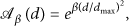
If two angles lead to the same point, it means that any angle over the arc confined by these two angles would result in that point. Thus, this arc can be filtered out from further investigation. Figure 4 shows an example where two angles of ${\theta }_{\mathrm{1}}={\mathrm{31}}^{\circ }$ and ${\theta }_{\mathrm{2}}={\mathrm{89}}^{\circ }$ lead to find the same location $P_{\mathrm{2}}$ . In this case, there is no need to examine more directions in the region of ${\mathrm{31}}^{\circ }\le \theta \le {\mathrm{89}}^{\circ }$ . To further limit the redundant directions from the set $\{\overline{v_{\theta }}\}$ , we introduce a marginal extension factor, ϵ. Doing so, the redundant arc will be further confined by ${\theta }_i\pm ϵ$ . We discuss the impact of ϵ in Section 6.

Figure 4

An example of boundary detection for a hexagonal-shape event.

More iterations of the algorithm leads to more accurate boundaries, but at the cost of more resource consumption. We show in Section 6 that, with the above filtering strategy, we are able to reduce the number of dominance rounds, while still building a good description of the active region. The worst case for our algorithm happens when the event boundary looks like a perfect circle where new directions will always give new points (considering a very dense deployment of sensors and a marginal extension of $ϵ={\mathrm{1}}^{\circ }$ , in this case, up to $\mathrm{359}$ individual readings will be collected). However, the results show that the number of readings is usually much less in practice.

4.3. ${\mathcal{A}}_{\delta }$ Joint Augmenting Function

As described earlier, the distance augmenting function ${\mathcal{A}}_{\beta }$ identifies circular active regions. For complex fields, ${\mathcal{A}}_{\beta }$ may need several circular active regions to cover a noncircular shape. On the other hand, vector augmenting function ${\mathcal{A}}_{\gamma }$ only provides a convex hull of all the active regions. So a field with several isolated active regions is identified as one large shape, which may not provide enough insights regarding the structure of the active regions.

To find the boundary of an active region with noncircular distribution, we devised a new augmenting function, ${\mathcal{A}}_{\delta }$ , that is a composition of ${\mathcal{A}}_{\beta }$ and ${\mathcal{A}}_{\gamma }$ . By applying ${\mathcal{A}}_{\delta }$ sensor nodes that identified with $\mathcal{M}$ function should have the following properties: (i) lying close to the peak and (ii) being located on the edge of the local boundary in a given direction, the value used by each sensor node is then defined as follows:

$$\begin{array}{cc}& {\varphi }_{\delta }={\mathcal{A}}_{\delta }\times \frac{{\mathcal{A}}_{\beta }\left(d\right)}{{\mathcal{A}}_{\gamma }\left(x,y,\theta \right)},\end{array}$$

(7)

where ${\mathcal{A}}_{\delta }$ is given by

$$\begin{array}{cc}& {\mathcal{A}}_{\delta }={\nu }^{-\delta }.\end{array}$$

(8)

${\mathcal{A}}_{\delta }$ is an inverse polynomial of degree δ of the scaled sensed value, ν, and δ is a parameter to guarantee that the low values lying far away from a peak bring a stronger contribution to the ϕ values. As a consequence, for a given value of θ, the point that has the minimum value of ${\varphi }_{\delta }$ is more likely to lie on the boundary in the θ direction. We sweep the area around a peak with different values of θ. In our evaluation, for θ, we used equal intervals of $\pi /\mathrm{4}(\theta \in \{\mathrm{0},\pi /\mathrm{4},\dots ,\mathrm{2}\pi \})$   (smaller intervals will result in better accuracy of boundary at the cost of higher number of broadcast messages.). Thus, after finding a new peak, the locations of the nearest adjacent valleys in eight directions are found and the convex hull of all these readings represents the area around that active region. This enables us to find complex geometric shapes according to the shape of active regions instead of only circles, as shown with an example in Figure 5.

Figure 5

An example of boundary detection around the peaks with nonuniform distribution.

5. Computing Global Extrema in MBD Networks

In this section, we address the challenge of computingMIN in a dense network, where nodes are not necessarily confined in an SBD. We consider two different approaches to extend the functionality of $\mathcal{M}$ function for MBD dense networks: (i) clustering the network into several SBDs as proposed in [12] and (ii) a novel approach using concurrent transmissions by taking advantage of the dominance-based protocol.

5.1. Cluster-Based Approach

In the clustering approach, proposed in [12], a topology discovery algorithm is first executed to partition the network such that all nodes in each partition are in the same broadcast domain (Setup phase). Then, at runtime, nodes within the same cluster find the minimum sensor reading and communicate these values to their cluster leaders. The cluster leaders form a collection tree with root at the leader node where the query for computingMIN was initiated.

The high-level pseudocode of the cluster-based approach is given in Algorithm 3. A minimum virtual dominating set (MVDS), as introduced in [29], has been considered during the setup phase. With MVDS, it is possible to divide the network into several clusters where the nodes in each cluster form an SBD. The cluster leaders (known as black-nodes in MVDS) are responsible for collectingMIN in each cluster and forwarding it to the leader node through a collection tree graph known as black-node tree (B). The virtual range is used to guarantee that all nodes in a cluster are located in the same broadcast domain. In fact, the MVDS is a distributed algorithm with two main phases. In the propagation phase, it forms the clusters; and, in the response phase, the topology information is delivered to the leader node (the node initiating the aggregation query). Figure 6(a) shows an example of cluster construction using MVDS.

Algorithm 3: Cluster-based approach.

( $\mathit{1}$ ) begin

( $\mathit{2}$ )  runMVDS( $R_{\mathrm{co}},r$ ) [29] to partition the network (setup phase); // execute on each sensor node  $n_i$

( $\mathit{3}$ )  construct cluster interfering graph $G_i(V,E)$ and black-node tree B (response phase); // execute on leader node

( $\mathit{4}$ )   $\mathrm{\Delta }\leftarrow$   timeslot-assignment(G); // executed on leader node

( $\mathit{5}$ )  for $i=\mathrm{1}$ toΔdo

( $\mathit{6}$ )   execute one dominance round according to assigned timeslot; // execute on nodes in each active cluster

( $\mathit{7}$ )  collect data from black-node tree B; // execute on leader node

( $\mathit{8}$ )  disseminate global MIN to the network; // execute on leader node

Figure 6

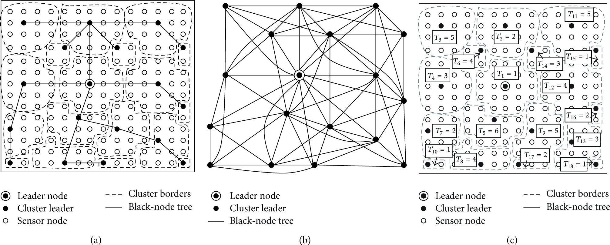
Cluster-based approach: (a) cluster formation and black-node tree (B) construction. $R_{\mathrm{co}}=\mathrm{5}$ and we assume that $r=R_{\mathrm{co}}/\mathrm{2}$ . With the given virtual range r, 18 clusters are constructed; (b) cluster interfering graph $G_i$ (with $d=\mathrm{14}$ ). This graph is used by the leader node to compute the activation time slot for each cluster. Two clusters are assumed to be interfering if the distance between the cluster leaders is less than $\mathrm{3}\times r$ ; (c) time slot assignments (the chromatic number for the interfering graph is 6).

The leader node uses this topology information to schedule the activation time of each cluster to avoid any collision between neighboring nodes that reside in different clusters. To make this approach more efficient, we utilize a heuristic that was proposed for the register interfering graph (RIG) problem [30] to find the chromatic number Δ for concurrent active clusters. However, unlike the RIG problem, in our case the number of available colors is not known in advance. This is the number of registers in RIG problem, k.

Functiontime slot-assignment(G) is performed by the leader node to find the value of Δ as shown in Algorithm 4. From basic graph theory it is known that, for an n-node graph $G(V_n,E)$ , if the maximum degree of nodes in the graph is d, then it is possible to color the graph with $d+\mathrm{1}$ different colors [31]. In our modified heuristic, the leader node initiates the process of finding Δ by setting k to $⌈\left(d+\mathrm{1}\right)/\mathrm{2}⌉$ and then restricts the search area $[k_{\min },k_{\max }]$ . If the current k is able to color the graph (line 6 in Algorithm 4), the algorithm will add k into the set of possible chromatic numbers $\{C\}$ and updates $k_{\max }$ ; otherwise, it updates $k_{\min }$ . The algorithm terminates when the current k is larger than an element in the set $\{C\}$ . For the example given in Figure 6, with $d=\mathrm{14}$ the algorithm finds $\Delta =\mathrm{6}$ after four assignments of k.

Algorithm 4: Function timeslot-assignment( $G_i$ ), executed on the leader node.

$(\mathit{1}$ ) begin

( $\mathit{2}$ )   $\{C\}\leftarrow \mathrm{\varnothing }$ ; // possible chromatic numbers set

( $\mathit{3}$ )   $k_{\min }=\mathrm{0},k_{\max }=d+\mathrm{1},continue=\mathrm{1}$ , k- $colorable=\mathrm{0}$ ;

( $\mathit{4}$ )  while $continue==\mathrm{1}$ do

( $\mathit{5}$ )   $$k=⌈\frac{k_{\max }-k_{\min }}{\mathrm{2}}⌉+k_{\min }$$ ;

( $\mathit{6}$ )  ifk- $colorable==\mathrm{1}$ then // feasible to color the graph withknumber based on the heuristic in [30]

( $\mathit{7}$ )     $k_{\max }=k$ ;

( $\mathit{8}$ )    if $\{C\}\ne \mathrm{\varnothing }$ then

( $\mathit{9}$ )     foreach $k_i\in \{C\}$ do

( $\mathit{10}$ )      if $k\ge k_i$ then

( $\mathit{11}$ )        $continue=\mathrm{0}$ ;

( $\mathit{12}$ )    $\{C\}\leftarrow k$ ;

( $\mathit{13}$ )    else

( $\mathit{14}$ )    $k_{\min }=k$ ;

( $\mathit{15}$ )    $\mathrm{\Delta }\leftarrow \min \{C\}$ ;

5.2. Ripple-Based Approach

The ripple-based approach aims at eliminating the setup overhead in the cluster-based approach and mitigating the initialization cost by using a distributed algorithm to compute the global extrema. It uses the concurrent transmission property of the dominance-based protocol to find theMIN in an MBD network. The details of the ripple-based approach are provided in Algorithm 5. A good analogy for this algorithm is a ripple's propagation on a water surface and Figure 7 illustrates this approach with an example. Initially all sensor nodes are inactive ( $n_i$ -active $=\mathrm{0}$ ); that is, they do not participate in any tournament. The process is initiated by a sensor node broadcasting a query for computing the globalMIN. We assume that the query signal is a modulated wave which is used for both synchronization and starting a new tournament. Sensor nodes that receive this signal (i.e., in the initiator node's range) perform one tournament of dominance protocol to find aMIN value. Since only a subset of all nodes are participating in this stage, the resulting value is a localMIN. Immediately after finishing the first tournament, all sensor nodes, which had participated in the last tournament, initiate another tournament of the dominance protocol by sending a new query signal (with the newMIN value). This tournament in turn activates those sensor nodes, which are situated within the communication range, to change their status from idle to tournament state. This procedure continues until all nodes get activated.

Algorithm 5: Ripple-based approach, executed on each sensor node $n_i$ .

( $\mathit{1}$ ) begin

( $\mathit{2}$ )   $n_i\text{-}active=\mathrm{0}$ , $i=\mathrm{0}$ ;

( $\mathit{3}$ )  while $i\le \mathrm{2}\times ⌈D/R_{\mathrm{co}}⌉$ do

( $\mathit{4}$ )   i++;

( $\mathit{5}$ )   if $n_i\text{-}active==\mathrm{1}$ then broadcast the query signal;

( $\mathit{6}$ )   else if $n_i$  receives a query signal  then

( $\mathit{7}$ )     $n_i\text{-}active=\mathrm{1}$ ;

( $\mathit{8}$ )   execute one dominance round;

Figure 7

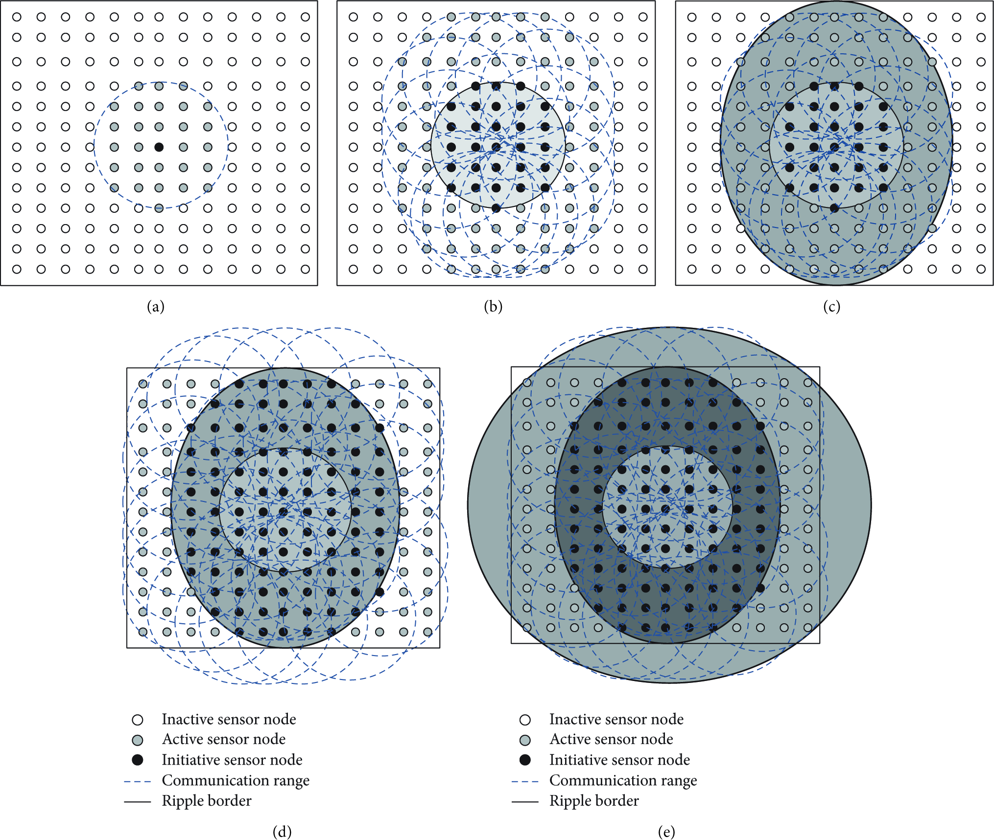
Ripple propagation throughout the network: (a) an initiator sensor node that signals start of a tournament. Sensor nodes within the communication range of this node then perform one tournament; (b) nodes participating in the previous tournament become initiator nodes in this round; (c) and (d) ripple moves toward the border of the network; and (e) all sensor nodes are activated.

To compute the globalMIN in an MBD network, the tournament needs to be run in worst case $\mathcal{N}=\mathrm{2}\times ⌈D/R_{\mathrm{co}}⌉$ times where D is the longest distance between two nodes belonging to the network (e.g., network diameter of the given square shape network) in number of hops and $R_{\mathrm{co}}$ is the communication range of sensor nodes. Note that this is an upper bound on the number of tournaments that needs to be performed till all nodes in the network become aware ofMIN. Figure 8 reveals the rationale behind this process with an example. This bounding event occurs when the sensor node with the lowest value and the initiator node are located at opposite ends of the network. Hence, it takes twice the length of $D/R_{\mathrm{co}}$ to assure that theMIN value is propagated to all sensor nodes.

Figure 8

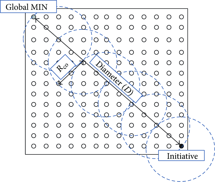
An example of the worst case scenario to determine the required number of tournaments ( $\mathcal{N}$ ). Assuming $D=\mathrm{12}\sqrt{\mathrm{2}}$ and $R_{\mathrm{co}}=\mathrm{2}\sqrt{\mathrm{2}}$ , the number of tournaments will be $\mathcal{N}=\mathrm{2}\times ⌈D/R_{\mathrm{co}}⌉=\mathrm{12}$ , that is, two times the number of circles depicted in this figure. In fact, it takes six tournaments to activate the node withMIN and another six tournaments to receive back the globalMIN by the initiative sensor node.

The $\mathcal{N}$ times execution of the tournament is corresponding to one application of $\mathcal{M}$ function or simply one round in MBD network. At the end of each round, the winner node broadcasts a packet which includes its location information and its identifier. This message is then flooded throughout the network, using the ripple-based approach, such that all nodes have the same knowledge about the properties of the winning node (note that, in SBD, this information is broadcastedonce by the winner).

Figure 9 shows an example of computingMIN in an MBD network, where the place of each node is represented by its measured value. In this example, we assume that the node located at the center of the network initiates the query for computingMIN (see Figure 9(a)). Sensor nodes in the communication range of the initiator execute one tournament. Since nodes that are located in the border of the communication range of the initiator are not reachable by each other, border sensor nodes find differentMIN values according to their location.

Figure 9

ComputeMIN in the MBD network. The evolution of determining theMIN value is shown in (a)–(f). The network diameter is $D=\mathrm{5}$ and communication range is $R_{\mathrm{co}}=\mathrm{2}$ . Pale numbers show inactive sensor nodes; dotted circles show the communication range in an SBD; the effective sensor nodes are shown in bold.

Figure 9(b) shows the result of findingMIN after execution of the first tournament. The two localMIN values are propagated in the first tournament (1 and 2). In the next iteration, all activated nodes perform the tournament and update theirMIN values (see Figure 9(c)). Finally, after five tournaments, the globalMIN is known throughout the network.

However, the multihop protocol described above can suffer from the hidden terminal problem. As dominance-based protocols allow nodes to listen toMIN value even from simultaneous receptions, hidden terminals in this case can cause a device in the middle to learn a spuriousMIN value.

To elaborate, consider three sensor nodes $N_{\mathrm{1}}$ , $N_{\mathrm{2}}$ , and $N_{\mathrm{3}}$ (with measured values 1, 2, and 3, resp.) as depicted in Figure 10. According to dominance-based protocols [9], during the tournament a sensor node transmits its measured value bit-by-bit. Upon knowing the existence of other nodes with a smaller measured value, it stops sending the rest of the bits. Now consider the scenario given in Figure 10(b). Node $N_{\mathrm{3}}$ loses the tournament after receiving the smallest value from node $N_{\mathrm{1}}$ . Since nodes $N_{\mathrm{1}}$ and $N_{\mathrm{2}}$ are not able to communicate directly, node $N_{\mathrm{2}}$ proceeds sending its last bit, which is $\mathrm{0}$ and node $N_{\mathrm{3}}$ mistakenly perceivesMIN in the network as $\mathrm{0}$ .

Figure 10

Example of hidden terminal problem during a tournament execution (we assume three priority bits): (a) network topology, (b) execution of tournament that leads to an error in node $N_{\mathrm{3}}$ , and (c) execution of tournament, including an extra time slot for bit retransmission.

To avoid this problem, we consider two slots for each bit transmission as proposed in [32]. The first slot is dedicated for the bit transmission itself and the second slot is dedicated for the retransmission of the bit detected during the first slot. If the current bit of a sensor node is dominant, there is no need to retransmit this bit for the second time, but if the bit is recessive and the sensor node detects a dominant bit during the transmission slot, it retransmits a dominant bit in the following retransmission slot (see Figure 10(c)). This bit-level redundancy solves the problem and leads to the correct perception ofMIN in the network. Obviously, it will increase the tournament duration.

6. Evaluation

We evaluated our proposed approaches in different simulated scenarios by considering the following three metrics.

Number of Rounds. A sensor node gets channel-access permit to broadcast a message in one round of execution of $\mathcal{M}$ function if its value is the global minimum. Hence, the number of rounds corresponds to the number of broadcast messages or flooding.

Accuracy. It represents the fraction of sensor nodes that declare themselves to be located in the active region(s) $N_{\det }$ to the number of sensor nodes that truly lie in the active region(s) $N_{\text{true}}$ :

$$\begin{array}{cc}& \text{Accuracy}=\frac{N_{\det }}{N_{\text{true}}}\times \mathrm{100}\left(\%\right).\end{array}$$

(9)

In cases where the detected area is larger than the actual active region, ( $N_{\det }>N_{\text{true}}$ ), accuracy is more than $\mathrm{100}\%$ , which signifies the overestimation of the active region.

Execution Time. It is the time needed to extract different features according to the proposed augmenting functions and is computed as

$$\begin{array}{cc}& \text{Exection\hspace{0.17em}\hspace{0.17em}Time}=\text{Number\hspace{0.17em}\hspace{0.17em}of\hspace{0.17em}\hspace{0.17em}Rounds}\times T_{\mathcal{M}},\end{array}$$

(10)

where $T_{\mathcal{M}}$ is the execution time of $\mathcal{M}$ function. In SBD networks, $T_{\mathcal{M}}$ is equal to one tournament duration. However, in MBD networks, $T_{\mathcal{M}}$ depends on the approach used for computing the global extrema (as discussed in Section 5).

We first show the process of computing $T_{\mathcal{M}}$ in MBD networks and then evaluate the feature extraction techniques for various scenarios.

6.1. Computing the Execution Time of $\mathcal{M}$ Function, $T_{\mathcal{M}}$

As stated earlier, the application of $\mathcal{M}$ function results in identifying the globalMIN over values of sensor nodes in a broadcast medium. We considered a network of size $\mathrm{100}\times \mathrm{100}$ sensor nodes in a shared medium. We change the communication range of sensor nodes $R_{\mathrm{co}}$ to study the performance of the new ripple-based and the classical cluster-based approaches in scenarios where the communication range of sensor nodes would divide the network into multiple broadcast domains. For the cluster-based approach, where clusters are built based on a virtual range, we set the range of virtual communication, r, to be always half of the actual communication range $R_{\mathrm{co}}$ of sensor nodes.

To have a precise computation of a tournament round, we consider the timeouts given in [33]. As illustrated in Figure 10, to solve the hidden terminal problem in the ripple-based approach, it is needed to send each bit twice during the tournament. Considering $\mathrm{110}$  μs as the length of one bit exchange [33], the tournament takes $\mathrm{110}\times n_{\text{prio}}+\eta$  μs for the cluster-based approach and $\mathrm{2}\times \mathrm{110}\times n_{\text{prio}}+\eta$  μs for the ripple-based approach where $n_{\text{prio}}$ is the number of priority bits and η is the time overhead imposed by the MAC protocol during the tournament (this extra time overhead is mainly due to synchronization and hardware shortcomings). For $n_{\text{prio}}=\mathrm{15}$ , the value of extra time overhead is $\eta =\mathrm{3099}$  μs [33]. Accordingly, the tournament takes $\mathrm{4749}$  μs and $\mathrm{6399}$  μs for cluster-based and ripple-based approaches, respectively.

Table 1 shows the number of referenced tournaments along with the time needed to find the global extremum in an MBD network. In this computation, we took into account the time needed to aggregate data in case of cluster-based approach, as well as the time required for flooding the local information of the winner in the ripple-based approach. However, in both cases we assume the best case scenario. For data aggregation through the black-node tree, we first compute the maximum degree d of the cluster interfering graph (see Figure 6(a)). To prevent any collision, it is considered that we need to have at least d time slots to collect data in the leader node. The duration of the time slot is considered to be the time needed to transmit a $\mathrm{128}$ byte-size packet. Assuming the IEEE 802.15.4-compliant MICAz's radio [34] with data rate of $\mathrm{250}$  Kb/s, the time-slot duration ( $T_s$ ) is then $\mathrm{4096}$  μs.

Table 1

Computation time of MIN value in cluster-based versus ripple-based approach.

Communication range	Cluster-based $(R_{\mathrm{co}},r)$		Ripple-based $(R_{\mathrm{co}})$
	Tnmta	Time (μs)	Tnmta	Time (μs)
$R_{\mathrm{co}}=\mathrm{14}$ , $r=\mathrm{7}$	$\mathrm{12}$	$\mathrm{159388}$	$\mathrm{8}$	$\mathrm{96248}$
$R_{\mathrm{co}}=\mathrm{20}$ , $r=\mathrm{10}$	$\mathrm{10}$	$\mathrm{137602}$	$\mathrm{5}$	$\mathrm{64763}$
$R_{\mathrm{co}}=\mathrm{28}$ , $r=\mathrm{14}$	$\mathrm{10}$	$\mathrm{141698}$	$\mathrm{4}$	$\mathrm{50172}$
$R_{\mathrm{co}}=\mathrm{34}$ , $r=\mathrm{17}$	$\mathrm{11}$	$\mathrm{150543}$	$\mathrm{3}$	$\mathrm{39677}$
$R_{\mathrm{co}}=\mathrm{40}$ , $r=\mathrm{20}$	$\mathrm{10}$	$\mathrm{137602}$	$\mathrm{3}$	$\mathrm{35581}$

${}^{\text{a}}$ Number of referenced tournaments.

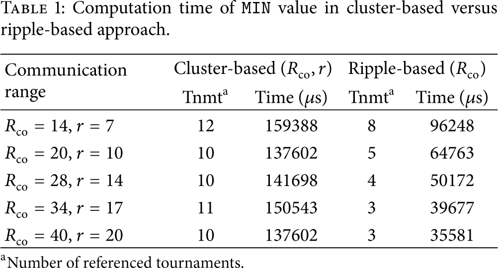
For the ripple-based approach, we compute the flooding time according to the theoretical lower latency bound given in [35]. Given that nodes transmit concurrently, the theoretical lower latency bound in a network with size h hops is $h·(T_s+T_d)$ . The number of hops is computed as $h=⌈D/R_{\mathrm{co}}⌉$ , where D is the network diameter and $R_{\mathrm{co}}$ is the communication range of sensor nodes. $T_d$ is the radio processing delay which is in the order of few microseconds and is determined by the radio; for simplicity, we ignore $T_d$ in our computation.

As expected, increasing the communication range results in faster computation ofMIN with the ripple-based approach. Also this method needs a smaller number of tournaments compared to the cluster-based approach. However, in the cluster-based approach, we do not observe the same continuous descending trend in the number of referenced tournaments. The reason is that the placement of the clusters plays an important role in the construction of the black-node tree and cluster interfering graph that affects the d value.

It should be mentioned that the given time for both approaches is slightly optimistic. In cluster-based approach, we do not consider the extra overhead imposed by the setup phase for cluster formation and similarly in ripple-based approach; we have used the lower bound of the flooding delay as in [35]. Note that, in the cluster-based approach, not all sensor nodes become aware ofMIN, while, in the ripple-based approach, which is a fully distributed algorithm, all nodes would knowMIN.

6.2. Identifying the Active Regions

We considered the same network settings as described in the previous subsection, with size of $\mathrm{100}\times \mathrm{100}$ sensor nodes. First, we show the performance of distance augmenting function to identify circular active regions. For evaluating our approach, we generated various scenarios with several active regions. The active regions may or may not overlap resulting in complex fields. The details of the scenarios are provided in Figure 24.

In each round of execution, after finding the global maximum, all the sensor nodes compute local values of ${\varphi }_{\beta }$ according to (2). Figure 11 illustrates the number of circular active regions with different termination rules for scenario sc1. Increasing the threshold level helps the algorithm to converge faster in smaller number of rounds, but at the cost of reduced accuracy.

Figure 11

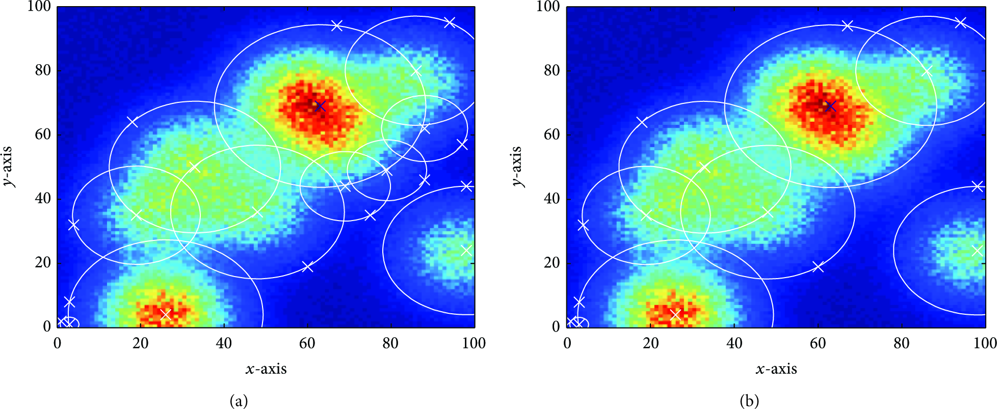
The effect of termination threshold, ${\pi }_s$ , on the detection of active regions. The algorithm terminates when a new detected peak is (a) $\mathrm{20}\%$ and (b) $\mathrm{30}\%$ of the global maximum value.

Figure 12 shows number of rounds and the corresponding obtained accuracy for different threshold values. We believe that the property of the field plays an important role in the number of required rounds and the accuracy of the detection. In some scenarios, increasing the termination threshold reduces the number of rounds as well as the overestimated area. This happens for scenarios sc1, sc3, and sc6, where the active regions can overlap. However, for scenarios sc2, sc4, and sc5, where either few active regions exist or the active regions are far apart, the number of rounds and accuracy remain almost the same for all termination conditions. The existence of isolated peaks in the field results in identifying all active regions by a fixed number of circular sections. The high value of overestimation in sc4 and sc5 is due to the steepness of the peak in the field. This steepness causes an overestimation in the filtering radius which in turn leads to much larger (squared) overestimation of the circle's area.

Figure 12

The number of rounds and the accuracy of active region estimation in different scenarios for various ${\pi }_s=\{\mathrm{10}\%,\mathrm{20}\%,\mathrm{30}\%\}$ of the global maximum.

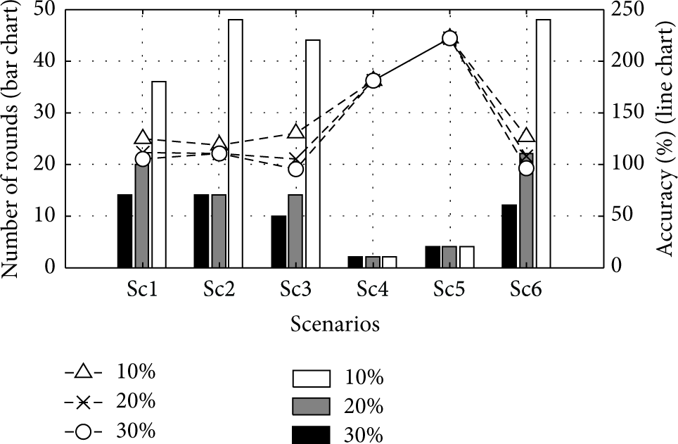
We found that the choice of the exponential coefficient β in our given heuristic (4) affects the overestimation of active regions. In fact, coefficient β impacts the relative weight of distance from the peak with respect to the value of the field at a given point. Choosing an optimal value of β is not possible without the prior knowledge of the field, but the order of β can be chosen based on the size of the field such that a proper trade-off between the sensor value at a given sensor node and its distance from the peak is maintained. Particularly, β should be chosen such that the impact of distance can be pronounced compared to the distance normalization ( $d_{\max }$ in (4)). For an area of $\mathrm{100}\times \mathrm{100}$ , we found that suitable values of β are in the order of $\mathrm{10}$ . Specific results on the accuracy for three scenarios sc2, sc4, and sc5 are shown in Figure 13. The main goal of this experiment was to investigate the level of overestimation given by ${\mathcal{A}}_{\beta }$ . It is observed that, for scenarios with isolated peaks, higher values of β improve the coverage estimation accuracy ( $\beta =\mathrm{40}$ for scenario sc4 and $\beta =\mathrm{60}$ for scenario sc5). But for scenarios where the spread of peaks overlap, the effect of changing β is less pronounced, as in the case of scenario sc2.

Figure 13

The effect of β on the accuracy.

Figure 14 shows the time it takes to detect the location of active regions by ${\mathcal{A}}_{\beta }$ . We examined the performance of cluster-based and ripple-based approaches for different communication ranges $R_{\mathrm{co}}=\{\mathrm{14,40}\}$ , which are the extreme ranges (shortest and longest) in Table 1. Interestingly, the execution time of ${\mathcal{A}}_{\beta }$ under ripple-based approach is at least $\mathrm{58}\%$ faster than that of the cluster-based approach. Increasing the communication range from $R_{\mathrm{co}}=\mathrm{14}$ to $R_{\mathrm{co}}=\mathrm{40}$ converges the algorithm $\mathrm{63}\%$ faster under the ripple-based approach while it improves the cluster-based approach by $\mathrm{34}\%$ .

Figure 14

Execution time of ${\mathcal{A}}_{\beta }$ ( $\beta =\mathrm{10}$ , ${\pi }_s=\mathrm{20}\%$ ) in an MBD network with different communication ranges for cluster-based approach: $\left\{\mathrm{C}(\mathrm{14,7}),\mathrm{C}(\mathrm{40,20})\right\}$ , and ripple-based approach: $\left\{\mathrm{R}(\mathrm{14}),\mathrm{R}(\mathrm{40})\right\}$ .

6.3. Convex-Hull around Active Regions

For evaluating the convex-hull technique described in Section 4.2, we convert the field to a binary field by thresholding, such that a sensor node's value is $\mathrm{1}$ if the sensed value is greater than $\mathrm{10}\%$ of the maximum value, and $\mathrm{0}$ otherwise. The details of the scenarios are also provided in Figure 25. We set the marginal extension angle to $ϵ={\mathrm{1}}^{\circ }$ and $\gamma =\mathrm{1}$ . We compared our technique with a TDMA approach, where a fixed number of randomly chosen sensor nodes send their measurements. For the random approach, the number of readings was set to $\mathrm{150}$ .

Figure 15 shows the accuracy of our second technique in terms of average percentage of coverage area by running the simulation over $\mathrm{100}$ iterations. As shown, our technique covers more than 97% of the area in all the scenarios through transmitting 26 to 33 broadcast messages compared with 36% to 72% coverage by 150 randomly chosen packets. Hence, we acquire a more accurate boundary estimation with 77% less broadcast messages.

Figure 15

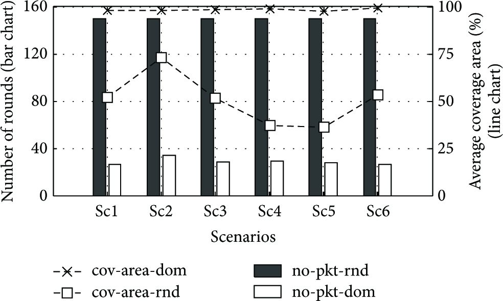
The number of rounds for ${\mathcal{A}}_{\gamma }$ (no-pkt-dom) and random approach (no-pkt-rnd) and the average coverage area estimation for ${\mathcal{A}}_{\gamma }$ (cov-area-dom) and random approach (cov-area-rnd) in different scenarios.

Increasing the marginal extension angle, ϵ, still provides a satisfactory coverage area estimation, while reducing the number of messages. We tested the performance of our proposed algorithm with different marginal extension angles in all the mentioned scenarios. As shown in Figure 16, by increasing ϵ, the number of rounds decreases, since by enlarging the angle, more search space is filtered out and consequently less packets are needed to be broadcast.

Figure 16

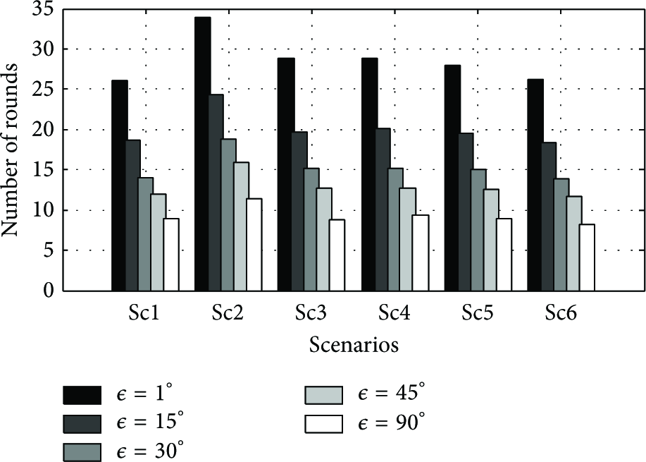
The number of rounds in ${\mathcal{A}}_{\gamma }$ with different marginal extension angle, ϵ.

However, increasing ϵ might diminish the performance of the algorithm in terms of estimated coverage area. Figure 17 shows the performance degradation by increasing the ϵ up to $\mathrm{9}{\mathrm{0}}^{\circ }$ . Under the latter setting, the proposed algorithm is able to cover around 70% of the active region. In addition to the shown value of ϵ in the graph, we also ran the simulation for $ϵ=\{{\mathrm{5}}^{\circ },\mathrm{1}{\mathrm{0}}^{\circ }\}$ and took the standard deviation of the average coverage area for $ϵ=({\mathrm{1}}^{\circ }:ϵ)$ . Since the results for $ϵ=\{{\mathrm{5}}^{\circ },\mathrm{1}{\mathrm{0}}^{\circ }\}$ were very close to the case where $ϵ={\mathrm{1}}^{\circ }$ , the coverage area computed by these values is not shown in the figure. As can be seen in Figure 17, $ϵ=\mathrm{1}{\mathrm{5}}^{\circ }$ has the smallest standard deviation (smaller than 0.65), which suggests that the coverage area computed by $ϵ=\mathrm{1}{\mathrm{5}}^{\circ }$ leads to the same coverage area as given by $ϵ={\mathrm{1}}^{\circ }$ , while at the same time using $ϵ=\mathrm{1}{\mathrm{5}}^{\circ }$ requires much smaller number of rounds compared with $ϵ={\mathrm{1}}^{\circ }$ setting, as shown in Figure 16.

Figure 17

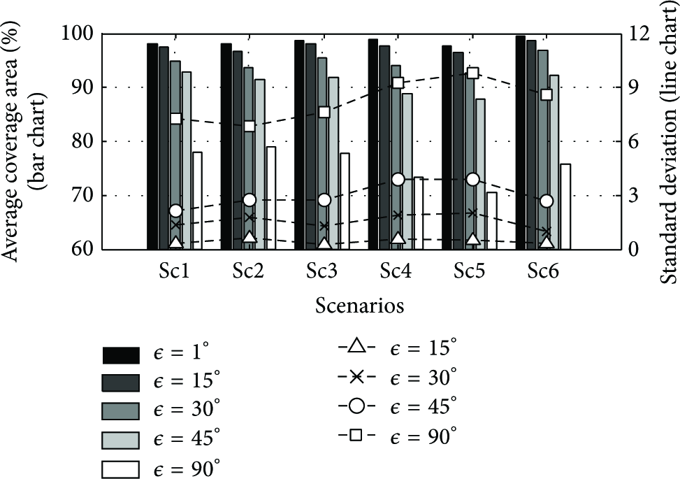
The average of estimated coverage area with different marginal extension angle, ϵ, and its standard deviation.

Figure 18 shows the execution time of vector augmenting function ${\mathcal{A}}_{\gamma }$ in an MBD network. In this experiment we set $ϵ=\mathrm{1}{\mathrm{5}}^{\circ }$ . As expected, the proposed ripple-based approach provides faster detection than the cluster-based approach for any communication range setting. Comparing Figures 14 and 18 reveals that while there are severe fluctuations in the execution time of ${\mathcal{A}}_{\beta }$ for discussed scenarios, the execution time of ${\mathcal{A}}_{\gamma }$ is almost the same in all scenarios. The reason is that, unlike ${\mathcal{A}}_{\gamma }$ , the number of required rounds in ${\mathcal{A}}_{\beta }$ depends on the number and the location of active regions. The same reasoning is also applied to Figures 12 and 16.

Figure 18

Execution time of ${\mathcal{A}}_{\gamma }$ ( $\gamma =\mathrm{1},ϵ=\mathrm{1}{\mathrm{5}}^{\circ }$ ) in an MBD network with different communication ranges for cluster-based approach: $\left\{\mathrm{C}(\mathrm{14,7}),\mathrm{C}(\mathrm{40,20})\right\}$ , and ripple-based approach: $\left\{\mathrm{R}(\mathrm{14}),\mathrm{R}(\mathrm{40})\right\}$ .

6.4. Noncircular Active Regions

As discussed in Section 4.3, ${\mathcal{A}}_{\delta }$ helps in finding the boundary of a noncircular active region, instead of identifying circular active regions from a complex shape.

Figure 19 shows the comparison of the performance of distance augmenting function with the joint augmenting function. For scenarios where a number of active regions lie very close to each other, the number of rounds required by ${\mathcal{A}}_{\beta }$ is $\mathrm{20}\%$ more than that for ${\mathcal{A}}_{\delta }$ . For more sparse events, the number of rounds required by ${\mathcal{A}}_{\beta }$ is $\mathrm{50}\%$ less compared with ${\mathcal{A}}_{\delta }$ . This happens due to the higher number of iterations that are needed to be performed by ${\mathcal{A}}_{\delta }$ to find the boundary of more than one complex shape. It should be noted that ${\mathcal{A}}_{\delta }$ is able to find the boundary of a noncircular active region and detects it as one region instead of a group of several close active regions.

Figure 19

${\mathcal{A}}_{\beta }$ versus ${\mathcal{A}}_{\delta }$ , dash lines show the boundaries provided by ${\mathcal{A}}_{\delta }$ and solid lines refer to active regions detected by ${\mathcal{A}}_{\beta }$ : (a) $\beta =\mathrm{30}$ , $\gamma =\mathrm{0.3}$ ; (b) $\beta =\mathrm{30}$ , $\gamma =\mathrm{0.2}$ , with $\beta =\mathrm{10}$ for ${\mathcal{A}}_{\beta }$ .

Comparison of vector augmenting function and joint augmentation is shown in Figure 20. It is evident that the combined approach helps in demarcating different active regions while ${\mathcal{A}}_{\gamma }$ detects the overall outer boundary. Figure 21 shows the execution time of the augmenting functions ${\mathcal{A}}_{\beta }$ , ${\mathcal{A}}_{\gamma }$ , and ${\mathcal{A}}_{\delta }$ in an MBD network for cluster-based and ripple-based approaches with different communication range for the scenarios given in Figures 20(a) and 20(b). We observe that for scenarios with overlapping events ${\mathcal{A}}_{\delta }$ converge faster, while ${\mathcal{A}}_{\beta }$ outperforms other augmenting functions for scenarios with sparse events.

Figure 20

${\mathcal{A}}_{\gamma }$ versus ${\mathcal{A}}_{\delta }$ , dash lines show the boundaries provided by ${\mathcal{A}}_{\delta }$ and solid lines refer to that given by ${\mathcal{A}}_{\gamma }$ : (a) $\beta =\mathrm{30}$ , $\gamma =\mathrm{0.3}$ ; (b) $\beta =\mathrm{30}$ , $\gamma =\mathrm{0.2}$ , with $ϵ=\mathrm{1}{\mathrm{5}}^{\circ }$ for ${\mathcal{A}}_{\gamma }$ .

Figure 21

Execution time of different augmenting functions in an MBD network with different communication ranges for cluster-based approach $\left\{\mathrm{C}(\mathrm{14,7}),\mathrm{C}(\mathrm{40,20})\right\}$ and ripple-based approach $\left\{\mathrm{R}(\mathrm{14}),\mathrm{R}(\mathrm{40})\right\}$ : (a) considering scenarios depicted in Figure 20(a) and (b) considering scenarios depicted in Figure 20(b).

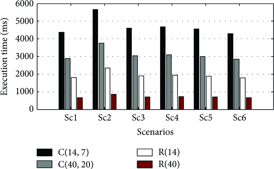
We further examined the cluster-based and ripple-based approaches to compare the time needed to extract different features according to the augmenting functions given in Section 4 for a single scenario. Figure 22 shows the elapsed time for different augmenting functions $({\mathcal{A}}_{\beta },{\mathcal{A}}_{\gamma },{\mathcal{A}}_{\delta })$ for the sample scenario sc2 over a $\mathrm{100}\times \mathrm{100}$ network. We chose this scenario because, according to the results in Section 6, this scenario includes the most complex field. It is evident that for all communication range settings and for all augmenting functions the proposed ripple-based approach outperforms the classical cluster-based approach.

Figure 22

The computation time of various feature extraction techniques ( ${\mathcal{A}}_{\beta }$ , ${\mathcal{A}}_{\gamma }$ , and ${\mathcal{A}}_{\delta }$ ) for scenario sc2 with ${\pi }_s=\mathrm{20}\%$ , $ϵ={\mathrm{15}}^{\circ }$ ,   $\gamma =\mathrm{1}$ , and   $\theta =\pi /\mathrm{4}$ .

6.5. The Impact of Network Density

Finally, we compared our techniques under various network densities. As our techniques only depend on collecting the global extrema of various augmenting functions, the results indicate that increasing the network density has almost no impact on the number of rounds. Figure 23 shows the number of rounds required in each technique with respect to the network size. The slight variation in the number of rounds is due to the effect of termination condition in ${\mathcal{A}}_{\beta }$ and the randomness in the choice of θ in ${\mathcal{A}}_{\gamma }$ .

Figure 23

The impact of density on the performance of each technique for scenario sc2.

Figure 24

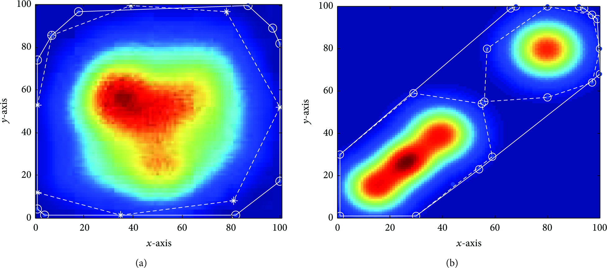
Six scenarios with different active regions; each sensor node sets the value of $\beta =\mathrm{10}$ to compute its priority—see (2)–(4). Each circle represents one filtering zone that is computed by two readings from the sensor network and excludes sensor nodes located inside the circle from participation in the future iteration(s) of the algorithm. ${\pi }_s$ is set to $\mathrm{10}\%$ of the global maximum value.

Figure 25

Six scenarios with different active regions; solid lines show the boundary computed by our algorithm with $ϵ={\mathrm{1}}^{\circ }$ and 40 iterations of the algorithm and dash lines show the boundary computed by the random algorithm with 150 random readings.

6.6. Alternative Flooding Approaches

Many emerging cyber physical systems need mechanisms to share and process data among all devices in the network. The ripple-based approach, proposed in this work, is one of such mechanisms, in the sense that it computes an aggregate quantity over all the devices. Chaos [36] and Low-Power Wireless Bus (LWB) [37] are two other examples of such mechanisms that build their data collection or dissemination capabilities based on the Glossy protocol [35].

Since we aim at obtaining an efficient and scalable algorithm with low time-complexity, we compare the performance of different flooding approaches based on execution time and scalability. Chaos outperforms LWB in terms of completion time [36]. In fact, Chaos is able to collect small amounts of data, such as a $\mathrm{1}$ -byte payload, from a $\mathrm{100}$ -node network within less than $\mathrm{100}$  ms. We believe that there are two main advantages of our proposed ripple-based approach over Chaos. Firstly, it provides a faster execution time; considering the tournament duration $\mathrm{6399}$  μs (see Section 6.1), in the ripple-based approach, all nodes will knowMIN in at most $\mathrm{52}$  ms within a seven-hop network deployment. Secondly, it offers better scalability; in fact while in Chaos the number of nodes is limited to $\mathrm{856}$ in a SBD (unless some data compression mechanism is applied), our ripple-based approach does not limit the number of involved devices.

7. Conclusions

Low-Power Wireless Sensor networks enable many emerging applications that need thousands of sensor nodes for control and monitoring. In this paper, we presented a set of techniques that identify various features in the distribution of sensed physical quantities over a dense deployment of sensor nodes. With such simple yet effective modifications, we can obtain the location and shapes of active regions with a number of messages proportional to the properties of the field. Our feature extraction techniques are efficient in the sense that they collect data from just the sensors that have more effective information for revealing the status of the monitored area.

We then proposed a fully distributed approach to make our feature extraction scale with large dense networks, where sensor nodes lie in a multiple broadcast area, and compared our method with the traditional clustering approach.

There are two main directions for our future work. The first involves investigating the temporal behavior of the extracted features, that is, developing efficient algorithms to detect and predict an evolving spatial active region. This may require detection of change dynamics and implement them within the feature extraction algorithm. The second direction leads towards the implementation of the algorithm itself. An experiment is required, using a test bed, to implement a dense sensor network to observe a phenomena and verify the results here. Along with this line, improvements to the proposed feature extraction algorithm would be required, by developing a proper synchronization algorithm for the MBD network, in order to increase its reliability. Furthermore, the limitations imposed by communication medium may also have to be considered.