Adaptive Localization in Wireless Sensor Network through Bayesian Compressive Sensing

Abstract

The estimation of the localization of targets in wireless sensor network is addressed within the Bayesian compressive sensing (BCS) framework. BCS can estimate not only target locations but also noise variance of the environment. Furthermore, we provide adaptive iteration BCS localization (AIBCSL) algorithm, which is based on BCS and will choose measurement sensors according to the environment adaptively with only an initial value, while other frameworks require prior knowledge such as target numbers to choose measurements. AIBCSL suppose that environment noise variance is identical in interested area in a short period of time and change measurement numbers until terminal condition is reached. To suppress noise, we optimize estimation result by energy threshold strategy (ETS), which takes that transmit energy of noise focused on single grid is much lower than signal into consideration. And multisnapshot BCS (MT-BCS) will be explained and lead to a good result in low SNR level situation.

1. Introduction

Wireless sensor network (WSN) has enjoyed tremendous popularity in the last decades [1, 2]. Around it there are lots of subjects. Estimating the localization of target in wireless sensor network is one of the hot topics [3]. Localization subject in most of self-organization networks has experienced excited discussion in both single target environment [4] and multitargets [5] environment, although the location of target is known to sources in some situations which are merely for data aggregation or system management, such as networks based on industrial wireless communication protocol WIA-PA [6]. Wireless network localization often appears in smart applications or tracking system such as road traffic monitoring, health monitoring, or military target tracking, which have enjoyed tremendous popularity. State-of-the-art paper gives to the interested reader several effective approaches proposed in the last decades for localization in WSN. The measurement techniques in wireless sensor network localization can be classified into three categories [3], which include angle-of-arrival estimation (AOA), distance related measurements, and RSS profiling techniques. However, the custom methods lead to poor performance in multitargets situation.

In this paper, we will introduce a novel method to wireless sensor network localization. We assume that target numbers are far less than the number of grids utilized to represent the locations of the targets. Thus target locations could be considered as sparse signal. We will consider using Bayesian compressive sensing (BCS) standpoint to solve the localization problem. BCS originated from custom compressive sensing (CS), while it employs Bayesian formalism to estimate the underlying signal. CS theory has been applied to the area of localization or target counting in [7]. However, there is no information showing that BCS method has been introduced to wireless sensor network localization. BCS have many merits compared to custom CS: (i) BCS provides not only estimation result of sparse signal but also the error message (also be known as error bars); (ii) the BCS framework provides an estimate for the posterior density function of additive noise encountered when implementing the compressive measurements. BCS algorithm is better than many other custom CS algorithms such as OMP, L1-norm, and LASSO. Another attractive advantage is that BCS is suitable for developing adaptive method by using message from error bars. Our paper analyzes the basis of BCS and introduces an adaptive iteration BCS method later. Adaptive iteration BCS will improve the accuracy of localization compared to BCS, which can be seen in the simulation section. Except for that, our paper proposes an energy threshold strategy for postprocess and yields good effect.

The original work about CS is [8]. CS is a novel sampling theory that can reconstruct s sparse signal from a small number of measurements [9]. There are many methods for recovering signal from sparse signal, which include L1-norm in [8], OMP in [10], and LASSO in [11]. Reference[7] has applied CS to the area of target count and localization in wireless sensor network, that is, the first paper to rigorously justify the validity of the problem formulation of CS localization in wireless sensor network. Since CS is put forward, there are many branches from it, such as distributed CS and Bayesian CS. Reference [12] is a work of using distributed CS in wireless sensor network localization. Bayesian compressive sensing was proposed by Ji and Xue in 2008 [13]. Bayesian compressive sensing uses Bayesian standpoint to explain CS problem and has never been seen in the area of wireless sensor network. Reference [14] comes up with an adaptive Bayesian compressed sensing algorithm and applied it to wireless network. Reference [15] executed DOA estimate by Bayesian estimate in antenna array, which directly links measurements with signal directions and an energy method could been applied. Reference [16] utilized a hierarchical form of the Laplace prior to model the sparsity of the unknown signal and in that way provided a method to estimate the localization by BCS in this paper. From another perspective, CS is welcome in the area of multitarget localization [17].

The organization of this paper is as follows. In Section 2, we will first explain the basis of BCS and multisnapshot BCS. Localization model and adaptive iteration BCS algorithm is demonstrated in the second part of Section 2. Section 3 is our simulation work and Section 4 concludes merits and application scenarios of our method.

2. Materials and Methods

2.1. Bayesian Compressive Sensing

Compressive sensing (CS) theory implies that if a signal has a sparse representation by a certain basis then it can be recovered from fewer measurements than Nyquist sampling theorem. A signal $x\in R^N$ will be represented by a $N\times N$ transform basis Ψ and a sparse signal s, formulizing that

$$\begin{array}{cc}& x=\Psi s.\end{array}$$

(1)

If s has only K entries ( ${‖s‖}_{\mathrm{0}}=K$ ) with $K\ll N$ being not equal zero, signal x is called K-sparse. Assume we get measurements $y\in R^N$ ; y and x are expressed to be linear formula:

$$\begin{array}{cc}& y=\Phi x=\Phi \Psi s=\Theta s,\end{array}$$

(2)

where Φ is $M\times \mathrm{1}$ measurement vector, such that Θ is a $M\times N$ projection matrix. Take zero mean Gaussian noise $\epsilon ~N(\mathrm{0},{\delta }_{\epsilon }^{\mathrm{2}})$ into consideration:

$$\begin{array}{cc}& y=\Theta s+\epsilon .\end{array}$$

(3)

Equation (3) depicts the projection of sparse signal s and measurements y. If we can recover y of N dimension from s of M dimension, then less memory costs and calculation costs will be taken.

2.1.1. Single-Snapshot BCS-Based Sparse Signal Estimation (ST-BCS)

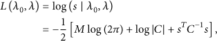
Bayesian compressive sensing (BCS) will recover y from Bayesian estimation standpoint. Because ε is a zero mean Gaussian random, the likelihood model of recovering y from s is

$$\begin{array}{cc}& p(y\hspace{0.17em}|\hspace{0.17em}s,{\delta }_{\epsilon }^{\mathrm{2}})={\left(\mathrm{2}\pi {\delta }_{\epsilon }^{\mathrm{2}}\right)}^{-M/\mathrm{2}}\exp \left(-\frac{\mathrm{1}}{\mathrm{2}{\delta }_{\epsilon }^{\mathrm{2}}}{‖y-\Theta s‖}^{\mathrm{2}}\right).\end{array}$$

(4)

According to Bayesian estimation theorem, the analysis of CS problem turns out to be a priori constrained optimization problem. The priori condition is that s is a sparse vector ( ${‖s‖}_{\mathrm{0}}=K$ ). The posterior probability [16] is

$$\begin{array}{cc}& p\left(s\hspace{0.17em}|\hspace{0.17em}\lambda \right)={\displaystyle \prod }_{i=\mathrm{1}}^{N}N\left(s_i\hspace{0.17em}|\hspace{0.17em}\mathrm{0},{\lambda }_i^{-\mathrm{1}}\right),\end{array}$$

(5)

where $N(s_i\hspace{0.17em}|\hspace{0.17em}\mathrm{0},{\lambda }_i^{-\mathrm{1}})$ means that $s_i$ is Gaussian random where mean is zero and variance is ${\lambda }_i^{-\mathrm{1}}$ . $\lambda =\left[{\lambda }_{\mathrm{1}},{\lambda }_{\mathrm{2}},\dots ,{\lambda }_N\right]$ is super-parameters at the service of solving priori probability, which will control the sparse level of s.

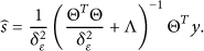
BCS provides a method to estimate s and even noise covariance by only a few measurements y through maximize posterior probability. In that viewpoint, posterior probability of s and ${\delta }_{\epsilon }^{\mathrm{2}}$ are maximized; that is, $\widehat{s}=\arg \left\{{\max }_{s}p\left([s,{\delta }_{\epsilon }^{\mathrm{2}},\lambda ]\hspace{0.17em}|\hspace{0.17em}y\right)\right\}$ . Posterior probability is

$$\begin{array}{cc}& p\left([s,{\delta }_{\epsilon }^{\mathrm{2}},\lambda ]\hspace{0.17em}|\hspace{0.17em}y\right)=p(s\hspace{0.17em}|\hspace{0.17em}{\delta }_{\epsilon }^{\mathrm{2}},y,\lambda )p\left([{\delta }_{\epsilon }^{\mathrm{2}},\lambda ]\hspace{0.17em}|\hspace{0.17em}y\right).\end{array}$$

(6)

$p(s\hspace{0.17em}|\hspace{0.17em}{\delta }_{\epsilon }^{\mathrm{2}},y,\lambda )$ provides the estimation of s, and $p([{\delta }_{\epsilon }^{\mathrm{2}},\lambda ]\hspace{0.17em}|\hspace{0.17em}y)$ gives the result of noise estimation. Our target is maximizing the first item [16]. Formulize it by multivariable Gaussian distribution [16]:

$$\begin{array}{l}p(s\hspace{0.17em}|\hspace{0.17em}{\delta }_{\epsilon }^{\mathrm{2}},y,\lambda )\\ \hspace{1em}={\left(\mathrm{2}\pi \right)}^{-\left(M+\mathrm{1}\right)/\mathrm{2}}{\left|\Sigma \right|}^{-\mathrm{1}/\mathrm{2}}\exp \left(-\frac{\mathrm{1}}{\mathrm{2}}{\left(\widehat{s}-\mu \right)}^T{\left|\Sigma \right|}^{-\mathrm{1}}\left(\widehat{s}-\mu \right)\right),\end{array}$$

(7)

where mean and covariance are

$$\begin{array}{cc}& \mu =\frac{\mathrm{1}}{{\delta }_{\epsilon }^{\mathrm{2}}}\Sigma {\Theta }^{T}y,\\ \Sigma ={\left[\frac{\mathrm{1}}{{\delta }_{\epsilon }^{\mathrm{2}}}{\Theta }^T\Theta +\Lambda \right]}^{-\mathrm{1}},\hspace{1em}\hspace{1em}\Lambda =\mathrm{diag}({\lambda }_{\mathrm{1}},{\lambda }_{\mathrm{2}},\dots ,{\lambda }_N).\end{array}$$

(8)

Thus, we must first estimate u and Σ to accomplish the task above. Assuming ${\lambda }_{\mathrm{0}}=\mathrm{1}/{\delta }_{\epsilon }^{\mathrm{2}}$ , we use maximum likelihood estimation (MLE) to get parameters ${\lambda }_{\mathrm{0}},\lambda$ . The logarithm function is

$$\begin{array}{ll}L\left({\lambda }_{\mathrm{0}},\lambda \right)& =\log \left(s\hspace{0.17em}|\hspace{0.17em}{\lambda }_{\mathrm{0}},\lambda \right)\\ & =-\frac{\mathrm{1}}{\mathrm{2}}\left[M\log \left(\mathrm{2}\pi \right)+\log \left|C\right|+s^T{C}^{-\mathrm{1}}s\right],\end{array}$$

(9)

where $C={\delta }^{\mathrm{2}}I+\Theta {\Lambda }^{-\mathrm{1}}{\Theta }^T$ and I is eye matrix. $\max L({\lambda }_{\mathrm{0}},\lambda )$ with respect to ${\lambda }_{\mathrm{0}}$ and λ will get iteration relationship as below:

$$\begin{array}{cc}& {\lambda }_i^{\text{new}}=\frac{\mathrm{1}-{\lambda }_i{\Sigma }_{ii}}{{\mu }_i^{\mathrm{2}}},\hspace{1em}i\in \{\mathrm{1,2},\dots ,N\},\\ {\lambda }_{\mathrm{0}}^{\text{new}}=\frac{M-{\sum }_{i=\mathrm{1}}^N(\mathrm{1}-{\lambda }_i{\Sigma }_{ii})}{{‖y-\Theta \mu ‖}_{\mathrm{2}}^{\mathrm{2}}},\end{array}$$

(10)

where ${\Sigma }_{ii}$ is ith diagonal element of Σ. Given the initial values of ${\lambda }_{\mathrm{0}},\lambda$ , update Σ and μ by (8) and (10) until convergence. For the reason that BCS will return with Σ, it is superior to custom CS method when applied to adaptive estimate. BCS estimation result is [15]

$$\begin{array}{cc}& \widehat{s}=\frac{\mathrm{1}}{{\delta }_{\epsilon }^{\mathrm{2}}}{\left(\frac{{\Theta }^T\Theta }{{\delta }_{\epsilon }^{\mathrm{2}}}+\Lambda \right)}^{-\mathrm{1}}{\Theta }^{T}y.\end{array}$$

(11)

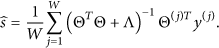
2.1.2. Multisnapshot BCS-Based Sparse Signal Estimation (MT-BCS)

To suppress the noise, take the relevant of more than one signal in a short period of time into account. Do W samples at W different times, and then

$$\begin{array}{cc}& y_t=\Theta s_t+{\epsilon }_t,\hspace{1em}t=\{\mathrm{1,2},\dots ,W\}.\end{array}$$

(12)

Maximizing posterior of s turns to be

$$\begin{array}{cc}& \widehat{s}=\frac{\mathrm{1}}{W}{\displaystyle \sum }_{t=\mathrm{1}}^W\arg \left\{\underset{s_t}{\max }p\left([s_t,{\delta }_{\epsilon }^{\mathrm{2}},\lambda ]\hspace{0.17em}|\hspace{0.17em}{y}_t\right)\right\},\hspace{1em}t=\{\mathrm{1,2},\dots ,W\}.\end{array}$$

(13)

Super-parameters can iterated by following equations:

$$\begin{array}{cc}& {\lambda }_i^{\text{new}}=\frac{W-{\lambda }_i{\sum }_{j=\mathrm{1}}^W{\Sigma }_{ii}^{\left(j\right)}}{{\sum }_{j=\mathrm{1}}^W{\mu }_i^{\mathrm{2}\left(j\right)}},\hspace{1em}i\in \{\mathrm{1,2},\dots ,N\},\\ {\lambda }_{\mathrm{0}}^{\text{new}}=\frac{{\sum }_{j=\mathrm{1}}^W\left\{M-{\sum }_{i=\mathrm{1}}^N(\mathrm{1}-{\lambda }_i{\Sigma }_{ii}^{\left(j\right)})\right\}}{{\sum }_{j=\mathrm{1}}^W{‖y^{\left(j\right)}-{\Theta }^{\left(j\right)}{\mu }^{\left(j\right)}‖}_{\mathrm{2}}^{\mathrm{2}}}.\end{array}$$

(14)

Similarly but not the same, estimated result of s is as below in MT-BCS:

$$\begin{array}{cc}& \widehat{s}=\frac{\mathrm{1}}{W}{\displaystyle \sum }_{j=\mathrm{1}}^W{\left({\Theta }^T\Theta +\Lambda \right)}^{-\mathrm{1}}{\Theta }^{\left(j\right)T}{y}^{\left(j\right)}.\end{array}$$

(15)

2.2. Location Sensing Formulation

2.2.1. Localization Model

First we divide localization area to be $N=nx\times ny$ grids. Then assign index for grids from 1~N as Figure 1. The coordinate of index is calculated by

$$\begin{array}{cc}& x\left(i\right)=\mathrm{mod}\left(i,nx\right),\\ y\left(i\right)=i-\mathrm{mod}(i,nx)+\mathrm{1}.\end{array}$$

(16)

Assume T targets (also known as sources) are distributed sporadic in those areas, such that they can be represented by a sparse vector $s={\left[s_{\mathrm{1}},s_{\mathrm{2}},\dots ,s_N\right]}^T$ , where $s_i$ represents the energy of target in ith grid area. If there is no target in ith grid, $s_i=\mathrm{0}$ .

Figure 1

Localization girds and index.

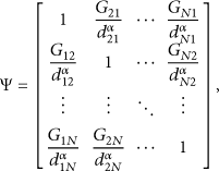
Energy attenuation [3] from ith grid to jth gird is

$$\begin{array}{cc}& P_r\left(d_{ij}\right)=\left\{\begin{array}{cc}{P}_i\frac{G_{ij}}{d_{ij}^{\alpha }},\hfill & d_{ij}>d_{\mathrm{0}}\hfill \\ P_i,\hfill & d_{ij}\le d_{\mathrm{0}},\hfill \end{array}\right.\end{array}$$

(17)

where $P_i$ is signal intensity in ith grid and $d_{\mathrm{0}}$ is a very short reference distance. $d_{ij}$ is Euclidean distance from ith grid to jth gird. $G_{ij}$ is Rayleigh fading factor from i to j which is related to specific environment. α is distance factor, often choose between [2.0, 5.0].

Combining (1) and (13),

$$\begin{array}{cc}& \Psi =\left[\begin{array}{cccc}\mathrm{1}& \frac{G_{\mathrm{21}}}{d_{\mathrm{21}}^{\alpha }}& \cdots & \frac{G_{N\mathrm{1}}}{d_{N\mathrm{1}}^{\alpha }}\\ \frac{G_{\mathrm{12}}}{d_{\mathrm{12}}^{\alpha }}& \mathrm{1}& \cdots & \frac{G_{N\mathrm{2}}}{d_{N\mathrm{2}}^{\alpha }}\\ ⋮& ⋮& \ddots & ⋮\\ \frac{G_{\mathrm{1}N}}{d_{\mathrm{1}N}^{\alpha }}& \frac{G_{\mathrm{2}N}}{d_{\mathrm{2}N}^{\alpha }}& \cdots & \mathrm{1}\end{array}\right],\end{array}$$

(18)

$$\begin{array}{cc}& s={\left[P_{\mathrm{1}},P_2,\dots ,P_N\right]}^T.\end{array}$$

(19)

The signal $x={\left[x_{\mathrm{1}},x_{\mathrm{2}},x_{\mathrm{3}},\dots ,x_N\right]}^T$ is the energy intensity in ith gird. According CS theorem, M ( $k<M\ll N$ ) measurements that satisfy RIP rules [8] are able to recover signal without loss. Thus, we deploy M sensors in interested areas. In (2), if there is sensor in grid j, $\Phi (i,j)=\mathrm{1}$ ; otherwise, $\Phi (i,j)=\mathrm{0}$ . We also need consider noise such as (3).

2.2.2. BCS Based Adaptive Localization

Compared with custom CS method, BCS not only provides sparse estimation result, but also gives estimation of noise. In this section, we develop an adaptive BCS algorithm that will choose measurements adaptively for target localization in wireless sensor network. The algorithm assumes that noises in the interested area are consistent, which means that the variances of noise in anywhere of interested area are identical in a short period of time. Measurement numbers change based on the feedback of variances of noise by BCS estimation, until the inconsistency of variances comes to be a small value.

At the beginning, we choose $M_{\mathrm{1}}$ sensors randomly (that is an initial value) by primary device to acquire signal from interested gird area. The BCS estimated noise variance of those sensors is ${\delta }^{(\mathrm{1})\mathrm{2}}=\{{\delta }_{\mathrm{1}}^{\left(\mathrm{1}\right)\mathrm{2}},{\delta }_{\mathrm{2}}^{\left(\mathrm{1}\right)\mathrm{2}},\dots ,{\delta }_{K^{\left(\mathrm{1}\right)}}^{\left(\mathrm{1}\right)\mathrm{2}}\}$ , where $K^{(\mathrm{1})}$ means that signal is $K^{(\mathrm{1})}$ -sparse at the first iteration. We develop a constraint condition then, and $dM$ sensors will be increased from the next iteration if that condition is not satisfied. The approach of choosing the $dM$ sensors comes to two situations: (i) if there is no sensor in the grid area localized by BCS at the last iteration, we will increase a measurement in that grid and (ii) if there have been sensor in the grid area localized by BCS at the last iteration, we choose another grid that without been measured randomly. Set Bayesian estimation error ${\delta }^{(a)2}=\{{\delta }_1^{(a)2},{\delta }_2^{(a)2},\dots ,{\delta }_{K^{(a)}}^{(a)2}\}$ at the ath iteration, where $K^{(a)}$ means that signal is $K^{(a)}$ -sparse. There are two iteration termination (constraint) conditions used in our paper. One of them is the comparison of ${\xi }_{\mathrm{1}}$ with threshold ${\eta }_{\mathrm{1}}$ , and the expression of ${\xi }_{\mathrm{1}}$ is

$$\begin{array}{cc}& {\xi }_{\mathrm{1}}=\left\{\begin{array}{cc}‖\frac{{\delta }_{{\delta }^{\left(a\right)2}}}{{\mu }^{\left(a\right)}}-\frac{{\delta }_{{\delta }^{(a-1)\mathrm{2}}}}{{\mu }^{(a-1)}}‖,\hfill & {\mu }^{\left(a\right)},{\mu }^{(a-\mathrm{1})}\ne \mathrm{0}\hfill \\ \mathrm{0},\hfill & {\mu }^{\left(a\right)}\hspace{0.17em}\hspace{0.17em}\text{or}\hspace{0.17em}\hspace{0.17em}{\mu }^{(a-\mathrm{1})}=\mathrm{0}.\hfill \end{array}\right.\end{array}$$

(20)

${\xi }_{\mathrm{1}}$ represents the convergence rate in some degree, which put forward that the mean and variance change little at the convergence process. Second, consider that the Gaussian random is identical anywhere in the interested area, such that we let ${\xi }_{\mathrm{2}}={\delta }_{{\delta }^{(a)\mathrm{2}}}$ be reasonable. The combination of ${\xi }_{\mathrm{1}}$ and ${\xi }_{\mathrm{2}}$ comes to be

$$\begin{array}{cc}& \xi =\left\{\begin{array}{cc}{\xi }_{\mathrm{1}}<{\eta }_{\mathrm{1}},\hspace{0.17em}\hspace{0.17em}{\xi }_{\mathrm{2}}<{\eta }_{\mathrm{2}},\hfill & \text{Strongest}\hspace{0.17em}\hspace{0.17em}\text{condition}\hfill \\ {\xi }_{\mathrm{1}}<{\eta }_{\mathrm{1}}\hfill & \hfill \\ {\xi }_{\mathrm{2}}<{\eta }_{\mathrm{2}}\hfill & \hfill \\ {\xi }_{\mathrm{1}}<{\eta }_{\mathrm{1}}\hspace{0.17em}\hspace{0.17em}\text{or}\hspace{0.17em}\hspace{0.17em}{\xi }_{\mathrm{2}}<{\eta }_{\mathrm{2}},\hfill & \text{Weakest}\hspace{0.17em}\hspace{0.17em}\text{condition}.\hfill \end{array}\right.\end{array}$$

(21)

Algorithm 1 gives the whole adaptive algorithm procedure.

Algorithm 1: Adaptive iteration BCS localization (AIBCSL).

$$(\mathit{1}$$ )  Set   $${\xi }_{\mathrm{1}}=Inf$$ , $${\xi }_{\mathrm{2}}=Inf$$ , $$a=\mathrm{1}$$ , Given initial sensor number $$M=M_{\mathrm{1}}$$

( $$\mathit{2}$$ )   $$R=randperm(N)$$ . Set $$\{M_{\mathrm{1}}\}=R\left[\mathrm{1}:M_{\mathrm{1}}\right]$$ .

( $$\mathit{3}$$ )  While   $$a<\max \_iteration$$ and ξ is false

( $$\mathit{4}$$ )    Update Θ.

( $$\mathit{5}$$ )     $$\left\{s,idx,K^{(a)},{\delta }^{(\mathrm{a})\mathrm{2}}\right\}=\text{BCS}\left({\mathrm{M}}_a,\mathrm{\Theta }\right)$$ .

( $$\mathit{6}$$ )    Determine mean and variance of $${\delta }^{(\mathrm{a})\mathrm{2}}=\left\{{\delta }_{\mathrm{1}}^{(\mathrm{a})\mathrm{2}},{\delta }_{\mathrm{2}}^{(\mathrm{a})\mathrm{2}},\dots ,{\delta }_{Ka}^{(\mathrm{a})\mathrm{2}}\right\}$$

     $${\mu }^{(\mathrm{a})}=\frac{\mathrm{1}}{K^{(a)}}{\displaystyle \sum }_{i=\mathrm{1}}^{K^{(a)}}{\delta }_i^{(a)\mathrm{2}},{\delta }_{{\delta }^{(a)\mathrm{2}}}=\frac{\mathrm{1}}{K^{(a)}}{\displaystyle \sum }_{i=\mathrm{1}}^{K^{(a)}}{\left({\delta }_i^{(a)\mathrm{2}}-{\mu }^{(\mathrm{a})}\right)}^{\mathit{2}}$$

( $$\mathit{7}$$ )    Calculate ξ by (21).

( $$\mathit{8}$$ )     $$a=a+\mathrm{1}$$

(9)     $$dM=length(idx)$$ , $$M_{a+\mathrm{1}}=M_a+dM$$

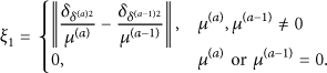
(10)  Increase acquisition from the added $$dM$$ sensors.

     $$\{M_{a+\mathrm{1}}\}=unique\{M_a,idx,R\left[~\right]\}$$ , where $$R\left[~\right]$$ contains values from R to satisfy that $$M_{a+\mathrm{1}}=M_a+dM$$ .

(11) End

(12) Return grids (locations) of target $$idx$$ .

2.2.3. Strategy to Determine Targets

According to (19), s is K-sparse vector. BCS localization returns the energy result of all N locations. Random noise will increase error rate. In this section, we assume that energy of noise source is much less than true target, such that we can estimate targets’ location by energy threshold strategy (ETS) further [15]. More specifically, the entries of estimated sparse signal are sorted according to their energy, ${\left|s_k\right|}^{\mathrm{2}},\hspace{0.17em}\hspace{0.17em}k=\mathrm{1},\dots ,K$ , from high to low, such that $id{x}_{\mathrm{1}}={\max }_k\left\{{\left|s_k\right|}^{\mathrm{2}}\right\}$ and $id{x}_K={\min }_k\left\{{\left|s_k\right|}^{\mathrm{2}}\right\}$ , where $id{x}_k$ means sort index. Setting threshold ${\eta }_s$ , algorithm only reserves parts of all targets with the maximal energy. The determined algorithm by energy threshold is depicted as Algorithm 2.

Algorithm 2: Energy threshold strategy (ETS).

$$(\mathit{1}$$ ) Set   $$k=\mathrm{1}$$ , $$S{S}_k=\mathrm{0}$$

( $$\mathit{2}$$ ) $$[S,idx]=sort({\left|{\mathrm{s}}_k\right|}^{\mathrm{2}}$$ , “descend”)

( $$\mathit{3}$$ ) While   $$k<=K$$ and $$S{S}_k<{\eta }_s$$

( $$\mathit{4}$$ )    $$S{S}_k=S{S}_k+S_k$$ ,

( $$\mathit{5}$$ )    $$k=k+\mathrm{1}$$

( $$\mathit{6}$$ ) End

( $$\mathit{7}$$ ) Return targets’ position $$\{id{x}_{\mathrm{1}},\dots ,id{x}_k\}$$

3. Results and Discussion

For the purpose of verifying aforementioned algorithms, simulations are executed in this section. Scale of interested area is 30 m × 30 m, in which we have grid size partitioned to be 1.0 m × 1.0 m. Such that there are $N=900$ grids in total. Deploy T targets in that area randomly. Assume the estimation target numbers are $\stackrel{⌢}{T}$ by BCS and coordinate is $\{\left({\stackrel{⌢}{x}}_i,{\stackrel{⌢}{y}}_i\right)\hspace{0.17em}|\hspace{0.17em}i=\mathrm{1,2},\dots ,\stackrel{⌢}{T}\}$ . We will use mean localization error (MLE) to determine the performance of localization. MLE is formulated as

$$\begin{array}{cc}& \text{MLE}=\frac{{\sum }_{i=\mathrm{1}}^{\min \{T,\stackrel{⌢}{T}\}}{‖{\left(x_i-{\stackrel{⌢}{x}}_i\right)}^{\mathrm{2}}+{\left(y_i-{\stackrel{⌢}{y}}_i\right)}^{\mathrm{2}}‖}^{\mathrm{1}/\mathrm{2}}}{\min \{T,\stackrel{⌢}{T}\}}.\end{array}$$

(22)

Because $\stackrel{⌢}{T}$ is not identical to T sometimes, we also take target number error (TNE) as a performance criterion, where TNE is

$$\begin{array}{cc}& \text{TNE}=\frac{‖T-\stackrel{⌢}{T}‖}{T}.\end{array}$$

(23)

Simulations are executed under noise situation, such that signal to noise ratio is defined:

$$\begin{array}{cc}& \text{SNR}=\mathrm{10}\log \left[\frac{{\sum }_{m=\mathrm{1}}^M{y}^{\left(\text{Noiseless}\right)}}{M{\delta }_{\epsilon }^{\mathrm{2}}}\right].\end{array}$$

(24)

3.1. BCS Simulation

Compared to custom methods, such as L1-norm [18], OMP [19], and LASSO [19], BCS is superior to them at certain circumstance. We will use CVX toolbox to implement L1-norm and SPAMs to implement OMP and LASSO in our experiments. In our simulation, each measurement is corrupted by Gaussian random according to (24). Energy threshold strategy is applied with ${\eta }_s=\mathrm{0.99}$ in this section unless otherwise specified. All custom methods give the simulation target numbers that are identical to the real target numbers at the initialization time in all of our simulation tasks. Figure 2 shows the result of single target experiment under different SNR level. The result of BCS method is better than OMP and approximate performance compared with L1-norm and LASSO.

Figure 2

MLEs in single target ( $T=1$ ) simulation. $M=20$ . Results are statistical data from 100 tests.

Figure 3 shows the MLE result of multitargets localization by BCS and custom CS methods in different SNR level. Target number $T=5$ in reality here. Setting of target number of all custom methods is 5, such that TNE is 0 of all methods except for BCS. Figure 3 proves that Bayesian is better than all of custom methods in some degree in multitarget situation.

Figure 3

MLEs in multitargets ( $T=5$ ) simulation. $M=100$ . Results are statistical data from 100 tests.

Figure 4 shows the TNE result in different SNR level for BCS method both in single target and multitargets. In single target ( $T=1$ ) situation, TNE is monotone decreasing along with SNR's increase. In multitargets situation, most of TNEs are less than 0.6 and there is little variation. We have set $\stackrel{⌢}{T}=T$ for all custom CS methods, and the TNE of them are zeros.

Figure 4

TNEs vary with SNR using BCS method. Results are statistical data from 100 tests.

Figure 5 examines the MLE under different measurements. It demonstrates directly that BCS is better than other methods for that BCS has less MLE than others. Another clue of that figure tells us that MLE is decreasing along with the increasing of measurements. Figure 6 gives the TNE result of BCS method when measurements increase. The trend of TNE is decreasing along with the increasing of measurements, such that we can improve the localization accuracy through increasing measurements until satisfying our demand.

Figure 5

MLEs under different measurements. Results are statistical data from 100 tests.

Figure 6

TNEs under different measurements using BCS method. Results are statistical data from 100 tests.

The comparison between energy threshold strategy version and the not optimized version is depicted in Figure 7. After ETS optimizing, TNEs and MLEs are smaller than the not optimized version with MLE and TNE decline of about 50%. It proves that ETS is effective in improving accuracy of localization.

Figure 7

Comparison of MLEs and TNEs between ETS version and the not optimized version. M is initial value of measurements here. Results are statistical data from 100 tests.

3.2. AIBCSL Simulation

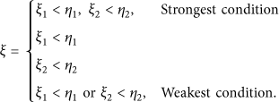
Adaptive iteration BCS localization algorithm could choose the number of sensors adaptively without user participating except for an initial value. The terminal condition used here for iteration is $\xi ={\xi }_{\mathrm{1}}<{\eta }_{\mathrm{1}}$ and ${\xi }_{\mathrm{2}}<{\eta }_{\mathrm{2}}$ , where ${\eta }_{\mathrm{1}}=\mathrm{5}*\mathrm{1}{\mathrm{0}}^{-\mathrm{3}}$ and ${\eta }_{\mathrm{2}}=\mathrm{5}*\mathrm{1}{\mathrm{0}}^{-\mathrm{3}}$ . The maximum iteration of AIBCSL is 50 in all of our simulations in this section and tests are under 100 repetition. Energy threshold strategy is applied with ${\eta }_s=\mathrm{0.99}$ .

Figure 8 shows that AIBCSL leads to less MLE and TNE. AIBCSL is superior to BCS. It almost yields perfect result (results close to zero) when SNR is greater than 20 dB. Figure 9 demonstrates visualizing that number of measurements changes adaptively according to environment with initial value $M=20$ for $T=1$ and $M=100$ for $T=5$ . With the increasing of SNR, the measurements decrease slowly, while measurements change a lot comparing $T=5$ with $T=1$ .

Figure 8

Compare AIBCSL with BCS. The initial value of measurement is 20 for $T=1$ and 100 for $T=5$ . Results are statistical data from 100 tests.

Figure 9

AIBCSL will lead to different measurements with the change of SNR. Results are statistical data from 100 tests.

Figure 10 is the iteration process of AIBCSL with different target numbers. ${\xi }_{\mathrm{1}}$ and ${\xi }_{\mathrm{2}}$ change along with iteration's increase. At the convergence time, both ${\xi }_{\mathrm{1}}$ and ${\xi }_{\mathrm{2}}$ are approximately comes to be zero. Then it terminates the iteration and returns the localization result.

Figure 10

The convergence process of ${\xi }_{\mathrm{1}}$ and ${\xi }_{\mathrm{2}}$ . Target number $T=\{\mathrm{1,3},\mathrm{5,7},\mathrm{9,11,13,15,17,19}\}$ , SNR = 25 dB. Results are statistical data from 100 tests.

With the changing of target numbers, AIBCSL choose measurements adaptively. Figure 11 shows the relationship between target numbers and measuments. Measurements at convergence are linear with target number, which means that AIBCSL could determine the measurements just according to the environment without needing any message about target numbers in advance. Figure 12 gives a snapshot of simulation process. In that figure, MLE of AIBCSL is better than OMP, L1-norm, and LASSO.

Figure 11

Converged measurements with the increasing of target number. Results are statistical data from 100 tests.

Figure 12

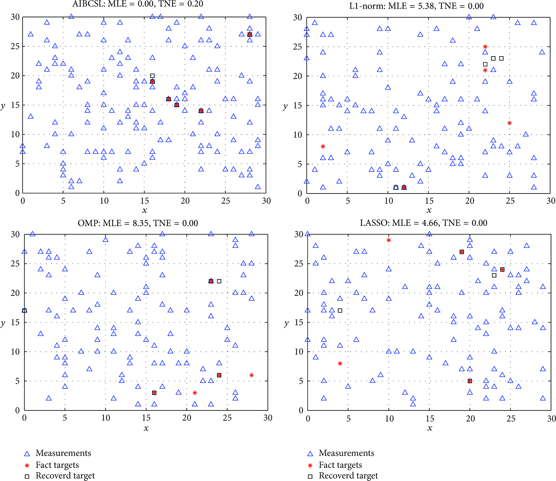
Snapshot of simulation. AIBCSL is compared with custom CS algorithms. Parameters: ${\eta }_{\mathrm{1}}=\mathrm{5}*\mathrm{1}{\mathrm{0}}^{-\mathrm{3}}$ ,   ${\eta }_{\mathrm{2}}=\mathrm{5}*\mathrm{1}{\mathrm{0}}^{-\mathrm{3}}$ , and maximum iteration is 50 for BCS. Initial target number of L1-norm, OMP, and LASSO are $T=5$ . SNR = 25 dB.

3.3. Multisnapshot Simulation

In this simulation work we will combine multisnapshot with adaptive localization algorithm proposed in Section 2, which is called MT-AIBCSL for short in this paper. In this simulation, the terminal condition is $\xi ={\xi }_{\mathrm{1}}<{\eta }_{\mathrm{1}}$ and ${\xi }_{\mathrm{2}}<{\eta }_{\mathrm{2}}$ , where ${\eta }_{\mathrm{1}}=\mathrm{5}*\mathrm{1}{\mathrm{0}}^{-\mathrm{3}}$ and ${\eta }_{\mathrm{2}}=\mathrm{5}*\mathrm{1}{\mathrm{0}}^{-\mathrm{3}}$ . Number of snapshots $W=2$ . Initial value of measurements is 20 for $T=1$ and 100 for $T=5$ . All the simulation results are based on 100 times statistics. Tests are executed on different SNR and Figure 13 shows that MT-AIBCSL reduces the MLE and TNE relative to AIBCSL, especially low SNR region. That means MT-AIBCSL is really useful for reducing noise interference.

Figure 13

Compare MT-AIBCSL with AIBCSL with different SNR.

Because MT-AIBCSL takes full advantage of correlation of time domain, it suits the situation that the environment is not varied in a short period of time. An excellent choice is applying AIBCSL to real-time requirements and low correlation of time domain situations and vice versa.

4. Conclusions

In this paper, BCS is introduced to wireless sensor network localization and the results compared with custom CS are assessed. We then proposed AIBCSL and MT-AIBCSL to improve the accuracy of localization on the basis of BCS. AIBCSL take the assumption that noise variances are identical in the interested localization area in a short period of time. And simulation results proved that method is effective in noise environment. Advantages and limitations of AIBCSL and MT-AIBCSL have been analyzed in comparison with custom CS methods. The proposed adaptive methods have demonstrated the following superiorities.

• (i)

Estimating target locations with noise variance being known at the same time.

(ii)

AIBCSL provides higher MLE and TNE than BCS and custom methods. And MT-AIBCSL is better than AIBCSL in low SNR level.

(iii)

There is no need for user to know the number of targets ahead of time and only an initial value of measurement is required by using AIBCSL and MT-AIBCSL.

Expect for that, an ETS provides performance improvement with almost 50% error decline, which is well suited for BCS framework and multitarget localization situation.