A New Two-Level Clustering Scheme for Partitioning in Distributed Wireless Sensor Networks

Abstract

Partitioning has always been a challenge in the design of distributed applications. It allows optimizing the intercommunication between the system components and so increasing the lifetime of the network. Graph theory methods have often been used to perform partitioning in classic distributed systems but seem to be not efficient in ad hoc or wireless sensor networks (WSN). The main reason is related to the topology of these kinds of networks and the presence of multihop communication. In this paper, we propose a new self-organisation of the WSN based on the optimization of the number of jumps between any sensor and the sink. The network is based on a two-level hierarchy structure and organised as a set of clusters with one cluster-head by cluster and a super-leader for the entire network. The optimisation process has been performed and validated by introducing some parameters, baptized cohesion parameters. The simulation of our approach compared to existing and previously developed protocols shows the efficiency of the method. The results are very interesting and allow projecting several perspectives to improve performances by using other metrics.

1. Introduction

WSN have widely been investigated these last years. A big number of research works such as [1–3] aim to find solutions for network structuring and managing so that to increase the lifetime of the network by minimizing the energy consumption for each node. In our work, we focus on the partitioning of distributed systems and try to study the particular case of WSN.

When designing distributed applications, we must answer the following fundamental question: how to organize and share processing, in order to optimize the execution time, as well as the use of resources. This depends on the kinds of the components (processors or process), on the communication support (wired or wireless), on the nature of exchanged data (multimedia or not), and on the constraints imposed by the application needs. WSN are considered as specific distributed systems that are composed of distributed sensors. Each sensor has to collect specific environmental information and to send them to the sink. In most cases the transmission of the data needs several hops from the sensor to the sink. So partitioning in this case consists of optimizing the routing by minimizing the number of hops. As the routing is strongly influenced by the network organisation, we have proposed the development of an approach structuring the network into clusters that aims to optimize the routing. This paper is organized as follows. Section 2 gives an outline of the partitioning concept in distributed systems in general and the principle of the use of graph theory methods to perform it and then explains the insufficiency of these methods when applied to WSN which constitutes the motivation of our approach. At the end of this section, we present the clustering solution and some related works in the field. Section 3 describes the new clustering algorithm, WSN-2-LTS; this description includes some assumptions, the metric used for the cluster-head selection, the clusters formation principle, data structures, exchanged messages followed by the commented WSN-2-LTS pseudocode, and the principle of the communication and the routing. In Section 4 we define new parameters, baptized cohesion parameters, according to our structure and communication procedures, and then show the importance of these parameters to measure the performance of the WSN and how to use them to perform the reorganization of the network. Section 5 shows the connection between the defined cohesion parameters and the partitioning. Section 6 contains the experimental results of our algorithm compared to two existing and previously developed protocols. The simulation is performed by using the network simulator NS2 (version 2.31). Section 7 concludes the paper and suggests new directions for future research.

2. Preliminaries

2.1. Partitioning in Distributed Applications

Partitioning means that we have to define the best strategy to distribute calculations on different units. These units must then share the results or/and communicate/synchronise between them. As the distributed system is composed of different units, the overall execution time of the application is influenced by the number and duration of communications between these different units. The less the communications are held, the more the execution time is decreased. Therefore, even if the partitioning is closely linked to the application needs, the objective in designing this partitioning is always to minimize the number of communications. On the other hand, as we have raised, the issue of process partitioning may have a mathematical basis or can be put back to a mathematical problem in graph theory: graph partitioning. Indeed a distributed system can be seen as a graph composed of several nodes. These nodes represent the process units, and arcs between nodes are links or communications between these units.

2.2. Graph Partitioning

The graph partitioning (GP) consists in dividing all summits of a graph into several subsets, so that these subsets are of about the same size, that's they have approximately the same number of peaks; with few connections between them. This problem is widely studied for over thirty years and has many applications, namely, design of VLSI integrated circuit, parallel computing [4], finite elements optimization method [5], and so forth. We present below the formal definition of graph partitioning.

2.2.1. Graph Partitioning Definition

Let $G=(U,Q)$ be a graph where U is the set of summits $u_i$ and Q is the set of edges $(u_i,u_j)$ . In some cases, the peaks of the graph may be associated with spatial coordinates determining their relative positions in the d-dimensional space $R^d$ . A k-partitioning of this graph is an application $F:U\to [\mathrm{1},k]$ of the peaks to the subsets (called partitions) $U_{\mathrm{1}}$ , $U_{\mathrm{2}}$ , and $U_k$ ( $F(u_i)=j$ if and only if the summit $u_i$ is in the partition $U_j$ ), where ${\bigcup }_i‍u_i=U$ and $U_i\bigcap U_j=\varphi$ , ( $i\ne j$ ).

Each partitioning result is a set of cut edges $E_c$ . The $E_c$ is defined as all edges with both ends in separate partitions, $E_c=(u_i,u_j)\hspace{0.17em}|\hspace{0.17em}(u_i\hspace{0.17em}|\hspace{0.17em}{u}_j)\in Q$ , $P(u_i)\ne P(u_j)$ . The cardinality of $E_c$ (all elements of $E_c$ ) noted $\left|E_c\right|$ is called the partitioning cutsize. The cardinality $\left|U_i\right|$ is called the size of the partition $U_i$ . We illustrate in Figure 1 an example of a 3-partitioning of a graph with a cutsize equal to 7. The problem of k-partitioning of the graph $G=(U,Q)$ is to find a k-partitioning so that partition sizes are balanced; that is, $(\left|U_i\right|\approx \left|U\right|/k)$ and the cutsize $\left|E_c\right|$ is minimal. Let us take, as an example, an application of GP in parallel computing. A calculation problem is divided into several tasks that require some communication between them. This problem can be modelled using a graph in which each summit is a task and the edges represent communications between tasks. At present, we search to distribute these tasks among k processors making this distribution equitable and minimizing communications between processors. In some applications, the graph that we have to partition may be evaluated. Let us note $W_i$ as the weight of the summit $v_i$ and $w_{ij}$ as the weight of edge $(v_i,v_j)$ , and the cutsize and balancing constraint are redefined as follows:

$$\begin{array}{cc}& \text{cutsize}={\displaystyle \sum }_{\left(v_i,v_j\right)\in E_c}{w}_{ij},\\ \forall p\in \left[i,k\right]:\left|{\displaystyle \sum }_{v_i\in V_p}{w}_i-\frac{\mathrm{1}}{k}{\displaystyle \sum }_{i=\mathrm{1}}^{\left|V\right|}w\right|\le \delta \frac{\mathrm{1}}{k}{\displaystyle \sum }_{i=\mathrm{1}}^{\left|V\right|}{w}_i,\end{array}$$

(1)

where $0\le \delta <1$ is the tolerance rate.

Figure 1

A graph partitioning example.

The k-partitioning problem is np-complete [6]. The bisection problem where we want to partition the graph in two is already NP-complete [6]. Theoretically, a K-partitioning can be achieved by a “divide and conquer” applying the bisection recursively.

2.2.2. Partitioning Graph Techniques

There are two major methods of partitioning. The first concerns a local solution trying to, iteratively, converge towards a better solution starting from an initial solution; we quote in local methods Kernighan-Lin and Fiduccia-Mattheyses heuristics. The second is more realistic trying to take into account the underlying graph properties. RCB (recursive coordinate bisection), RGB (recursive graph bisection), and RSB (recursive spectral bisection) are global methods.

2.3. The Insufficiency of Graph Theory Methods for Distributed Applications Partitioning

The graph partitioning, as used today, is resolved using effective heuristics, which are not necessarily relevant to the deployment of parallel applications on heterogeneous platforms.

Furthermore, experiments showed that some heuristics are much more effective than others depending on the nature of the concerned graph, including those which do not use the metric based on the cut edges. Indeed, often the spectral approaches as, for instance, RSB method [7] are more effective because they include all the problem parameters.

Today, distributed systems have features that cannot be supported by methods of graph partitioning. It is why the deployment of parallel applications on heterogeneous platforms requires studying the nature of networks that underlie them. Indeed, for some distributed systems, graph theory methods are not sufficient and hence not effective because they are not able to take into account particular characteristics as, for instance, the multihop communication in wireless ad hoc and sensor networks.

2.4. Clustering: Solution for Partitioning in Sensor Wireless Networks

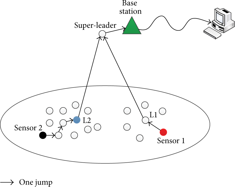
A WSN is a particular distributed system. On the basis of its working, all the needed communications concern the transfer of the collected environmental values from the sensors to the sink. As in the general case, the sink and the sensors are remote, and this communication is performed in several jumps. Partitioning in WSN consists of optimizing the number of jumps in the routing between any sensor and the sink. As the routing is closely dependent on the network organization, and organization in clusters has been commonly selected as the best to ensure the optimal routing, we propose in this paper a clustering algorithm that reduces as much as possible the number of jumps between any sensor and the sink (Figure 2).

Figure 2

The network before clustering.

2.5. Related Works

Organizing a system in clusters consists of putting together some objects, materials, or machinery in groups. The cluster concept allows for defining a group of entities as a single virtual entity: it assigns the same name to each member of a particular group and communicates with them using the same address. In each cluster, one member plays a particular role and is called leader, manager, interconnection point, or local coordinator. This one is responsible for communication between various members or levels, receiving information and referring to the other members, and overseeing the internal organization of the cluster. The notion of cluster can be extended by the definition of several-level hierarchy structure. A two-level hierarchy structure requires, in addition to clusters formation and the choice of a coordinator for each group, the election of an overall coordinator that is called global coordinator or super-leader, playing the role of interconnection point of all clusters. Many clustering algorithms have been conceived, widely studied, and classified. These algorithms are performed on the basis of specific metrics as, for instance, mobility [1, 8, 9], signal power [8], node weight [1, 8], density [9], distance between nodes [10], and the highest identifier [11]. The clustering improves the performance of dynamicity and scalability when the network size is important with high mobility. All of the characteristics and constraints imposed by sensors make the design of an efficient scheme for the self-organisation of WSN a real challenge. Before the design of our approach, a deep study of a big number of clustering protocols was conducted. Some of the studied protocols were conceived for ad hoc networks in general, while others were especially designed for WSN.

Heinzelman et al. (2000) [12] propose LEACH, which is a distributed, single hop clustering algorithm for homogeneous WSN. In LEACH, the cluster-head role is periodically rotated among the sensor nodes to evenly distribute energy dissipation. To implement this protocol, the authors assume that all sensors support different MAC protocols and perform long distance transmissions to the base station.

Reference [13] demonstrates a hierarchical routing protocol design (ECP) that can conserve significant energy in its setup phase as well as during its steady state data dissemination phase. ECP achieves clustering and routing in a distributed manner and thus provides good scalability. The protocol is divided into 3 phases: clustering, route management, and data dissemination.

Reference [14] proposes structuring nodes in zones. It aims to reduce the global view of the network to a local one. The author presents a distributed and low-cost topology construction algorithm, addressing the following issues: large-scale, random network deployment, energy efficiency, and small overhead.

Reference [15] proposes a stable and low-maintenance clustering scheme (NSLOC) that simultaneously aims to provide network stability combined with a low cluster maintenance cost.

Reference [1] proposes CSOS which is a strong weight-based clustering algorithm that consists of grouping sensors into a set of disconnected clusters, hence giving to the network a hierarchical organisation. Each cluster has a cluster-head that is elected among its 2-hop neighbourhood based on nodes weight. The weight of each sensor is a combination of 2-density, residual energy, and mobility. The use of the 2-density allows for generating homogeneous clusters and favoring the node that has the most related 2-neighbours to become cluster-head. The 2-density of a node u is the ratio of the number of links in its 2-neighbourhood (links between u and its neighbours and links between 2-neighbours of u) to the number of nodes in the 2-neighbourhood. CSOS takes place according to the following stages: leaders election followed by setup and reaffiliation stages for group formation.

Reference [16] proposes HSL-2-AN which is a simple approach that allows for organizing an ad hoc network into a two-level tree structure: several groups with a leader per group and a super-leader for the entire network. It takes place according to three stages: group formation, leader election, and finally the super-leader election. Groups are formed on the basis of a geographical metric, expressed by the distance between two nodes and the node scope. In each group, a leader is elected. The group leader is the node with the average distance between it and other group nodes being minimal. This reflects the fact that the leader should be close to the maximum of nodes in the group. The super-leader is the network node that has the maximum of leaders in its scope. Between the same group members, communication passes through the leader. Between different group members, communication passes through the coordinator. HSL-2-AN includes three parameters, baptised cohesion parameters to measure connectivity in the network. The use of these parameters is based on threshold values defined for each application. Three situations were identified and considered significant for the network: cohesion, strong cohesion, and absolute cohesion. The latter refers to the state in which communication is optimal.

Reference [2] presents an algorithm using a metric called k-density as a cluster-head selection criterion. This density is calculated using the number of neighbors, as well as the number of nodes of the two neighborhoods. The study in [17] showed that it requires a large number of messages. However, this is one criterion which makes the network more tolerant to the changes of the network topology. When a node moves, the cluster structure is not necessarily affected.

Reference [18] presents an energy constrained minimum dominating set based efficient clustering called ECDS which models the problem of optimality by the choice of cluster-heads with energy constraints. Three extensions of ECDS are presented by the authors: sECDS, kECDS, and mECDS. sECDS improves the performance of ECDS by introducing the rounded span which allows a larger cluster-head selection during each round of the algorithm. kECDS (k-hop cluster ECDS) extends the ECDS algorithm to clusters where a node can be up to k hops from its cluster-head. The last algorithm mECDS extends ECDS to be used with a multipath routing protocol. This version of the algorithm allows a node to choose up to m cluster-heads, which provides robustness by enabling multipath routing. With mECDS, multipath routing can be used not only from the cluster-head to the base station, but also from the node to one or more cluster-heads.

Reference [19] presents a new cluster-based protocol for WSN named ECLEACH. ECLEACH is a threshold-based protocol that selects the CHs based on their residual energy, their distance to other sensor nodes, and the residual energy of the other SNs. ECLEACH also keeps a minimum distance between every cluster-head and the next in order to have a better distribution of cluster-heads over the network. The evaluation shows that ECLEACH outperforms LEACH in terms of first node death time and average residual energy.

Reference [20] proposed a middleware called event-driven network controller (ENC) that is responsible for clustering multimodal sensor nodes only in the spacetime vicinity of a moving object and improving the data fusion. The ENC is energy-aware and also is able to improve the quality of data fusion by clustering only the sensors in the immediate vicinity of an event and moving sensors to better observe events. The ENC considers only one-hop clusters. In order to save energy, the sensor nodes may reduce their transmission power which may require them to form multihop clusters in order to group enough sensors of various modalities. ENC has been successfully applied to localize and track a Seg-way via the language-theoretic approach for multimodal sensor data fusion. Achievements showed that multimodal clustering is more robust to the environmental changes than single-modal clustering. The ENC middleware is generic and can be used in other applications as long as the notions of subpattern and pattern are defined.

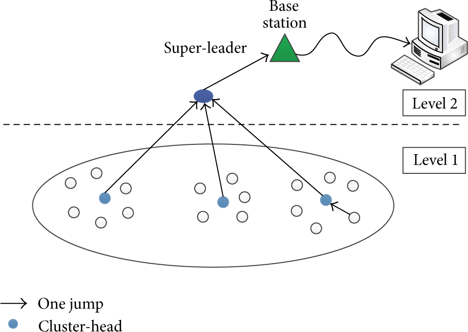
3. WSN-2-LTS (A WSN Two-Level Tree Structure)

In this section, we propose a new clustering algorithm that consists of grouping sensors into a set of disconnected clusters. The target structure is the two-level tree structure that consists of several clusters with a cluster-head per cluster in the level one and a super-leader node for the entire network in the level two.

The choice of this structure is driven by the insufficiency of the one-level hierarchy structures: The majority of the structures selected in ad hoc and sensor networks are one-level hierarchical, that is, multiple clusters with election of a cluster-head in each cluster; this structure has been extensively tested with different metrics for the selection of various members playing a role in the network. When using this structure, it is as if we reduce the number of network nodes. Because we assimilate all the cluster nodes to a single node that is the cluster-head of the cluster, we know that communication, decision making, and data exchange are done through the cluster-head, and the other members of the cluster are transparent to other network members. Level one structure improves the quality of service, but the problem remains, if the number of clusters grows a lot in increasing the number of nodes. The aim is to find efficient and automatically extensible frameworks, according to the number of nodes. Regarding our choice, we point out that our long-term goal is the n level hierarchy structure, with n being any and easily extensible. The choice of n depends on the number of nodes (sensors) and the number of base stations that are involved in the experimental platform. With the test of the two-level hierarchy structure, we create a basic structure we try to extend to determine hierarchical structures with higher levels (Figure 4).

Our algorithm is performed on the basis of some assumptions that we expose in the following paragraph.

3.1. Assumptions

• (1)

Network nodes constitute a related graph.

(2)

Communications are bidirectional and FIFO.

(3)

Messages arrive to destination at the end of a finite time.

(4)

Each node has some properties: energy quantity, signal power, mobility, and resources quantity.

(5)

We assume that each message is identified by a type which allows the recipient to treat it appropriately. Messages are numbered from 0 to 9.

(6)

The network is sufficiently stable during the clustering protocol execution.

(7)

Each node knows the coordinates of its neighbours. Particularly, each node knows if it is in the range of the sink or not.

3.2. The Metric Used for Cluster-Head Election

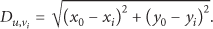
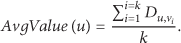
Let us note u as a node and $N_{\mathrm{1}}(u)$ as the neighborhood of u, that is, the set of neighbors of u. We define $AvgValue(u)$ as the average value of the distances between u and its neighbours (the nodes belonging to $N_{\mathrm{1}}(u)$ ). The cluster-head is the node v with $AvgValue(v)$ minimal. To calculate $AvgValue(u)$ , let us suppose $u(x_{\mathrm{0}},y_{\mathrm{0}})$ as a node, where $x_{\mathrm{0}}$ and $y_{\mathrm{0}}$ are its coordinates, and $N_{\mathrm{1}}(u)$ as the set of neighbors of u, composed of k nodes $v_{\mathrm{1}}(x_{\mathrm{1}},y_{\mathrm{1}}),v_{\mathrm{2}}(x_{\mathrm{2}},y_{\mathrm{2}}),\dots ,v_k(x_k,y_k)$ . The distance $D_{u,v_i}$ between $u(x_{\mathrm{0}},y_{\mathrm{0}})$ and any node $v_i(x_i,y_i)$ , $i\in \mathrm{1},\dots ,k$ is given by the formula:

$$\begin{array}{cc}& D_{u,v_i}=\sqrt{{\left(x_{\mathrm{0}}-x_i\right)}^{\mathrm{2}}+{\left(y_{\mathrm{0}}-y_i\right)}^{\mathrm{2}}}.\end{array}$$

(2)

And $AvgValue(u)$ is given by the formula:

$$\begin{array}{cc}& AvgValue\left(u\right)=\frac{{\sum }_{i=\mathrm{1}}^{i=k}{D}_{u,v_i}}{k}.\end{array}$$

(3)

3.3. Clusters Formation Principle

Since cluster-head is responsible for coordinating the cluster members, we proposed to set up periodically cluster-head election process not to exhaust its battery power. Moreover, for better management of the formed clusters, cluster formation takes into account the following constraints: each cluster has a size ranging between two thresholds $LimitSup$ and $LimitInf$ except in certain cases in which its value can be lower than $LimitInf$ . If, during configuration phase, there is formation of clusters whose size is lower than $LimitInf$ , reaffiliation process will be triggered. In our approach, we tried to organize sensors into clusters by affiliating each sensor to the nearest cluster-head from it. We used Hello messages for cluster formation in order to minimize broadcast overhead and not to degrade the algorithm of its performance. Hence, at the beginning, each sensor calculates its $AvgValue$ and generates a Hello message, which includes two extra fields, in addition to other regular contents, $AvgValue$ and $NodeCH$ , where $NodeCH$ is set to zero. Furthermore, clustering process is performed in two consecutive phases and clusters are formed one after the other. To establish a two-level tree structure, the third phase which consists of a super-leader election is followed.

3.4. Main Data Structures

• (1)

StateVector

 

It identifies the node, and its structure is $NodeId$ , $NodeCH$ , $State$ , $AvgValue$ , and $Size$ , where

 

$NodeId$ is the sensor's identifier,

 

$NodeCH$ is the sensor's cluster-head identifier (if this node is a cluster-head, then its identifier will be assigned to $NodeCH$ ),

 

$State$ is the sensor's state (L: leader, M: simple member, S: super-leader, and C: connection node),

 

$Size$ is the size of the cluster to which it belongs.

(2)

TableCluster

 

Each node is responsible for maintaining a table called “TableCluster,” in which the information of the local members of the cluster is stored. The format of this table is defined as TableCluster ( $NodeId$ , $NodeCH$ , $AvgValue$ ,   and   $nblead$ ), where $nblead$ is the number of leaders in the range of the sensor.

(3)

TableCH

 

Each cluster-head maintains a table, TableCH, in which the information about the other cluster-heads is stored. The format of this table is represented as $TableCH(NodeCH,AvgValue)$ .

(4)

ListeLeader

 

A list data structure is maintained by each node and stores identifiers of the leaders that are in the range of the node during the third phase of the algorithm.

3.5. List of Exchanged Messages

Table 1 shows the role of the used messages, and Figure 3 shows their structures where we represent only information pertinent to the step of the algorithm.

Table 1

Desciption of exchanged messages.

Identifier	Description and role
HelloElectLeader	Leader election
AdvJoin	Request for affiliation
ReqJoin	Affiliation request
AcceptJoin	Acceptance of affiliation
AdvReaff	Request for reaffiliation
ReqReaff	Reaffiliation request
AcceptReaff	Acceptation of reaffiliation
HelloElecConnect	Determination of connection nodes
InfNewState	Connection nodes inform their leaders about their new state
SentPsl	Sent by each leader of the provisional super-leader identifier in its cluster to the other leaders

Figure 3

Structures of messages.

Figure 4

Formed groups by WSN-2-LTS (number of nodes = 30).

3.6. WSN-2-LTS Pseudocode

WSN-2-LTS pseudocode is the composition of three stages: phase 1, phase 2, and phase 3 as shown in Algorithm 1. Phase 1, phase 2, and phase 3 are detailed and well commented, respectively, in Algorithms 2, 3, and 4.

Algorithm 1: WSN-2-LTS.

Begin

(1) Phase 1; # Algorithm 1 #

(2) Phase 2; # Algorithm 2 #

(3) Phase 3; # Algorithm 3 #

End

Algorithm 2: Phase 1.

Begin

(1) # This phase concerns the selection of cluster-heads and the configuration of the clusters #

(2) # ================================ #

(3) # Necessary Initializations #

(4) Initialize $$TimeCluster$$ ;

(5) # $$TimeCluster$$ is the time it takes for the execution of phase 1 #

(6) for  each node $$u\in G$$   do

(7)   $$u\to nodeId=NodeId$$

(8)   $$u\to NodeCH=\mathrm{0}$$

(9)   $$u\to Size=\mathrm{0}$$

(10)    $$u\to State$$  = ‘M’  # Initially all the nodes are simple members #

(11) end for

(12) # Each node $$u\in G$$ calculates its $$AvgValue$$ #

(13) for  each node $$u\in G$$     do

(14)   u calculates $$AvgValue(u)$$

(15) end for

(16) # Election of leaders #

(17) # each node broadcasts $$HelloElectLeader$$ to its neighbors #

(18) # the node with the lowest $$AvgValue$$ is selected $$CH$$ #

(19) Select $$v\in N_{\mathrm{1}}\left[u\right]:$$

(20) $$AvgValue\left[v\right]=(max\left(AvgValue\left(w\right):w\in N_{\mathrm{1}}\left[u\right]\right)$$

(21)   $$UpdateStateVect(CH)$$   ⊳ update of $$CH$$ State Vector

(22)   $$CH\to nodeCH=CH\to nodeId$$

(23)   $$CH\to Size=\mathrm{1}$$

(24)   $$CH\to State=$$  ‘L’

(25)  # Configuration of the clusters #

(26) repeat

(27)    $$CH$$ sends $$AdvJoin$$ to $$N_{\mathrm{1}}(CH)$$

(28)   if  ( $$u\in N_{\mathrm{1}}(CH)$$ receives $$advJoin$$ )  and  ( $$u\to NodeCH=\mathrm{0}$$ )  and

       ( $$AvgValue[u]<AvgValue[CH]$$ )  then

(29)    # request for affiliation #

(30)    u sends a $$ReqJoin$$ to $$CH$$

(31)    # $$CH$$ verifies if the size of its cluster does not reach $$LimitSup$$ #

(32)    if   $$CH\to Size<LimitSup$$   then

(33)      $$CH$$ sends $$AcceptJoin$$ to u

(34)     # $$CH$$ performs the accession procedure #

(35)      $$CH\to Size=CH\to Size+\mathrm{1}$$

(36)     # u performs the accession procedure #

(37)      $$u\to NodeCH=CH\to NodeCH$$

(38)      $$u\to Size=CH\to Size$$

(39)    end if

(40)   end if

(41)   Update( $$TableCluster$$ )

(42) until  expired( $$TimeCluster$$ )

End

Algorithm 3: Phase 2.

Begin

(1) # This phase concerns the re-affiliation process #

(2) # ============================ #

(3) # each CH with a cluster size < LimitSup

  performs the following treatment #

(4) if   $$CH\to Size<LimitSup$$   then

(5)    $$CH$$ sends $$AdvReaff$$ to $$N_{\mathrm{1}}(CH)$$

(6)   if  ( $$u\in N_{\mathrm{1}}(CH)$$ receives $$\mathrm{A}dvReaff$$ )  and

     ( $$u\to Size$$ < $$LimitInf$$ )  and  

    ( $$AvgValue(u)$$ < $$AvgValue(CH)$$ )  then

(7)    u sends $$ReqReaff$$ to the nearest $$CH$$

(8)    if   $$CH\to Size<LimitSup$$   then

(9)      $$CH$$ sends $$AcceptReaff$$ to u

(10)     # $$CH$$ updates its State Vector #

(11)      $$CH\to Size=CH\to Size+\mathrm{1}$$

(12)     # u updates its state vector #

(13)      $$u\to Nod{e}_{CH}=CH\to Nod{e}_{CH}$$

(14)      $$u\to Size=CH\to Size$$

(15)    end if

(16)   end if

(17) end if

(18) Update( $$TableCluster$$ )

End

Algorithm 4: Phase 3.

Begin

(1) # This phase concerns the determination of connection

  nodes and the election of the super-leader #

(2) # ================================ #

(3) # Determination of connection nodes #

(4) each node u broadcasts in $$N_{\mathrm{1}}(u)$$    $$HelloElecConnect$$

(5) each node v receiving at least one $$HelloElecConnect$$

(6) from a node belonging to another cluster,

  is a connection node

(7) v updates its $$StateVector$$

(8) $$v\to state=$$  ‘C’

(9) v sends to its leader $$InfNewState$$

(10) # $$InfNewState$$ indicates the number of leaders $$\in N_1(v)$$

   and if v is in the range of the sink or not #

(11) # $$Super\text{-}leader$$ selection #

(12) # The $$super\text{-}leader$$ is the node in the range of the sink,

   and with the maximum of leaders in its range #

(13) From $$InfNewState$$ each $$C{H}_k$$ selects the provisional

   $$super\text{-}leader$$    $$PS{L}_k$$ in the cluster number k

(14) $$C{H}_k$$ sends $$SentPsl$$ to other leaders via connection

  nodes

(15) Each leader selects the network $$super\text{-}leader$$    $$SL$$

(16) $$SL\to state=$$  ‘S’

End

3.7. Communication and Routing

In normal operation (no failures or stop), we propose in our structure that values collected by sensors follow the following path to reach the sink.

• (1)

In each cluster, each sensor sends its parameters to its leader.

(2)

Each leader applies to these settings an aggregation function Lead_AGR_Func() which depends on the application.

(3)

Via connection nodes, each leader sends the aggregated data to the super-leader.

(4)

The super-leader applies an aggregation function SLead_AGR_Func() to the data coming from all leaders and then sends the resulting data to the sink.

3.7.1. Aggregation Functions

The aggregation functions Lead_AGR_Func() and SLead_AGR_Func() generally depend on the application and may be identical or different. In the simplest case min, max, or average is used [21]. In the general case, an aggregation function may be a calculation, a filtering, or a compression and eventually the composition of the three operations.

4. Cohesion Parameters and Reorganization Strategy

4.1. Cohesion Parameters

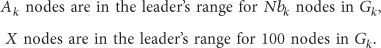
We use three factors [22] to measure our structure performance: the group cohesion factor $\text{Group}\_\text{cohesio}{\text{n}}_k$ as the percentage of nodes in coverage field of their leader in the group number k ( $G_k$ ), the network cohesion factor Network_Cohesion as the percentage of leaders in the coverage field of the super-leader, and Taux_group_cohesion as the percentage of groups in cohesion. According to these definitions, the group_cohesion factor has a different value in each group, but each of Network_Cohesion and Taux_group_cohesion factors is calculated for the whole network. In order to define these parameters, let us suppose $A_k$ , B, C, $N{b}_k$ , and NBG are as follows:

•  

$A_k$ = number of members that are in the range of the leader in $G_k$ ,

 

$N{b}_k$ = the number of nodes in $G_k$ ,

 

B = number of leaders that are in the range of the super-leader,

 

C = number of groups that are in cohesion,

 

NBG = the number of groups (or leaders) in the network.

We may write

$$\begin{array}{cc}& \text{Group}\_\text{cohesio}{\text{n}}_k=\frac{A_k}{N{b}_k}·\mathrm{100},\\ \text{Network}\_\text{Cohesion}=\frac{B}{\text{NBG}}·\mathrm{100},\\ \text{Taux}\_\text{group}\_\text{cohesion}=\frac{C}{\text{NBG}}·\mathrm{100}.\end{array}$$

(4)

The previous formulas are obtained by applying the rule of three. For instance, to calculate $\text{Group}\_\text{cohesio}{\text{n}}_k$ ,

$$\begin{array}{cc}& A_k\mathrm{\hspace{0.17em}\hspace{0.17em}}\text{nodes}\mathrm{\hspace{0.17em}\hspace{0.17em}}\text{are}\mathrm{\hspace{0.17em}\hspace{0.17em}}\text{in}\mathrm{\hspace{0.17em}\hspace{0.17em}}\text{the}\mathrm{\hspace{0.17em}\hspace{0.17em}}\text{leader's}\mathrm{\hspace{0.17em}\hspace{0.17em}}\text{range}\mathrm{\hspace{0.17em}\hspace{0.17em}}\text{for}\hspace{0.17em}\hspace{0.17em}N{b}_k\mathrm{\hspace{0.17em}\hspace{0.17em}}\text{nodes}\mathrm{\hspace{0.17em}\hspace{0.17em}}\text{in}\mathrm{\hspace{0.17em}\hspace{0.17em}}{G}_k,\\ X\mathrm{\hspace{0.17em}\hspace{0.17em}}\text{nodes}\mathrm{\hspace{0.17em}\hspace{0.17em}}\text{are}\mathrm{\hspace{0.17em}\hspace{0.17em}}\text{in}\mathrm{\hspace{0.17em}\hspace{0.17em}}\text{the}\mathrm{\hspace{0.17em}\hspace{0.17em}}\text{leader's}\mathrm{\hspace{0.17em}\hspace{0.17em}}\text{range}\mathrm{\hspace{0.17em}\hspace{0.17em}}\text{for}\mathrm{\hspace{0.17em}\hspace{0.17em}}\mathrm{100}\mathrm{\hspace{0.17em}\hspace{0.17em}}\text{nodes}\mathrm{\hspace{0.17em}\hspace{0.17em}}\text{in}\mathrm{\hspace{0.17em}\hspace{0.17em}}{G}_k.\end{array}$$

(5)

Therefore,

$$\begin{array}{cc}& X=\frac{A_k}{N{b}_k}·\mathrm{100}\mathrm{\hspace{0.17em}\hspace{0.17em}}\text{nodes}=\text{Group}\_\text{cohesio}{\text{n}}_k.\end{array}$$

(6)

In the same way, $\text{Network}\_\text{cohesion}$ and $\text{Taux}\_\text{group}\_\text{cohesion}$ are calculated.

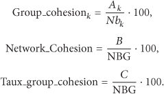
Let us suppose that SGC, SNC, and STGC are, respectively, Group_cohesion, Network_Cohesion, and Taux_Group_Cohesion thresholds. At any time, these parameters can be calculated. We retain three different cases for these parameters as meaningful cases for the network that are as follows:

• (1)

Cohesion, if

 

Taux_group_cohesion ≥ STGC and Network_Cohesion ≥ SNC.

 

This situation corresponds to the fact that the majority of the group members are in their leader's range and the majority of the leaders are in the super-leaders' range (Figure 5).

(2)

Strong cohesion, if

• (i)

Taux_group_cohesion = 100 (with SGC = 100 in all the groups) and Network_Cohesion > SNC.

 

This means that all groups members are in the range of their leaders, and the majority of the leaders are in the super-leaders' range (Figure 6).

(ii)

Taux_group_cohesion = 100 (with SGC ≤ group_cohesion < 100 in all the groups) and Network_Cohesion = 100.

 

This implies that, in each group, the majority of the members are in the range of their leader, and in the network all the leaders are in the range of the super-leader (Figure 7).

(3)

Absolute cohesion, if

 

Network_Cohesion = 100 and Group_cohesion = 100 for each of the network groups.

 

All leaders are in the super-leader's range, and the members of each group are in their leader's range (Figure 8).

Figure 5

One case of the cohesion state.

Figure 6

Case one of strong cohesion.

Figure 7

Case two of strong cohesion.

Figure 8

The case of absolute cohesion.

4.2. Reorganization Strategy

Initially, at the end of the organization process, the $\text{Group}\_\text{cohesion}$ value in every group k is equal to 1, because all the clusters are formed in the one neighborhood. $\text{Network}\_\text{cohesion}$ and $\text{taux}\_\text{group}\_\text{cohesion}$ are equal to their initial values, respectively, $\text{Init}\_\text{Network}\_\text{cohesion}$ and $\text{Init}\_\text{taux}\_\text{group}\_\text{cohesion}$ . With the change of the network topology caused by the nodes mobility these values may change. Periodically, every group leader calculates the instantaneous $group\_cohesion$ value and sends it to the super-leader. This last calculates then $\text{Network}\_\text{cohesion}$ and $\text{taux}\_\text{group}\_\text{cohesion}$ . Note that the calculation of these values uses the number of instantaneous neighbours that may be known thanks to Hello messages that are sent periodically in the neighbourhood. The super-leader makes a comparison between these values and their thresholds and decides whether to broadcast the reorganization message or not. In the general case, where cohesion parameters do not change much, reorganisation is triggered periodically (period = T defined for each application).

5. The Relation between Cohesion Parameters and the Partitioning

Three states are defined for the network: cohesion, strong cohesion, and absolute cohesion.

• (1)

The Cohesion State

 

Some of the sensors are not in the range of their leaders and these leaders are not in the range of the super-leader. Hence, the packet performs several jumps from the sensor to its leader, several jumps from its leader to the super-leader, and then one jump to reach the sink. This case constitutes the worst situation in the network.

(2)

The Strong Cohesion State

• (i)

First Case

 

All the sensors are in the range of their leaders, and some of the leaders are not in the range of the super-leader. Hence, communication may be performed in one jump from the sensor to its leader, several jumps from its leader to the super-leader, and then one jump to reach the sink.

(ii)

Second Case

 

All the sensors are not in the range of their leaders, and all the leaders are in the range of the super-leader. Hence, communication may be held according to several jumps from the sensor to its leader, one jump from the leader to the super-leader, and then one jump to reach the sink.

(3)

The Absolute Cohesion State

 

All the sensors are in the range of their leaders and all the leaders are in the range of the super-leader. Hence, each packet performs one jump from the sensor to its leader, one jump from the leader to the super-leader, and a third jump to reach the sink. From the partitioning point of view, this state is the best for the network. In all, three jumps are needed to reach the sink from any sensor.

6. Simulation

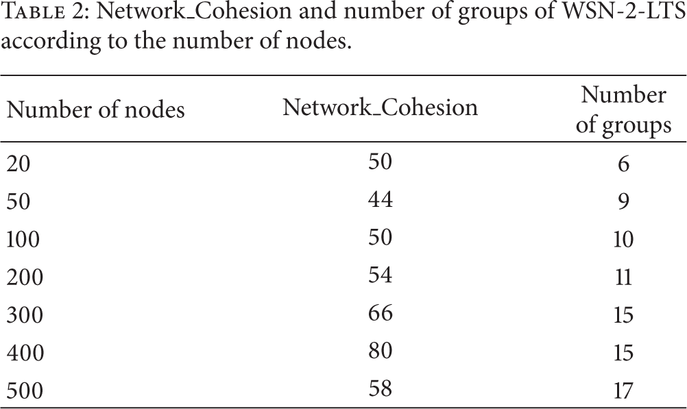
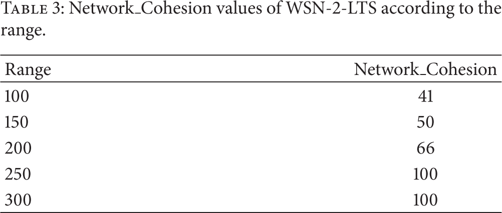
Several simulators exist to simulate the working of WSN [23]. In order to have simulation results of our algorithm, we used version 2.31 of the network simulator NS2. In the first step of our work we established some curves that concern the number of formed groups (Table 2 and Figure 9), Network_Cohesion (Tables 2 and 3 and Figures 10 and 11), and the running time (Table 4 and Figure 12).

Table 2

Network_Cohesion and number of groups of WSN-2-LTS according to the number of nodes.

Number of nodes	Network_Cohesion	Number of groups
20	50	6
50	44	9
100	50	10
200	54	11
300	66	15
400	80	15
500	58	17

Table 3

Network_Cohesion values of WSN-2-LTS according to the range.

Range	Network_Cohesion
100	41
150	50
200	66
250	100
300	100

Table 4

Running time of WSN-2-LTS according to the number of nodes.

Number of nodes	Running time
20	0
50	0
100	1
200	6
300	33
400	75
500	150

Figure 9

The number of formed groups according to the number of nodes.

Figure 10

Variation in Network_Cohesion according to the number of nodes.

Figure 11

Variation in Network_Cohesion according to the range.

Figure 12

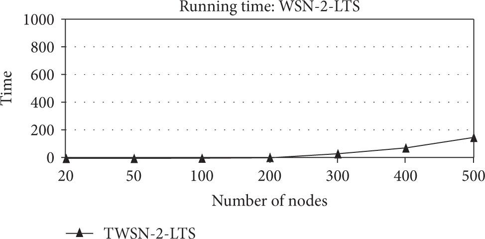
Running time of WSN-2-LTS.

The second step of our simulation concerns the comparison of WSN-2-LTS to CSOS [1] and HSL-2-AN [16], previously published protocols.

We studied the scalability of our approach and the repartition of the nodes within the formed clusters. We simulated the three algorithms for 20, 50, 100, 200, 300, 400, and 500 nodes and established a number of representative curves.

The approach of forming groups in CSOS is based on a very strong metric (weight) chosen for the leader election: the formula defining the weight is as follows:

$$\begin{array}{cc}& \text{weight}\left(u\right)=\alpha \mathrm{\ast }{P}_{\mathrm{2}\text{-density}}+\beta \mathrm{\ast }{P}_{\text{res}\_\text{energy}}+\gamma \mathrm{\ast }{P}_{\text{mobility}}\end{array}$$

(7)

such that

$$\begin{array}{cc}& \alpha +\beta +\gamma =\mathrm{1}.\end{array}$$

(8)

The strength of this metric lies in the fact that it takes into account three parameters at once, the geographical criterion, the remaining energy, and the node mobility. By varying the value of α, β, or γ we can increase, decrease, or cancel the importance of a criterion in the metric.

In HSL-2-AN approach, the group formation stage takes into account only the geographical criterion, which poses no constraint on the number of nodes. Hence, the resulting groups can be very different in number of nodes and may even be composed of a single node. This imbalance in the number of nodes per group leads to an unbalanced load in the network between groups and between nodes.

In the design of WSN-2-LTS, the leader election metric is similar to the metric used in HSL-2-AN. But the election itself and group formation are performed as in CSOS. The second stage of WSN-2-LTS is the determination of connection nodes in order to facilitate routing; then the super-leader election is followed on the basis of the same metric used in HSL-2-AN but it is performed in a different manner. Cohesion parameters are defined and discussed as in HSL-2-AN. A specific routing path is defined then to reach the sink (sensor, leader, Super-leader, and sink), with a data aggregation operation at the leaders and the super-leader nodes. Some measures were taken by simulation on the basis of different criteria: reaffiliation rate, number of formed groups, Network_Cohesion, and the balance of groups in a number of nodes.

Both CSOS and WSN-2-LTS use the reaffiliation technique; Figure 13 compares the reaffiliation rate in the two protocols. The rate of reaffiliation is higher in WSN-2-LTS because this one forms a larger number of clusters. This is due to the fact that WSN-2-LTS forms clusters in the one neighbourhood but CSOS forms clusters in the two neighbourhoods. Figure 13 and Table 5 illustrate obtained values.

Table 5

Reaffiliation rate values for WSN-2-LTS and CSOS according to number of nodes.

Number of nodes	CSOS	WSN-2-LTS
20	8	6
50	35	64
100	27	176
200	64	324
300	101	676
400	136	876
500	840	1384

Figure 13

Reaffiliation rate of CSOS and WSN-2-LTS.

Both HSL-2-AN and WSN-2-LTS define cohesion parameters; Figure 14 compares $\text{Network}\_\text{Cohesion}$ in the two protocols. Cohesion parameters are defined identically in the two protocols and their values depend strongly on the leader, the super-leader, and all the nodes positions. Note that the operation of clustering is made differently in the two protocols, and it is why the curves show different values of Network_Cohesion for the same number of nodes in the the two protocols. Figure 14 and Table 6 illustrate obtained results.

Table 6

Network_Cohesion values for WSN-2-LTS and HSL-2-AN according to number of nodes.

Number of nodes	HSL-2-AN	WSN-2-LTS
20	60	50
50	42	44
100	83	50
200	66	54
300	77	66
400	77	80
500	55	58

Figure 14

Network cohesion of WSN-2-LTS and HSL-2-AN.

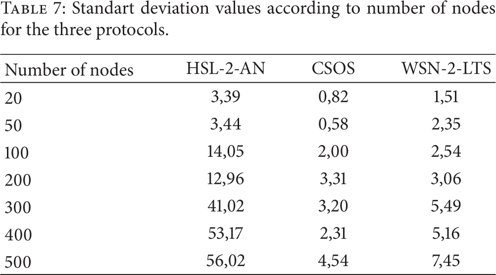
In order to study the balancing of the groups in terms of number of nodes we used the concept of standard deviation. The standard deviation is a mathematical quantity, widely used in statistics and informs us about the homogeneity of a set of discrete values: when the standard deviation of a set of values tends to zero, this means that the values are roughly equal. We calculated the standard deviation of the numbers of nodes in the different groups, for each number of nodes (20, 50, 100, 200, 300, 400, and 500) and for each of WSN-2-LTS, CSOS, and HSL-2-AN. We established then the curves shown in Figure 15 from Table 7.

Table 7

Standart deviation values according to number of nodes for the three protocols.

Number of nodes	HSL-2-AN	CSOS	WSN-2-LTS
20	3,39	0,82	1,51
50	3,44	0,58	2,35
100	14,05	2,00	2,54
200	12,96	3,31	3,06
300	41,02	3,20	5,49
400	53,17	2,31	5,16
500	56,02	4,54	7,45

Figure 15

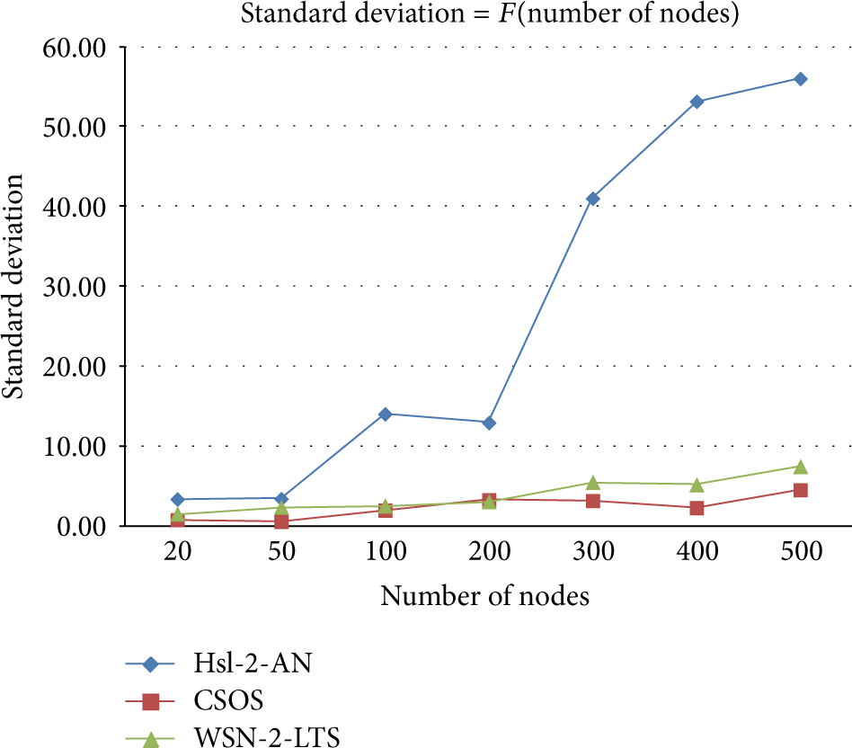
Balancing of the number of nodes in groups (WSN-2-LTS versus CSOS versus HSL-2-AN).

Let us suppose N is the number of formed groups and $x_{\mathrm{1}},\dots ,x_N$ , respectively, are the numbers of the nodes in the groups $G_{\mathrm{1}},\dots ,G_N$ .

The standard deviation $\text{SD}$ is given by the following formula:

$$\begin{array}{cc}& \text{SD}=\sqrt{\frac{{\sum }_{i=\mathrm{1}}^n{\left(x_i-\stackrel{-}{x}\right)}^{\mathrm{2}}}{N}},\end{array}$$

(9)

such that

$$\begin{array}{cc}& \stackrel{-}{x}=\frac{{\sum }_{i=\mathrm{1}}^n\left(x_i\right)}{N}.\end{array}$$

(10)

The less the standard deviation SD is, the more the number of nodes is balanced in all the groups.

Figure 15 and Table 7 show that, compared to HSL-2-AN, each of WSN-2-LTS and CSOS gives balanced groups.

7. Conclusion

Organizing in clusters has been judged as the best to optimize routing in ad hoc and wireless sensor networks. In this paper we presented a new clustering approach for partitioning in WSN. Our motivation is based on the fact that graph theory methods that are usually used to perform partitioning in wired networks are not applicable to WSN. This is due to their topology and the presence of multihop communication, a principle used by the sensors to send the captured data to the sink. As the routing depends on the network's organization, we proposed a two-level clustering algorithm to reduce as much as possible the number of jumps to reach the sink from any sensor. Our proposed organization consists of many clusters with one cluster-head per cluster in the first level and one super-leader for the entire network in the second level. To perform the evaluation of the algorithm and the validation of its performances, we introduced cohesion parameters. The proposed algorithm WSN-2-LTS has been applied to WSN with a range of nodes varying from 20 to 500. The presented simulation results show that the proposed algorithm provides better nodes cohesion against super-leader and sink. This cohesion certainly improves the information flows within the network and thus increases the energy autonomy. A suggestion for a future improvement for wsn-2-lts is to introduce other metrics such as weight metric in order to make the proposed protocol suitable for a big number of applications.