Scheduling and Power Control for Energy-Optimality of Low Duty Cycled Sensor Networks

Abstract

The main limitation of operating sensor networks autonomously is the finite battery capacity of sensor nodes. Sensors are usually operated at low duty cycle; that is, they remain in active mode for short duration of time, in order to prolong the network lifetime. However, operating at low duty cycle may result in significant performance degradation in system operation. Hence, in this work, we quantitatively investigate the tradeoff between the duty cyle and network performance. Specifically, we address the design of efficient channel access protocol, by developing a scheduling algorithm based on well known Lyapunov optimization framework. Our proposed policy dynamically schedules transmissions of sensor nodes and their sleep cycles by taking into account the time-varying channel state information, traffic arrivals, and energy consumptions due to switching between operational modes. We analytically show that our policy is energy optimal in the sense that it achieves an energy consumption which is arbitrarily close to the global minimum solution. We use simulations to confirm our results.

1. Introduction

Wireless sensor networks have the potential to improve the operations of conventional systems with the enhanced situational awareness that they can provide. There are many military, scientific, medical, or commercial applications of sensor networks currently in use. Sensor networks consist of battery operated sensor nodes performing sensing tasks and communicating their observations to a sensor fusion center. They are uniquely identified by the requirement of operation them for long periods of time without outside intervention. Hence, reducing the energy consumption of these devices is a primary concern. A common method to prolong network lifetime is to power down the sensor devices periodically. This type of operation provides significant savings in energy consumption at the cost of degrading the network performance.

The duty cycle of a node is defined as the proportion of time the node stays active in its lifetime [1]. When a sensor node is active, the energy is consumed by the radio, processing and sensing circuitry. When the node is in sleep mode, no current flows in most of the circuitry leading to significantly reduced energy consumption. However, depending on the design of the circuit of the sensor node, there may also be energy consumed while the node switches between active and idle modes and vice versa. For example, in [2] for  CC1010 type sensor nodes, while the switching energy from sleep mode to transmit mode is given as 47.75 μJ for the switching time which is 0.7 ms, the energy consumed during the transmission taken 0.7 ms is equal to 124.8 μJ.

In some important sensor applications, there are multiple data delivery tasks that must be performed by sensor nodes with low duty cycle. In these cases, severe transmission congestion and data loss may occur. In order to prevent the congestion and data loss, these tasks should be scheduled in an intelligent way. There is a plethora of work investigating opportunistic scheduling in different types of applications and networks. Examples of centralized and distributed scheduling algorithms that provide long term, temporal, throughput fairness guarantees and power control are addressed in [3–7]. Most of the prior works aim to stabilize a network with stochastic traffic by dynamically scheduling the nodes in the network based on the queue dynamics and instantaneous channel conditions. The seminal work by Tassiulas and Ephremides in [8] first introduced the design of backpressure algorithms based on Lyapunov drift techniques to achieve network stability and the authors in [9] developed algorithm which deals with performance optimization and queue stability problems simultaneously in a unified framework. There exists also a rich literature on using Lyapunov drift optimization for solving problems of energy optimization in wireless networks.

In this paper, we develop an energy optimal switching and scheduling (ESS) algorithm based on the Lyapunov drift framework for low duty cycle sensor networks. Our algorithm dynamically determines the operational mode of each sensor node, and it schedules a single node for transmission at each slot based on the energy consumption at each mode (i.e., sleep, active, and switching energy), channel conditions, and traffic load of nodes. We show that ESS algorithm is energy optimal in the sense that the overall expected energy consumption can be arbitrarily pushed to the global minimum energy with a tradeoff of an increase in average queue backlogs. In our simulations, we demonstrate that the proposed ESS algorithm prolongs the lifetime compared to the benchmark algorithms which do not take into account the energy cost of switching between different modes of operation.

2. Related Works

There has been significant works that aim to reduce the energy consumption of wireless networks, for example, [10–12]. In most prior works, the proposed algorithms have been designed by only taking into account the energy consumption in the active and sleep modes ignoring the effect of the consumed energy during switching from one mode to another. In addition, there is even fewer works on investigating the problem of stabilizing these networks while minimizing the total energy consumed. In particular, the opportunistic scheduling algorithms based on the one given in [8] that are employed to stabilize the network require the nodes to always have their radios turned on for polling and/or transmission. In [13], the authors proposed a suite of wireless sensor network protocols that take into account the source of energy consumptions in a network simulation model. In this work, the authors mentioned switching energy but leaved it as an open research problem. The study in [14] considered the switching energy cost, since it was observed that significant energy consumption occurs when switching from sleep mode to the active mode. On the other hand, in some studies like [15] it has been stated that the energy cost of switching is small. Generally, it is common to ignore switching energy in the literature. There are also various approaches proposed for designing duty cycling protocols [2, 16, 17], for sleep mode protocols [18] and for routing protocols [19, 20]. In [21], the authors aim to improve the end-to-end delay performance of sensor nodes by assuming that nodes operate in a periodic sleep schedule. A Carrier Sense Multiple Access/Collision Avoidance (CSMA/CA) based MAC algorithm is developed in [22] by taking into account the traffic condition of nodes. All of these works try to maximize the lifespan or the utility of the network without considering the network stability problem.

The works in [23–26] are the most important ones considering network stability issue for wireless sensor network. In [23], the authors proposed a back pressure algorithm designed using a Lyapunov drift based optimization framework using the receiver capacity model. However, the authors did not aim to minimize the average energy consumption. An optimal control algorithm for rechargeable wireless sensor nodes is proposed in [24] where the objective function maximizes the network utility subject to stability. In [25], the authors proposed a scheduling algorithm based on Lyapunov optimization theory in order to minimize the energy consumed while maintaining the network stability. However, their work does not apply to low duty cycle sensor networks. The network stability is studied in [26] for low duty cycle sensor networks. In this work, however, the authors do not take into account the switching energy.

In this paper, we develop a throughput optimal scheduling algorithm based on the Lyapunov drift framework which not only minimizes the energy consumed but also stabilizes the network of queues in a low duty cycle sensor network. Our energy-based switching and scheduling (ESS) algorithm is shown to be energy optimal in the sense that it minimizes the overall expected energy consumed in the network over all scheduling algorithms and it remains throughput optimal. The proposed ESS algorithm prolongs the lifetime compared to a benchmark algorithm which does not consider the switching energy cost.

3. System Model and Problem Statement

3.1. System Model

We consider a sensor network where N sensor nodes sense the environment and transmit information to a sink node in a single-hop fashion. This type of WSN is very common in practice where each sensor has a different task and these tasks must be managed at a centralized system. We consider a time-slotted system where the time slot is the resource to be shared among different nodes. We adopt a noninterference model where only one node is receiving data at any given time. Random channel gains between base station and other nodes in the network are assumed to be independent and identically distributed (iid) over time according to a general distribution, and they are independent across nodes with values taken from a finite set. Moreover, we assume that channel gains are time-varying but fixed over the time slot duration. The data rate of node n during slot t is represented by ${\mu }_n(I_n(t),g_n(t))$ (in units of packets/slot) where $g_n(t)$ is the channel state of node n and $I_n(t)=\mathrm{1}$ , whenever node n is selected as a transmitting node at time t, and $I_n(t)=\mathrm{0}$ otherwise. We assume that ${\mu }_n(I_n(t),g_n(t))$ is upper bounded with ${\mu }_n(I_n(t),g_n(t))\le {\mu }_{\max }$ . For ease of exposition, we use ${\mu }_n(t)$ instead of ${\mu }_n(I_n(t),g_n(t))$ in the rest of the paper.

Each sensor node has a separate queue. Packets arrive into its queue according to a stationary arrival process that is independent across users and time slots. Let $A_n(t)$ be the amount of data arriving into the queue of user n at time slot t. Let $\mathbf{Q}(t)=(Q_{\mathrm{1}}(t),Q_{\mathrm{2}}(t),\dots ,Q_N(t))$ denote the queue length vector. The dynamics of queue length for node n is given as

$$\begin{array}{cc}& Q_n(t+\mathrm{1})={\left[Q_n\left(t\right)+A_n\left(t\right)-{\mu }_n\left(t\right)\right]}^{+},\end{array}$$

(1)

where $[x{]}^{+}=\max (x,\mathrm{0})$ . We define the network admission rate vector as $\mathbf{\lambda }=\{{\lambda }_{\mathrm{1}},{\lambda }_{\mathrm{2}},\dots ,{\lambda }_N\}$ where ${\lambda }_n$ is the average exogenous arrival rate of node n. Let Λ be the network capacity region, that is, the set of all feasible admission rate vectors that the network can support.

In our network model, a sensor node can be either in active or sleep mode during a time slot. We denote $\mathcal{N}$ as the set of all nodes in the network. We also denote z as energy mode of sensor node, where $z=\mathrm{0}$ and $z=\mathrm{1}$ represent the sleep and active modes, respectively. The sensor can also switch from active to sleep or vice versa and we denote $s\in \{\mathrm{01,10}\}$ as the switching action where $s=\mathrm{01}$ and $s=\mathrm{10}$ represent the switching from sleep to active and active to sleep modes, respectively. In addition, we denote the set of all sleep and active nodes as $\mathcal{S}(t)$ and $\mathcal{A}(t)$ at time t, respectively, and $\mathcal{S}(t)\cup \mathcal{A}(t)=\mathcal{N}$ .

3.2. Problem Formulation

We say that a queue is strongly stable if

$$\begin{array}{cc}& \underset{t\to \infty }{\mathrm{limsup}}\frac{\mathrm{1}}{t}{\displaystyle \sum }_{\tau =\mathrm{0}}^{t-\mathrm{1}}‍\mathbb{E}\left(Q_n\left(t\right)\right)<\infty .\end{array}$$

(2)

Moreover, if every queue in the network is stable, then the network is called stable. The stability region of the network is the the closure of the convex hull of all arrival rate points for which there exists a feasible scheduling policy that stabilizes the network [9].

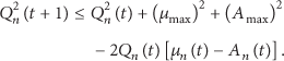
We consider an energy consumption model defined as follows. At the beginning of transmission, each sensor has a full battery of $E_{\text{tot}}$ . In each time slot, a particular node can be in either active or sleep modes according to its remaining energy, queue backlog, and channel condition. During the sleep mode, the node is unable to transmit packets. However, packets continue to be generated by the node, and they are queued until the node has the opportunity to transmit them. Let $E_n^z(t)$ be the energy consumed by node n when it is in mode $z\in \{\mathrm{0,1}\}$ at time t. When the node is active, it consumes an energy $c_n(t)$ that depends on the current draw of active mode by the circuit and how much time the node spends in active mode. Also, the energy needed for packets transmission should be included to the total energy expenditure when the node is selected to transmit. Then at time t, the total energy consumption by node n in active mode becomes $E_n^{\mathrm{1}}(t)=c_n(t)+{\mu }_n(t){\alpha }_n$ where ${\alpha }_n$ denotes the energy spent for a packet transmission. Furthermore, if a node switches from sleep-to-active or active-to-sleep modes, then the switching energy denoted as $E_n^s(t)$ is consumed. The values of energy costs are given in Section 6. Hence, the overall energy spent by node n during time slot t is given by

$$\begin{array}{cc}& H_n\left(t\right)={\displaystyle \sum }_{z=\mathrm{0}}^{\mathrm{1}}‍E_n^z\left(t\right)+E_n^s\left(t\right).\end{array}$$

(3)

The total energy consumption in the network at time slot t is obtained by summing over all nodes in the system:

$$\begin{array}{cc}& H\left(t\right)={\displaystyle \sum }_{n=\mathrm{1}}^N‍{\displaystyle \sum }_{z=\mathrm{0}}^{\mathrm{1}}‍E_n^z\left(t\right)+{\displaystyle \sum }_{n=\mathrm{1}}^N‍E_n^s\left(t\right).\end{array}$$

(4)

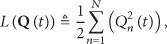
Define the time average expected total energy consumption as

$$\begin{array}{cc}& \overline{H}=\underset{t\to \infty }{\mathrm{limsup}}\frac{\mathrm{1}}{t}{\displaystyle \sum }_{\tau =\mathrm{0}}^{t-\mathrm{1}}‍\mathbb{E}\left[{\displaystyle \sum }_{n=\mathrm{1}}^N‍{\displaystyle \sum }_{z=\mathrm{0}}^{\mathrm{1}}‍E_n^z\left(\tau \right)+{\displaystyle \sum }_{n=\mathrm{1}}^N‍E_n^s\left(\tau \right)\right].\end{array}$$

(5)

The expectation is with respect to the randomness that arises from channel variations and arrival process and possibly from random stationary switching policy. The overall energy consumption during time t is upper bounded by a finite value since all sensors have a limited battery power and thus, without loss of generality, we assume that the following is satisfied at every time slot:

$$\begin{array}{cc}& {\displaystyle \sum }_{n=\mathrm{1}}^N‍H_n\left(t\right)\le H_{\max },\hspace{1em}\forall t.\end{array}$$

(6)

We are interested in minimizing the total average energy consumption in the network while keeping the queue sizes of the sensor nodes bounded. Then, our optimization problem can be formalized as follows:

$$\begin{array}{l}\min \hspace{1em}\overline{H}\\ \text{s}.\text{t}.\hspace{1em}\text{network}\hspace{0.17em}\hspace{0.17em}\text{stability}.\end{array}$$

(7)

4. Energy-Aware Switching and Scheduling (ESS) Algorithm

In this section, we introduce our energy-aware sleep-active scheduling algorithm which asymptotically minimizes the average network energy consumption subject to the network stability. Furthermore, the proposed algorithm is shown to be throughput optimal; that is, the algorithm can guarantee the network stability for all feasible network admission rates.

At each time slot, the proposed energy-aware switching and scheduling (ESS) algorithm determines the energy modes of operation for each sensor nodes and selects the transmitting node which maximizes the following:

ESS:

$$\begin{array}{cc}& \underset{n\in \mathcal{A}}{\max }\mathrm{\hspace{0.17em}\hspace{0.17em}}{Q}_n\left(t\right){\mu }_n\left(t\right)-V{E}_n^s\left(t\right)-V{\displaystyle \sum }_{z\in \mathcal{Z}}‍E_n^z\left(t\right).\end{array}$$

(8)

In (8), $V>\mathrm{0}$ is a system parameter and shows the well-known delay-energy tradeoff [9]. For very large value of V we can push the average energy consumed by ESS algorithm arbitrarily close to the global minimum energy. However, in that case in order to maximize (8), the nodes stay in the sleep mode most of the time, and consequently the queue sizes increase.

Lemma 1.

ESS satisfies the following properties.

• (1)

Sensor nodes transmit in a bursty fashion, that is, transmit multiple packets, once they capture the channel.

(2)

The system operation is non-work conserving; that is, there are idle slots when no sensor node transmits even if their backlog is nonempty.

Proof.

For notational brevity, let n and m represent the active and sleeping nodes, respectively, and their corresponding queue sizes are denoted as $Q_n(t)$ and $Q_m(t)$ at time slot t. If the active node n prefers to be again active during next time slot $t+\mathrm{1}$ , it does not need to change its energy mode and there will be no switching energy cost ( $E_n^s(t)=\mathrm{0}$ ). Thus, its weight is equal to $Q_n(t){\mu }_n(t)-V{E}_n^{\mathrm{1}}(t)$ according to (8). On the other hand, if it switches its mode from active to sleep, then it obtains the weight which is equal to $-V{E}_n^{\mathrm{0}}(t)-V{E}_n^{\mathrm{01}}(t)$ since it cannot transmit in sleeping mode and ${\mu }_n(t)=\mathrm{0}$ and also it pays a switching energy cost which is equal to $E_n^{\mathrm{10}}(t)>\mathrm{0}$ . Therefore, the node n prefers to stay in active mode if and only if the weight obtained in active mode exceeds the weight resulting from switching to sleep mode. In other words, the following inequality should hold:

$$\begin{array}{cc}& -V{E}_n^{\mathrm{0}}\left(t\right)-V{E}_n^{\mathrm{10}}\left(t\right)<Q_n\left(t\right){\mu }_n\left(t\right)-V{E}_n^{\mathrm{1}}\left(t\right).\end{array}$$

(9)

Thus

$$\begin{array}{cc}& \frac{V(E_n^{\mathrm{1}}\left(t\right)-E_n^{\mathrm{0}}\left(t\right)-E_n^{\mathrm{10}}\left(t\right))}{{\mu }_n\left(t\right)}<Q_n\left(t\right).\end{array}$$

(10)

Furthermore, since ESS algorithm aims to maximize (8), the node n continues to be active and transmits if and only if it is the maximizer of (8):

$$\begin{array}{l}\underset{s\in \mathcal{S}}{\max }\left[Q_s\left(t\right){\mu }_s\left(t\right)-V{E}_s^{\mathrm{01}}\left(t\right)-V{E}_s^{\mathrm{1}}\left(t\right)\right]\\ \hspace{1em}\hspace{1em}<Q_n\left(t\right){\mu }_n\left(t\right)-V{E}_n^{\mathrm{1}}\left(t\right).\end{array}$$

(11)

Therefore, as long as inequalities (10) and (11) hold, active sensor node transmits in a bursty fashion and the other nodes do not change their energy modes. This completes the first part of Lemma 1.

On the other hand, if the sleeping node m prefers to stay in sleep mode during next slot $t+\mathrm{1}$ , according to (8) its weight is $-V{E}_m^{\mathrm{0}}(t)$ since it cannot transmit, then ${\mu }_m(t)=\mathrm{0}$ and there will no switching cost $E_m^s(t)=\mathrm{0}$ . If it switches to active mode and transmits, then it obtains the weight which is equal to $Q_m(t){\mu }_m(t)-V{E}_m^{\mathrm{01}}(t)-V{E}_m^{\mathrm{1}}(t)$ . Therefore, the node m node continues to stay in sleep mode if and only if its queue sizes are not large enough to cover the reward being in sleep mode. In other words, it stays in sleep mode as long as the following inequality holds:

$$\begin{array}{cc}& -V{E}_m^{\mathrm{0}}\left(t\right)>Q_m\left(t\right){\mu }_m\left(t\right)-V{E}_m^{\mathrm{01}}\left(t\right)-V{E}_m^{\mathrm{1}}\left(t\right).\end{array}$$

(12)

Thus

$$\begin{array}{cc}& \frac{V(E_m^{\mathrm{1}}\left(t\right)+E_m^{\mathrm{01}}\left(t\right)-E_m^{\mathrm{0}}\left(t\right))}{{\mu }_m\left(t\right)}>Q_m\left(t\right).\end{array}$$

(13)

Similarly, the active node prefers to switch to sleep mode, if its backlog is not large enough to maximize (8). Therefore, the system is idle if the following inequalities are satisfied:

$$\begin{array}{cc}& Q_n\left(t\right)<\frac{V(E_n^{\mathrm{1}}\left(t\right)-E_n^{\mathrm{0}}\left(t\right)-E_n^{\mathrm{10}}\left(t\right))}{{\mu }_n\left(t\right)}\hspace{1em}\forall n\in \mathcal{A}\\ Q_m\left(t\right)<\frac{V(E_m^{\mathrm{1}}\left(t\right)+E_m^{\mathrm{01}}\left(t\right)-E_m^{\mathrm{0}}\left(t\right))}{{\mu }_m\left(t\right)}\hspace{1em}\forall m\in \mathcal{S}.\end{array}$$

(14)

5. Throughput Optimality of ESS

Despite the fact that (7) is a convex optimization problem, a direct solution is generally overly complicated since the arrival rates resulting network stability does not admit in general a simple characterization. Fortunately, we can use the framework of [9] and obtain a dynamic scheduling policy that operates arbitrarily closely to the optimal point. This is obtained in two steps: first, a dynamic scheduling policy that achieves the stability of transmission queues whenever the arrival rates are inside the stable network operating region is obtained. Second, we define a stationary randomized algorithm and compare the randomized policy with our ESS algorithm.

5.1. Optimal Stationary Randomized Algorithm

Now, we present a stationary randomized algorithm which is used to prove the stability property and throughput optimality of ESS algorithm. The randomized algorithm schedules the nodes according to a stationary and possibly randomized function of only the data rates and it is independent of the queue backlog. Let us denote the stationary randomized algorithm as RND. With RND algorithm, the switching decision is determined by a Markovian process with two states, sleep and active. We denote the transition probabilities from active to sleep states and from sleep to active states as $p_{\mathrm{10}}$ and $p_{\mathrm{01}}$ , respectively. The steady-state probabilities of the active and sleep modes are denoted as ${\pi }_a$ and ${\pi }_s$ , respectively. We assume that channel processes are ergodic with steady-state probabilities ${\pi }_k$ where k is describing the channel state in a finite set, $k\in \{\mathrm{1,2},\dots ,M\}$ . The following theorem specifies the minimum energy required for stability, among the class of stationary policies that randomly decides on sleep-active modes and transmit scheduling.

Theorem 2.

If arrival rate vector is strictly in the capacity region $\mathbf{\lambda }\in \Lambda$ , then the minimum energy that can stabilize the network is denoted by $h^{\mathrm{\ast }}$ and it is equal to the solution of the following optimization problem that is defined in terms of transition probabilities $(p_{ij}^n{)}_k$ for $(i,j)\in \{\mathrm{0,1}\}$ , steady-state probabilities $({\pi }_l^n{)}_k$ for $l\in \{a,s\}$ , and transmission probabilities $({\pi }_{tr}^n{)}_k$ at channel state $k\in \{\mathrm{1,2},\dots ,M\}$ . Consider

$$\begin{array}{l}\min \hspace{1em}{\displaystyle \sum }_{k\in \mathbf{M}}‍{\pi }_k{\displaystyle \sum }_n‍{\left(p_{\mathrm{10}}^n\right)}_k{\left({\pi }_s^n\right)}_k+{\left(p_{\mathrm{01}}^n\right)}_k{\left({\pi }_a^n\right)}_k{e}_{sw}^n+{\left({\pi }_s^n\right)}_k{e}_{\mathrm{0}}^n\\ \hspace{1em}\hspace{1em}\hspace{1em}\hspace{1em}\hspace{1em}\hspace{1em}\hspace{1em}+{\left({\pi }_a^n\right)}_k\left(c^n\left(t\right)+{\left({\pi }_{tr}^n\right)}_k{\left({\mu }_n\right)}_k{\alpha }_n\right)\mathrm{\hspace{0.17em}\hspace{0.17em}}\\ s.t.\hspace{1em}\phantom{\text{h}}{\displaystyle \sum }_{k\in \mathbf{M}}‍{\pi }_k{\left({\pi }_a^n\right)}_k{\left({\pi }_{tr}^n\right)}_k{\left({\mu }_n\right)}_k\ge {\lambda }_n\hspace{1em}\forall n\\ \hspace{1em}\hspace{1em}\hspace{1em}{\displaystyle \sum }_k‍{\left({\pi }_p^n\right)}_k\le \mathrm{1}\hspace{1em}\forall p\in \{a,s\},\hspace{0.17em}\hspace{0.17em}\forall n\\ \hspace{1em}\hspace{1em}\hspace{1em}{\displaystyle \sum }_{n\in Ac}‍{\left({\pi }_{tr}^n\right)}_k\le \mathrm{1}\hspace{1em}\forall k,\end{array}$$

(15)

where $({\mu }_n{)}_k$ is the data rate of node n at channel state k.

Proof.

The proof follows the same line of logic as the proof given in [27]. The optimization problem above can be solved since the set of channel state is finite and the energy set is compact. Thus, we can achieve the minimum energy by a randomized algorithm which decides the switching decision with probabilities $(p_{ij}^n{)}_k$ and selects the transmission node with probability $({\pi }_{tr}^n{)}_k$ .

Since λ lies in the interior of the network capacity region Λ, it follows that there exists a small positive $\mathbf{ϵ}>\mathrm{0}$ such that $\mathbf{\lambda }+\mathbf{ϵ}\in \Lambda$ . Then, there exists a stationary policy which stabilizes the network while providing a data rate of

$$\begin{array}{cc}& \mathbb{E}\left(\widehat{\mathit{\mu }}\left(t\right)\right)\ge \mathbf{\lambda }+\mathbf{ϵ},\end{array}$$

(16)

where $\widehat{\mathit{\mu }}$ is the transmission rate induced by the randomized policy. Let $h^{\mathrm{\ast }}(ϵ)$ be the minimum energy consumed by such policy. Since expected transmission rate is greater than the arrival rate, the network is stable. In addition, since $h^{\mathrm{\ast }}(ϵ)$ is the minimum energy required to stabilize the network with arrival rate $\mathbf{\lambda }+\mathbf{ϵ}$ , any mixed strategy results in higher energy consumption. Therefore, it is obvious that

$$\begin{array}{cc}& h^{\mathrm{\ast }}\le h^{\mathrm{\ast }}\left(ϵ\right)\le \left(\mathrm{1}-\frac{ϵ}{{ϵ}_{\max }}\right)h^{\mathrm{\ast }}+\frac{ϵ}{{ϵ}_{\max }}{h}^{\mathrm{\ast }}\left({ϵ}_{\max }\right),\end{array}$$

(17)

where ${ϵ}_{\max }$ is the largest scalar where ${\lambda }_n+{ϵ}_{\max }\in \Lambda$ . When $ϵ={ϵ}_{\max }$ , nodes consume much more energy to stabilize the queues. Therefore, $h^{\mathrm{\ast }}({ϵ}_{\max })\ge h^{\mathrm{\ast }}(ϵ)\hspace{0.17em}\hspace{0.17em}\forall ϵ$ . It follows that $h^{\mathrm{\ast }}(ϵ)\to h^{\mathrm{\ast }}$ as $ϵ\to \mathrm{0}$ .

Theorem 2 indicates that the minimum energy consumption for stability is achieved among the class of stationary policies that measures the current channel state and then randomly decides switching and selects the user which transmits.

5.2. Analysis of ESS

In our work, we use Lyapunov drift and optimization tools [9] to show the optimality of ESS algorithm. The advantage of this tool is the ability to deal with performance optimization and queue stability problems simultaneously in a unified framework. For node n the queue dynamics is given by

$$\begin{array}{cc}& Q_n(t+\mathrm{1})=\max (Q_n\left(t\right)-{\mu }_n\left(t\right),\mathrm{0})+A_n\left(t\right).\end{array}$$

(18)

We can write the following inequality by using the fact $([a{]}^{+}{)}^{\mathrm{2}}\le (a{)}^{\mathrm{2}}$ , $\forall a$ :

$$\begin{array}{l}{Q}_n^{\mathrm{2}}\left(t+\mathrm{1}\right)\le Q_n^{\mathrm{2}}\left(t\right)+{\left({\mu }_{\max }\right)}^{\mathrm{2}}+{\left(A_{\max }\right)}^{\mathrm{2}}\\ -\mathrm{2}{Q}_n\left(t\right)\left[{\mu }_n\left(t\right)-A_n\left(t\right)\right].\end{array}$$

(19)

Let $\mathbf{Q}(t)=(Q_{\mathrm{1}}(t),Q_{\mathrm{2}}(t),\dots ,Q_N(t))$ be a queue vector and define the following quadratic Lyapunov function:

$$\begin{array}{cc}& L\left(\mathbf{Q}\left(t\right)\right)\triangleq \frac{\mathrm{1}}{\mathrm{2}}{\displaystyle \sum }_{n=\mathrm{1}}^N‍\left(Q_n^{\mathrm{2}}\left(t\right)\right),\end{array}$$

(20)

and the conditional Lyapunov drift is

$$\begin{array}{cc}& \Delta \left(t\right)\triangleq \mathbb{E}\left\{L\left(\mathbf{Q}(t+\mathrm{1})\right)-L\left(\mathbf{Q}\left(t\right)\right)\hspace{0.17em}|\hspace{0.17em}\mathbf{Q}\left(t\right)\right\}.\end{array}$$

(21)

Then, by using (18), Lyapunov drift of the system satisfies the following inequality at every time slot:

$$\begin{array}{cc}& \Delta \left(t\right)\le B-{\displaystyle \sum }_n‍\mathbb{E}\left\{Q_n\left(t\right)({\mu }_n\left(t\right)-A_n\left(t\right))\hspace{0.17em}|\hspace{0.17em}\mathbf{Q}\left(t\right)\right\},\end{array}$$

(22)

where

$$\begin{array}{cc}& B=\frac{K}{\mathrm{2}}\left({\left({\mu }_{\max }\right)}^{\mathrm{2}}+{\left(A_{\max }\right)}^{\mathrm{2}}\right).\end{array}$$

(23)

In addition, we define a cost function $\mathbb{E}(H(t)\hspace{0.17em}|\hspace{0.17em}\mathbf{Q}(t))$ as the expected total energy consumption during time slot t. After adding the cost function multiplied by V to both sides of (22), we have the following:

$$\begin{array}{l}\Delta \left(t\right)+V\mathbb{E}\left(H\left(t\right)\hspace{0.17em}|\hspace{0.17em}\mathbf{Q}\left(t\right)\right)\\ \hspace{1em}\le B-{\displaystyle \sum }_n‍\mathbb{E}\left\{Q_n\left(t\right)\left({\mu }_n\left(t\right)-A_n\left(t\right)\right)\hspace{0.17em}|\hspace{0.17em}\mathbf{Q}\left(t\right)\right\}\\ \phantom{\text{hhhhhhhhh}}+V\mathbb{E}\left(H\left(t\right)\hspace{0.17em}|\hspace{0.17em}\mathbf{Q}\left(t\right)\right)\\ \hspace{1em}\le B-{\displaystyle \sum }_n‍\mathbb{E}\left\{Q_n\left(t\right){\mu }_n\left(t\right)\hspace{0.17em}|\hspace{0.17em}\mathbf{Q}\left(t\right)\right\}\\ \phantom{\text{hhhhhhhhh}}+V{\displaystyle \sum }_n‍{\displaystyle \sum }_z‍\mathbb{E}\left\{E_n^z\left(t\right)\hspace{0.17em}|\hspace{0.17em}\mathbf{Q}\left(t\right)\right\}\\ \hspace{1em}\hspace{1em}+V{\displaystyle \sum }_n‍\mathbb{E}\left\{E_n^s\left(t\right)\hspace{0.17em}|\hspace{0.17em}\mathbf{Q}\left(t\right)\right\}\\ \hspace{1em}\le B-\underset{\text{RH}{\text{S}}^{\text{ESS}}}{\underbrace{{\displaystyle \sum }_n‍\mathbb{E}\left\{Q_n\left(t\right){\mu }_n\left(t\right)-V{E}_n^s\left(t\right)-V{\displaystyle \sum }_z‍E_n^z\left(t\right)\hspace{0.17em}|\hspace{0.17em}\mathbf{Q}\left(t\right)\right\}}},\end{array}$$

(24)

where $\text{RH}{\text{S}}^{\text{ESS}}$ is the right hand side of (24). It is now straightforward to see that ESS algorithm minimizes $\text{RH}{\text{S}}^{\text{ESS}}$ over all possible stationary algorithms.

We now present a fact given in [9] that will be used to prove that ESS is throughput optimal.

Theorem 3 (Lyapunov stability).

For scalar valued function $g(·)$ for which the minimum value is equal to $g^{\mathrm{\ast }}$ , if there exists positive constants $V,ϵ,B$ such that, for all time slots t and all backlog vectors $\mathbf{Q}(t)$ , the Lyapunov drift satisfies

$$\begin{array}{cc}& \Delta \left(t\right)+V\mathbb{E}\left(g\left(t\right)\hspace{0.17em}|\hspace{0.17em}\mathbf{Q}\left(t\right)\right)\le B-ϵ{\displaystyle \sum }_{i=\mathrm{1}}^N‍Q_i\left(t\right)+V{g}^{\mathrm{\ast }},\end{array}$$

(25)

then the system is stable and the time average backlog satisfies

$$\begin{array}{cc}& \underset{T\to \infty }{\mathrm{limsup}}\frac{\mathrm{1}}{T}{\displaystyle \sum }_{t=\mathrm{0}}^{T-\mathrm{1}}‍{\displaystyle \sum }_{i=\mathrm{1}}^N‍\mathbb{E}\left\{Q_i\left(t\right)\right\}\le \frac{B+V{g}^{\mathrm{\ast }}}{ϵ}.\end{array}$$

(26)

Theorem 4.

The proposed ESS algorithm is throughput optimal.

Proof.

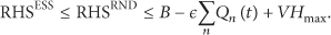
Clearly, the RHS of the randomized policy RND is given as follows:

$$\begin{array}{cc}& \text{RH}{\text{S}}^{\text{RND}}=B-{\displaystyle \sum }_n‍\mathbb{E}\left\{Q_n\left(t\right)({\widehat{\mu }}_n\left(t\right)-R_n\left(t\right))\hspace{0.17em}|\hspace{0.17em}\mathbf{Q}\left(t\right)\right\},\end{array}$$

(27)

where ${\widehat{\mu }}_n(t)$ is the transmission rate achieved by RND at time slot t. By using (16) and adding the cost function, we have

$$\begin{array}{l}B-ϵ{\displaystyle \sum }_n‍Q_n\left(t\right)+V\mathbb{E}\left({\widehat{H}}_{ϵ}\left(t\right)\hspace{0.17em}|\hspace{0.17em}\mathbf{Q}\left(t\right)\right)\\ \hspace{1em}\le B-ϵ{\displaystyle \sum }_n‍Q_n\left(t\right)+V{H}_{\max },\end{array}$$

(28)

where ${\widehat{H}}_{ϵ}(t)$ is the actual energy consumption of the randomized policy during time slot t and it depends on ϵ. By definition, $\text{RH}{\text{S}}^{\text{ESS}}\le \text{RH}{\text{S}}^{\text{RND}}$ . Then, we obtain

$$\begin{array}{cc}& \text{RH}{\text{S}}^{\text{ESS}}\le \text{RH}{\text{S}}^{\text{RND}}\le B-ϵ{\displaystyle \sum }_n‍Q_n\left(t\right)+V{H}_{\max }.\end{array}$$

(29)

Thus

$$\begin{array}{cc}& \Delta \left(t\right)+V\mathbb{E}\left(H\left(t\right)\hspace{0.17em}|\hspace{0.17em}\mathbf{Q}\left(t\right)\right)\le B-ϵ{\displaystyle \sum }_n‍Q_n\left(t\right)+V{H}_{\max }.\end{array}$$

(30)

It is straightforward to see that (30) has exactly the same form as (25). Thus, this proves the theorem.

5.3. Optimality of ESS

In this section, we show that ESS algorithm yields asymptotically optimal solution to (7). In other words, the average energy consumption proposed by the ESS algorithm can be made arbitrarily close to the global minimum solution of (7), by selecting a sufficiently large value of a real-valued constant V. The following fact from [9] establishes a bound on any scalar-valued function $g(·)$ .

Theorem 5 (Lyapunov optimization).

If (25) holds, then the time average energy satisfies the following:

$$\begin{array}{cc}& \underset{T\to \infty }{\mathrm{limsup}}\frac{\mathrm{1}}{T}{\displaystyle \sum }_{t=\mathrm{0}}^{T-\mathrm{1}}‍\mathbb{E}\left\{g\left(t\right)\right\}\le g^{\mathrm{\ast }}+\frac{B}{V}.\end{array}$$

(31)

Theorem 6.

ESS algorithm is energy optimal and satisfies (31).

Proof.

Rewriting (28) and using (29) we attain

$$\begin{array}{l}\Delta \left(t\right)+V\mathbb{E}\left(H\left(t\right)\hspace{0.17em}|\hspace{0.17em}\mathbf{Q}\left(t\right)\right)\le B-ϵ{\displaystyle \sum }_n‍Q_n\left(t\right)\\ \hspace{1em}\hspace{1em}+V\mathbb{E}\left({\widehat{H}}_{ϵ}\left(t\right)\hspace{0.17em}|\hspace{0.17em}\mathbf{Q}\left(t\right)\right).\end{array}$$

(32)

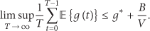
We take the expectation of both sides of (31) and obtain

$$\begin{array}{cc}& \Delta \left(t\right)+V\mathbb{E}\left(H\left(t\right)\right)\le B-ϵ\mathbb{E}\left({\displaystyle \sum }_n‍Q_n\left(t\right)\right)+V\mathbb{E}\left({\widehat{H}}_{ϵ}\left(t\right)\right).\end{array}$$

(33)

Note that inequality (33) holds for any time slot t. Hence, we sum both sides of (33) from time slot $\mathrm{0}$ to $T-\mathrm{1}$ and divide by T. As a result, we obtain

$$\begin{array}{l}\frac{\mathbb{E}\left({\sum }_n‍Q_n^{\mathrm{2}}\left(T\right)\right)}{T}-\frac{\mathbb{E}\left({\sum }_n‍Q_n^{\mathrm{2}}\left(\mathrm{0}\right)\right)}{T}+\frac{V}{T}{\displaystyle \sum }_{t=\mathrm{0}}^{T-\mathrm{1}}‍\mathbb{E}\left(H\left(t\right)\right)\\ \hspace{1em}\hspace{1em}\le B-\frac{ϵ}{T}{\displaystyle \sum }_{t=\mathrm{0}}^{T-\mathrm{1}}‍{\displaystyle \sum }_n‍\mathbb{E}\left(Q_n\left(t\right)\right)+V\mathbb{E}\left({\widehat{H}}_{ϵ}\left(t\right)\right).\end{array}$$

(34)

Recall that, in the previous section, we have shown that the second term in the RHS of (34) is bounded. By taking ${\mathrm{limsup}}_{T\to \infty }$ , we get

$$\begin{array}{cc}& \underset{T\to \infty }{\mathrm{limsup}}\frac{V}{T}{\displaystyle \sum }_{t=\mathrm{0}}^{T-\mathrm{1}}‍{\displaystyle \sum }_n‍\mathbb{E}\left(H\left(t\right)\right)\le B+V\mathbb{E}\left({\widehat{H}}_{ϵ}\left(t\right)\right).\end{array}$$

(35)

Consequently, by dividing both sides of (35) by V, we have

$$\begin{array}{cc}& \underset{T\to \infty }{\mathrm{limsup}}\frac{\mathrm{1}}{T}{\displaystyle \sum }_{t=\mathrm{0}}^{T-\mathrm{1}}‍{\displaystyle \sum }_n‍\mathbb{E}\left(H\left(t\right)\right)\le \frac{B}{V}+\mathbb{E}\left({\widehat{H}}_{ϵ}\left(t\right)\right).\end{array}$$

(36)

Note that $\mathbb{E}({\widehat{H}}_{ϵ}(t))\to h^{\mathrm{\ast }}$ as $ϵ\to \mathrm{0}$ as we have shown in the previous section. The bound in (36) is clearly minimized by taking a limit as $ϵ\to \mathrm{0}$ , which yields (31).

5.4. Distributed Implementation

Note that for the implementation of ESS algorithm a centralized authority must exist so that the switching decision can be given. In this section, we present a distributed solution to the scheduling problem (7), which does not require a centralized mechanism and thus can be easily implemented for large-scale sensor networks. Basic idea behind the distributed implementation of ESS algorithm is that each node makes its own switching decision individually. The independent decision of each node is given according to the following rule.

Rule 1.

If node n is active at time slot t, then it keeps staying in active mode as long as the following inequality holds:

$$\begin{array}{cc}& Q_n\left(t\right)>\frac{V(E_n^{\mathrm{1}}\left(t\right)-E_n^{\mathrm{0}}\left(t\right)-E_n^{\mathrm{10}}\left(t\right))}{{\mu }_n\left(t\right)},\hspace{1em}\forall n\in \mathcal{A}.\end{array}$$

(37)

Note that the switching and transmission decision for an active node with ESS algorithm are given according to (8)–(10), where only the maximizer of Rule 1 can stay in active node and transmit. However, the knowledge of the maximizer of Rule 1 requires a centralized system. On the other hand, in distributed implementation there may be more than one active node in the network at a given time slot. Thus, one can expect that ESS outperforms the distributed algorithm in terms of lifetime.

Rule 2.

If node m is at sleep mode at time slot t it remains in the sleep mode for the next time slot if the following inequality is satisfied:

$$\begin{array}{cc}& Q_m\left(t\right)<\frac{V(E_m^{\mathrm{1}}\left(t\right)+E_m^{\mathrm{01}}\left(t\right)-E_m^{\mathrm{1}}\left(t\right))}{{\mu }_m\left(t\right)},\hspace{1em}\mathrm{\hspace{0.17em}\hspace{0.17em}}\forall m\in \mathcal{S}.\end{array}$$

(38)

Otherwise, node m switches to active mode. Note that the decision of staying in sleep mode can be given independently with ESS algorithm. However, if a sleeping node needs to switch to active mode, this decision must be given by centralized ESS algorithm. However, with the distributed implementation, any sleeping node can switche to active node if Rule 2 is not satisfied. Hence, there may be more than one active node which switches from sleeping mode.

After determining the energy modes, scheduling decision is given among the active nodes. The knowledge of backlog levels in the neighboring nodes can be maintained by infrequent broadcasting. The minimum energy broadcasting methods are proposed in [28, 29], which can be applied to our model in order to find the transmissions node. Afterwards, the node which maximizes (39) is scheduled. A more formal representation of distributed implementation developed by Rule 1 and Rule 2 is given in Algorithm 1:

$$\begin{array}{cc}& \underset{n\in \mathcal{A}}{\max }\mathrm{\hspace{0.17em}\hspace{0.17em}}{Q}_n\left(t\right){\mu }_n\left(t\right)-V{E}_n^s\left(t\right)-V{E}_n^{\mathrm{1}}\left(t\right).\end{array}$$

(39)

Algorithm 1: Distributed algorithm.

(1)  Initialize: Set all nodes to the sleep mode and the remaining energy $$E_n(\mathrm{0})=E_{\text{tot}},n\in \mathcal{N},t=\mathrm{0}$$

(2)  while   $$E_n(t)$$ > 0  do

(3)           generate  packet arrivals and transmission rate

(4)           if   $$n\in \mathcal{S}$$ and $$Q_n(t)<(V(E_n^{\mathrm{1}}\left(t\right)+E_n^{\mathrm{01}}\left(t\right)-E_n^{\mathrm{0}}\left(t\right)))/{\mu }_n(t)$$   then

(5)                 compute   $$E_n(t)=E_n(t)-E_n^{\mathrm{0}}(t)$$   {compute remaining energy}

(6)                 compute   $$W_n(t)=-V{E}^{\mathrm{0}}(t)$$   {assign and compute weight}

(7)           else if   $$n\in \mathcal{S}$$ and $$Q_n(t)>(V(E_n^{\mathrm{1}}\left(t\right)+E_n^{\mathrm{01}}\left(t\right)-E_n^{\mathrm{0}}\left(t\right)))/{\mu }_n(t)$$   then

(8)                 add  node n to $$\mathcal{A}$$   {switch to active mode}

(9)                 compute   $$E_n(t)=E_n(t)-E_n^{\mathrm{01}}(t)-c(t)$$

(10)               compute   $$W_n(t)=Q_n(t){\mu }_n(t)-V(E_n^{\mathrm{01}}(t)+E_n^{\mathrm{1}}(t)+\alpha {\mu }_n(t))$$

(11)          end if

(12)          if   $$n\in \mathcal{A}$$ and $$Q_n(t)<(V(E_n^{\mathrm{1}}\left(t\right)+\alpha {\mu }_n\left(t\right)-E_n^{\mathrm{10}}\left(t\right)-E_n^{\mathrm{0}}\mathrm{\hspace{0.17em}\hspace{0.17em}}\left(t\right)))/{\mu }_n(t)$$   then

(13)                add  node n to S  {switch to sleep mode}

(14)                compute   $$E_n(t)=E_n(t)-E_n^{\mathrm{10}}(t)-E_n^{\mathrm{0}}(t)$$

(15)                compute   $$W_n(t)=-V(E_n^{\mathrm{10}}(t)+E_n^{\mathrm{0}}(t))$$

(16)          else if   $$n\in \mathcal{A}$$ and $$Q_n(t)>(V(E_n^{\mathrm{1}}\left(t\right)+\alpha {\mu }_n\left(t\right)-E_n^{\mathrm{10}}\left(t\right)-E_n^{\mathrm{0}}\left(t\right)))/{\mu }_n(t)$$   then

(17)                compute   $$E_n(t)=E_n(t)-c(t)$$

(18)                compute   $$W_n(t)=Q_n(t){\mu }_n(t)-V(c(t)+\alpha {\mu }_n(t))$$

(19)          end if

(20)          if   $$n\in \mathcal{A}$$   then

(21)                compute   $$E_n(t)=E_n(t)-E_b(t)$$   {broadcast energy $$E_b$$ (t)}

                         {broadcast its weight}

(22)                if   $$k=\arg {\max }_n{W}_n(t)$$    $$n\in \mathcal{A}$$   then

(23)                        $$E_n(t)=E_n(t)-\alpha (t){\mu }_n(t)$$

(24)                end if

(25)          end if

(26)          update   $$Q_n(t)$$

(27)           $$t=t+\mathrm{1}$$

(28) end while

6. Power Allocation with ESS

In previous sections, we assumed that all nodes transmit at full power. In practice, transmission power control is an essential part of wireless communications, and it is especially important for wireless devices with limited energy resources. In this section, our objective is to investigate performance of ESS algorithm when power control is performed.

Let $P_{\max }$ be the maximum allowed transmission power at any time slot. We define $P_n(t)$ as the transmission power of sensor node n at time slot t, where $P_n(t)\le P_{\max }$ for all n and t. The achievable transmission rate of node n is given by

$$\begin{array}{cc}& {\tilde{\mu }}_n\left(t\right)=\log \left(\mathrm{1}+\frac{M_n\left(t\right)P_n\left(t\right)}{{\sigma }^{\mathrm{2}}}\right),\end{array}$$

(40)

where $M_n(t)$ is the channel gain between node n and the sink at time slot t. ${\sigma }^{\mathrm{2}}$ is the ambient noise power. Note that when node n consumes $P_n(t)$ amount of power for a duration of $T_s$ second then it consumes $T_s\times P_n(t)$ amount of energy. Without loss of generality, we assume that $T_s$ is unit time for the rest of this section.

Recall that ESS algorithm schedules node n, for which the following function is maximized:

$$\begin{array}{cc}& W_n\left(t\right)=Q_n\left(t\right){\tilde{\mu }}_n\left(t\right)-V{E}_n^s\left(t\right)-V{\displaystyle \sum }_{z=\mathrm{0}}^{\mathrm{1}}‍E_z^n\left(t\right).\end{array}$$

(41)

Note that in (8)   $W_n(t)$ is determined by using $P_{\max }$ for all users. On the other hand, in (41) the optimal power for each user should be determined. Furthermore, the optimal power allocation should take into account the energy mode of each sensor node. Thus, we next investigate the power control problem for an arbitrary sensor node n by considering the following cases.

Case 1.

If node n is in active mode at time slot t and will remain active at the next time slot $t+\mathrm{1}$ , then it does not change its energy mode. Hence, there is no switching energy cost, and its weight is equal to $W_n(t)=Q_n(t){\mu }_n(t)-V{E}_n^{\mathrm{1}}(t)$ . Also, for this case $E_n^{\mathrm{1}}(t)=P_n(t)$ . Then, the optimal power allocation is performed as follows: $W_n(t)$ is given by

$$\begin{array}{cc}& W_n\left(t\right)=Q_n\left(t\right)\log \left(\mathrm{1}+\frac{M_n\left(t\right)P_n\left(t\right)}{{\sigma }^{\mathrm{2}}}\right)-V{P}_n\left(t\right).\end{array}$$

(42)

It can be shown that $W_n(t)$ is a concave function of $P_n(t)$ . Hence, the optimal power allocation is determined by the first order optimality conditions on $W_n(t)$ ; that is,

$$\begin{array}{cc}& \frac{d{W}_n\left(t\right)}{d{P}_n\left(t\right)}=\frac{M_n\left(t\right)Q_n\left(t\right)}{{\sigma }^{\mathrm{2}}+M_n\left(t\right)P_n\left(t\right)}-V=\mathrm{0}.\end{array}$$

(43)

After solving the equation, the optimal power allocation for node n is given by

$$\begin{array}{cc}& P_n^{\mathrm{\ast }}\left(t\right)=\min \left\{P_{\max },\max \left\{\frac{Q_n\left(t\right)}{V}-\frac{{\sigma }^{\mathrm{2}}}{M_n\left(t\right)},\mathrm{0}\right\}\right\}.\end{array}$$

(44)

Case 2.

If node n is in sleep mode at time slot t but will become active at the next time slot $t+\mathrm{1}$ , then it has to change its energy mode and there will be a switching energy cost. Thus, its weight is given by

$$\begin{array}{cc}& W_n\left(t\right)=Q_n\left(t\right){\tilde{\mu }}_n\left(t\right)-V{E}_n^s\left(t\right)-V{P}_n\left(t\right).\end{array}$$

(45)

Note that the switching energy does not depend on transmit power $P_n(t)$ . Hence, the optimal power allocation for the second case is also given by (44).

Let $W_n^{\mathrm{\ast }}(t)$ be the weight of node n with the optimal power allocation; that is,

$$\begin{array}{cc}& W_n^{\mathrm{\ast }}\left(t\right)=Q_n\left(t\right){\tilde{\mu }}_n^{\mathrm{\ast }}\left(t\right)-V{E}_n^s\left(t\right)-V{\displaystyle \sum }_{z=\mathrm{0}}^{\mathrm{1}}‍E_z^n\left(t\right),\end{array}$$

(46)

where ${\tilde{\mu }}_n^{\mathrm{\ast }}(t)=\log (\mathrm{1}+(M_n(t)P_n^{\mathrm{\ast }}(t)/{\sigma }^{\mathrm{2}}))$ .

Once the optimal power allocation is determined, the sink node acquires channel state and the queue size information of each sensor node. Then, the optimal power is determined according to (44), and the weight for each node is calculated according to (46). Then, ESS algorithm with power control determines the energy modes of operation for each sensor node and selects the transmitting node $n^{\mathrm{\ast }}$ , where

$$\begin{array}{cc}& n^{\mathrm{\ast }}=\underset{n\in \mathcal{A}}{\text{argmax}}\hspace{0.17em}{W}_n^{\mathrm{\ast }}\left(t\right).\end{array}$$

(47)

7. Numerical Results

We consider a scenario where there are 5 sensor nodes and a base station. The nodes observe their surrounding and generate random packets and transmit them to the base station in a single-hop fashion. We assume that each node has a battery with an initial energy of 10 Joules. The arrival processes are assumed to be Bernoulli processes with an average rate of 4 packets with size of 45 bytes per slot for all nodes and without loss of generality we assume that a slot is 2 millisecond (ms) long. For a particular node, there are three equally likely possible channel states, that is, Good, Medium, and Bad where the corresponding transmission rate of a node is assumed to be 20, 12, and 5 packets, respectively. The parameters used in the simulation are given by [2].

(i) Sleep Mode Energy, $E_{\mathrm{0}}$ . Nodes consume energy in sleep mode and it is equal to $\mathrm{0.015}\times \mathrm{1}{\mathrm{0}}^{-\mathrm{6}}$  J per millisecond.

(ii) Active Mode Energy, $E_{\mathrm{1}}$ . The nodes in active mode consume energy due to being in active mode, $c(t)$ , and also for the transmission of each packet, $\alpha (t)$ . Thus, $E_{\mathrm{1}}(t)=c(t)+\mu (t)\alpha (t)$ . $c(t)$ is given as $\mathrm{36}\times \mathrm{1}{\mathrm{0}}^{-\mathrm{6}}$  J per millisecond and $\alpha (t)$ is taken to be $\mathrm{30}\times \mathrm{1}{\mathrm{0}}^{-\mathrm{6}}$  J per packet transmission.

(iii) Energy due to Switching from Sleep to Active, $E_{\mathrm{01}}$ . Switching time from sleep to active is 0.7 ms and the switching energy from sleep to active is equal to $\mathrm{25.2}\times \mathrm{1}{\mathrm{0}}^{-\mathrm{6}}$  J.

(iv) Energy due to Switching from Active to Sleep, $E_{\mathrm{10}}$ . Switching time from active to sleep is 0.01 ms and the switching energy from active to sleep is equal to $\mathrm{2.85}\times \mathrm{1}{\mathrm{0}}^{-\mathrm{6}}$  J.

(v) Broadcast Energy, $E_b(t)$ . Broadcast energy is taken to be $\mathrm{8.33}\times \mathrm{1}{\mathrm{0}}^{-\mathrm{8}}$  J per bit.

If a sensor node is in sleep mode at the beginning of a time slot and wants to switch to active mode, then the switching takes 0.7 ms. Thus, the sensor can stay in active mode for a duration of 1.3 ms since total slot duration is 2 ms second. Additionally, it consumes a packet transmission energy if it is selected by ESS algorithm. As a result, it consumes an amount of energy which is equal to $\mathrm{1.3}\hspace{0.17em}\text{ms}\times c(t)+\alpha \mu (t)$ . When the node keeps its energy mode, then there will be no switching energy and the energy consumption will be equal to only the sleep energy, $E_{\mathrm{0}}(t)$ . On the other hand, if an active sensor is selected to be the active node the next slot, then it can use entire slot for its own transmission since there will be no switching time and the energy consumption will be $\mathrm{2}\hspace{0.17em}\text{ms}\times c(t)+\alpha \mu (t)$ . If it switches the sleep mode, the energy spent by the node will be equal to $\mathrm{1.99}\hspace{0.17em}\text{ms}\times E_{\mathrm{0}}(t)+E_{\mathrm{10}}$ .

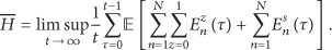
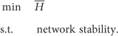
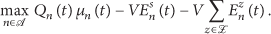
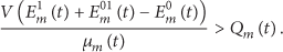
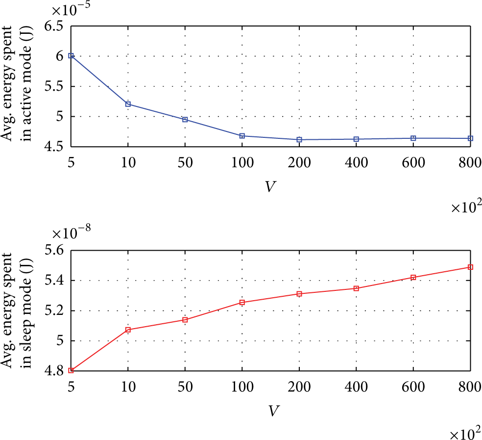
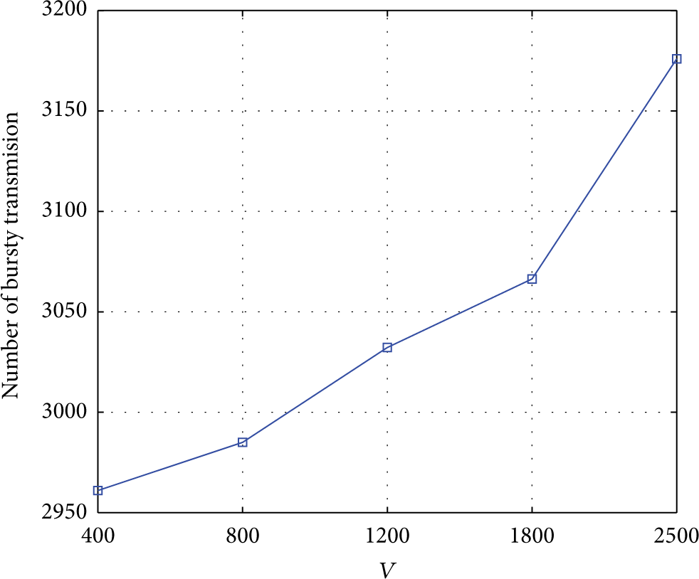
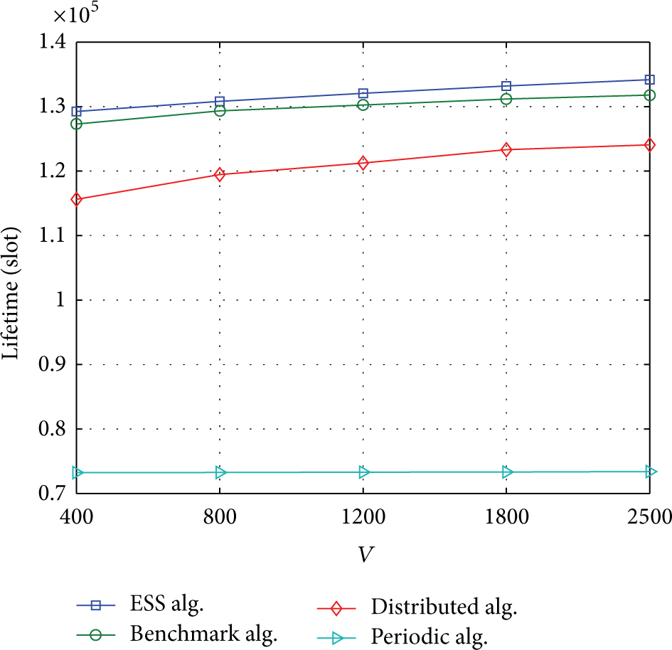
First, we investigate the average energy consumption in sleep and active modes for $V=500$ , 1000, 5000, 10000, 20000, 40000, 60000, and $\mathrm{80000}$ . Figure 1 depicts the average energy spent in active and sleep modes. As V grows, the nodes run out their batteries by staying in sleep mode most of the time. This prolongs their lifetime since they consume the minimum energy in sleep mode and this result agrees with Theorem 6. Due to the fact that the nodes can not transmit in sleep mode, it yields an increase in queue sizes of the nodes and consequently average delay in the network increases. Next, we conduct a simulation experiment to observe the bursty departure property of ESS algorithm explained in Lemma 1. As stated in Lemma 1, the nodes transmit their packets consecutively in order to reduce the switching energy. Figure 2 depicts the average number of bursty active staying which is the number of two or more consecutive time slots where the node is selected to be the active node and transmits. Higher values of V push the nodes to spend the minimum energy and in order not to consume switching energy the nodes are selected as the active node in a bursty fashion. Furthermore, we compare the ESS algorithm with a “benchmark algorithm” and the S-MAC type algorithm proposed in [30], namely, “periodic algorithm,” in terms of the average queue backlogs for different values of $V=\mathrm{400}$ , 800, 1200, 1800, 2500. Contrary to ESS, the benchmark algorithm ignores the switching energy and makes the switching and scheduling decisions without considering switching energy cost. Therefore, the nodes change their modes more frequently. In S-MAC type periodic algorithm, the nodes stay in sleep mode during the first 1 ms and, during the last 1 ms, they stay in active mode. Furthermore, the node which maximizes $Q_n(t){\mu }_n(t)-V\alpha {\mu }_n(t)$ is selected as the transmitting node during the active period. As it is seen in Figure 3, the benchmark algorithm outperforms ESS in terms of the queue backlogs, since it stays in the active mode at most of the time. On the other hand, since ESS promotes the nodes to stay in sleep mode considering the switching cost, it prolongs the network lifetime. The periodic algorithm has the worst performance since it has fixed duty cycle property which can not ensure the efficient time to reduce the queue backlogs as much as ESS algorithm. Figure 4 depicts the comparison of the lifetime performance induced by ESS, the benchmark, and the distributed and the periodic algorithms. The distributed algorithm allows more than one node to be active at any time slot and the benchmark algorithm does not care about the switching energy cost. In addition, the periodic algorithm forces the nodes to be active for 1 ms at every slot and, due to the fixed duty cycle, V does not affect the lifetime of periodic algorithm. Thus, with these algorithms, the nodes stay in active mode unnecessarily. As a result, batteries of the node run out quickly. Therefore, EES shows better performance result in terms of lifetime. Finally, Figure 5 depicts the average duty cycle of the network per node. As V increases, the proportion of time the nodes stay in active mode decreases to prevent the energy consumption. Thus, the average duty cycle period decreases as well. It is easy to see that the duty cycle per node can be approximately at most 13%. As stated in [2], the switching energy needs to be computed if the node duty cycle is low. Thus, the effect of switching energy becomes significant.

Figure 1

Average energy consumptions in active and sleep modes.

Figure 2

Bursty transmission.

Figure 3

The average queue backlogs for different values of V.

Figure 4

The network lifetime for different values of V.

Figure 5

Duty cycle.

8. Conclusion

In this paper, we investigate the energy efficiency and optimal control problems in a low duty cycle wireless sensor network. Using Lyapunov optimization technique, an energy-aware switching and scheduling (ESS) algorithm is proposed. The switching energy is generally not considered in energy management problems. However, analysis indicates that ESS algorithm outperforms the benchmark algorithm which ignores the switching energy cost in terms of the lifetime. Furthermore, we show that we can stabilize the network by applying ESS algorithm and push its performance to the optimal solution by tuning V parameter. In addition, we present a distributed algorithm that can be implemented easily. In terms of future work, we investigate scheduling problem for multihop sensor networks.