Sage Journals: Discover world-class research

Abstract

Owning to the proliferation of cost-effective sensors, there has been an increased growth in a number of applications of wireless sensor networks (WSNs). In addition, the skyline operator as well as its variants such as the dynamic skyline and reverse skyline operator has attracted increasing attention since those are useful for multicriteria decision making applications. Since the energy efficiency is utmost important issue to prolong the network lifetime, in this paper, we proposed efficient algorithms to process a reverse skyline query over a sliding window in WSN environments. We first devise our algorithm for the data stream environments and extend it to WSN environments. To compute the reverse skyline, we partition the data space into several orthants with respect to a query point. And, in each orthant, we compute the reverse skyline independently using two buffers. In our experiment study, we demonstrate that our algorithm is much better than other algorithms.

1. Introduction

Since being introduced in the database community, the skyline operator [1] and its variants such as dynamic skyline [2] and reverse skyline [3] operators have attracted increasing attention in multicriteria decision making applications such as product recommendations [4, 5], querying wireless sensor networks [6], and graph analysis [7].

Given a d-dimensional point set P, a point $p_{i} \in P$ dominates another point $p_{j} \in P$ if $p_{i}$ is smaller than $p_{2}$ in at least one dimension and not greater than $p_{2}$ in all other dimensions. The skyline on P comprises all points that are not dominated by any other points. Papadias et al. [2] proposed the dynamic skyline which is a set of points in P not to be dynamically dominated by any other point with respect to (wrt) coordinate-wise distances to a given query point q. Another interesting skyline variant is the reverse skyline operator which returns a set of every point in P, denoted as $R S L (q, P)$ , whose dynamic skyline contains a query point q [3].

In general, a wireless sensor network (WSN) is considered as a cost effective platform to monitor environments. A WSN consists of spatially distributed devices with various sensors and a powered base station which serves as an access point for users to pose ad hoc queries. The research for diverse types of queries over WSNs, for example data gathering [8], aggregation queries [9, 10], join queries [11, 12], and skyline queries [6, 13, 14], has been conducted to satisfy the diverse application demands. Among the diverse types of queries, a reverse skyline query is very useful for environmental monitoring applications. For example, in an application of monitoring the forest environment, a lot of sensors are deployed in a forest to collect sensor readings such as temperature and humidity. Assume a query point q represents the thresholds of a possible fire disaster on different attributes.

A naive method to detect a forest fire with a query point q is that only the sensor nodes with sensor readings exceeding thresholds report their sensor reading. For instance, let each point in Figure 1(a) represent the sensor reading of each sensor node. Since many sensor readings, represented by dotted circles in Figure 1(a), exceed the thresholds, many sensor nodes consume much energy to transmit a lot of sensor readings. Because each sensor node is battery-powered and located in hazardous or hard-to-reach place, it is impossible or very difficult to change the batteries of sensor nodes. Thus, in WSN environments, the energy efficiency is the utmost important issue to prolong the network lifetime.

Figure 1

An example for a forest fire.

In contrast to the naive method, the reverse skyline operator considers the dominance relationship for attributes with respect to a query point q which indicates a potential fire disaster as shown in Figure 1(b). The reverse skyline points are represented by dotted circles in Figure 1(b). A point $p_{i}$ is a reverse skyline point when q is a dynamic skyline point wrt $p_{i}$ . In other words, q is not dynamically dominated by other points wrt $p_{i}$ . Informally, it means that q and $p_{i}$ are close to each other at least in one dimension (i.e., q and $p_{i}$ are similar to each other compared to other points at least in one dimension). Thus, the reverse skyline can represent the sensor nodes having sensor readings highly following the fire pattern for at least one attribute compared with others. Therefore, this can save much time and quickly locate the most dangerous places.

In this paper, we investigate the problem of energy-efficient in-network reverse skyline computation in WSN environments. In particular, WSN can be considered as a source of data streams. The data stream can be broken into possibly overlapping partitions by specifying a window and computation can be carried out in each partition. While efficient processing techniques for window queries have been proposed in the area of data streams, most of the previous work on data stream processing assumes that query processing is conducted at a centralized server. On contrary, in-network processing is commonly used in sensor network where each sensor calculates a partial result. Therefore, in our work, we devise an energy efficient algorithm to compute the reverse skyline considering sliding window queries which return repeatedly reverse skyline points during a given time interval. In this paper, we consider the sensor readings that arrived in a sliding window with size w. Specifically, a sensor reading generated at time $t_{s}$ is alive during $[t_{s}, t_{e}) = [t_{s}, t_{s} + w)$ .

Our Contributions. Our work has the following combination of contributions to perform the reverse skyline operator over a sliding window. (i)

To make an efficient algorithm of the reverse skyline, we analyze the properties of the reverse skyline theoretically. At first, we divide the d-dimensional data space into $2^{d}$ orthants wrt a query point q. Then, we prove that every reverse skyline point wrt q is also a dynamic skyline point wrt q on each orthant and any dynamic skyline point dominated by a midpoint of another point in each orthant is not a reverse skyline point.

(ii)

Each sensor node can be regarded as a source of stream data since each sensor node measures its environment repeatedly. Thus, we first proposed an effective algorithm which computes reverse skyline for a sliding window over a data stream. The devised algorithm is running on each sensor node to generate partial result. To compute the reverse skyline progressively, our algorithm maintains two buffers $o . B u f f_{d s k y}$ and $o . B u f f_{r e s t}$ on each orthant o which keep the dynamic skyline points and the dynamic skyline candidates, respectively.

(iii)

We devise in-network reverse skyline processing technique in WSN environments. Each node in a WSN only transmits small number of points to its parent node when the points become newly dynamic skyline points or the states of them are changed. Accordingly, the energy consumption of each node decreases.

To evaluate our proposed algorithms, we implemented our algorithms. In our experiments, we use the synthetic data set and the real-world data set to show the effectiveness of our algorithms in data stream environments and WSN environments. In data stream environments, we measure the processing time of each algorithm and, in WSN environments, we measure the total energy consumption of every node. Our comprehensive empirical evaluation demonstrates that our algorithm delivers the best performance in all situations.

The rest of the paper is organized as follows. Section 2 introduces the various skyline operators and wireless sensor networks. Section 3 contains related work. We present the basic features of the reverse skyline and propose our basic algorithm to process the reverse skyline in Section 4. In Section 5, we present the energy efficient in-network processing technique to compute reverse skyline over sliding window in WSN environments. Section 6 presents the empirical evaluation results and Section 7 summarizes the paper.

2. Preliminaries

2.1. Various Skyline Operators

Formally, given a d-dimensional data set $P = {p_{1}, \dots, p_{| P |}}$ , a point $p_{i} \in P$ is represented as $p_{i} = 〈 p_{i} \cdot x_{1}, p_{i} \cdot x_{2}, \dots, p_{i} \cdot x_{d} 〉$ , where $p_{i} \cdot x_{k}$ is the value of $p_{i}$ 's kth coordinate. A point $p_{i}$ dominates another point $p_{j}$ , denoted as $p_{i} ≺ p_{j}$ , if the two conditions hold: (1) $\forall k \in {1, \dots, d}$ , $p_{i} \cdot x_{k} \leq p_{j} \cdot x_{k}$ and (2) $\exists k \in {1, \dots, d}$ , $p_{i} \cdot x_{k} < p_{j} \cdot x_{k}$ . Based on the dominance relationship, the skyline of P is defined as follows.

Definition 1 (skyline).

Given a d-dimensional data set $P = {p_{1}, \dots, p_{| P |}}$ , the skyline of P, represented by $SL (P)$ , is largest subset of P where every point in $SL (P)$ is not dominated by any other point in P. In other words, $SL (P) = {p_{i} \in P | ∄ p_{j} (\neq p_{i}) \in P s.t. p_{j} ≺ p_{i}}$ .

Given a d-dimensional query point q, the dominance relationship extended the dynamic dominance relationship. We say that a point $p_{i}$ dynamically dominates $p_{j}$ with respect to (wrt) q, denoted as $p_{i} ≺_{q} p_{j}$ , if $\forall k \in {1, \dots, d}$ , $| p_{i} \cdot x_{k} - q_{k} |$ ≤ $| p_{j} \cdot x_{k} - q \cdot x_{k} |$ , and $\exists k \in {1, \dots, d}$ , $| p_{i} \cdot x_{k} - q_{k} |$ < $| p_{j} \cdot x_{k} - q \cdot x_{k} |$ .

Definition 2 (dynamic skyline).

Given a d-dimensional data set P and a query point q, the dynamic skyline of P with respect to q is represented by $D S L (q, P)$ such that $D S L (q, P) = {p_{i} \in P |$ ∄ $p_{j} (\neq p_{i}) \in P$ s.t. $p_{j} ≺_{q} p_{i}}$ .

Based on the dynamic skyline, the notion of the reverse skyline was proposed in [3]. The reverse skyline is defined as the follows.

Definition 3 (reverse skyline).

Given a d-dimensional data set P and a query point q, the reverse skyline, represented by $R S L (q, P)$ , is the set of every point $p_{i}$ in P satisfying $q \in D S L (p_{i}, P \cup {q} - {p_{i}})$ .

Example 4.

Consider the data set $P = {p_{1}, \dots, p_{7}}$ in Figure 2(a). Given a query point q represented by ★, a point $p_{4}$ is a dynamic skyline point wrt q since $p_{4}$ is not dynamically dominated by the other points. However, since a point $p_{5}$ is dynamically dominated by $p_{7}$ , $p_{5}$ is not a dynamic skyline. The dynamic skyline of P wrt q is $D S L (q, P) = {p_{3}, p_{4}, p_{7}}$ in Figure 2(a). Figure 2(b) shows the dynamic skyline wrt $p_{7}$ . Since q is not a dynamic skyline point wrt $p_{7}$ , $p_{7}$ is a reverse skyline point (i.e., $p_{7} \notin R S L (q, P)$ ). As shown in Figure 1(b), $R S L (q, P) = {p_{3}}$ .

Figure 2

An example of the dynamic skyline.

2.2. Wireless Sensor Networks

We consider a sensor network consisting of n stationary sensor nodes ${s_{1}, s_{2}, \dots, s_{n}}$ deployed in a field of interest and a powered base station serving as an access point for users to pose ad hoc queries. As a basic primitive to collect sensing data in WSNs, we use an ad hoc spanning tree, such as TinyDB [15] and SNEE [16] as the basic routing structure from each sensor node to the base station. Figure 3 illustrates an example of simple sensor network consisting of eight sensor nodes.

Figure 3

A simple sensor network.

To form a routing tree, the base station first sends a request message which contains a hop-counter indicating the hop distance from the base station. When each node $s_{c}$ receives a request message from another node $s_{p}$ , if $s_{c}$ does not have a parent node yet, node $s_{p}$ becomes the parent node of $s_{c}$ , and, then, $s_{c}$ forwards the request message with the hop-counter increased by 1 to the other nodes. If $s_{c}$ already has a parent, $s_{c}$ simply ignores the request message. When $s_{c}$ receives several request messages from the other nodes, $s_{c}$ picks the one which has the smallest hop-counter as the parent. To break ties, the heuristics such as signal strength and arrival time can be applied. A sensor reading consists of several attributes each of which is associated with a sensor module. A sensor node may be equipped with several sensor modules. Sensor nodes generate their readings periodically and synchronously. To synchronize the sampling time, every sensor node executes a global time synchronization protocol [17].

3. Related Work

To reduce the energy consumption of WSNs, research on diverse types of queries such as aggregation, data gathering, join, and skyline has been conducted. One of the well-known approaches to reduce the energy consumption of WSNs is in-network processing. In the in-network processing techniques, the partial results are progressively merged at intermediate nodes on their way to the base station according to the tree routing.

3.1. Aggregation

The pioneering TAG work by Madden et al. in [9] studied in-network aggregation for reducing communication overhead using summary data (e.g., SUM) and/or exemplary data (e.g., MIN and MAX). In TAG, as climbing up a routing tree from leaf nodes to the base station, partial aggregation values are computed. Approximate aggregation techniques have been also proposed to reduce the energy consumption. The work of Considine et al. [18] was based on the FM sketch. Shrivastava et al. [19] developed the q-digest structure to support approximate processing for quantile queries such as MEDIAN. In [20], an effective aggregation technique for the situation that sensor nodes can detect an object duplicately was presented. To identify the duplicates eagerly, a variant of bloom filers was utilized in [20]. Refer to [21] for the summary of in-network aggregation.

3.2. Data Gathering

For the situations that require the sensor readings rather than an aggregate value, some approximate sensor data gathering techniques have been proposed since most applications of sensor networks do not require highly accurate data. Some correlations appear among sensor readings. Such correlations can be captured by standard techniques like the linear regression and statistical distribution functions. Basically, each sensor estimates its readings independently with its own model. And the mirror model for each sensor is in the base station. Thus, if a sensor node does not transmit a sensor reading, the base station can obtain an approximate reading using the mirror model.

BBQ [22] uses the multivariate Gaussian to model the sensor readings instead of data interval. Chu et al. [23] extends BBQ by partitioning the sensor field to cliques in order to utilize the spatial correlation. Since the optimal partitioning is NP-hard, Ken uses the greedy heuristics. Jain et al. suggested dual Kalman filter [24] which is based on the Kalman filter. In addition, Min and Chung proposed EDGES [25] based on a variant of the Kalman filter, that is, multimodel Kalman filter. In [8], by utilizing the spatial correlation such that the change patterns of sensor readings of the neighbor sensors are the same or similar, an effective data gathering technique was presented.

3.3. Join

In some applications, a user wants to identify the relationship between sensor readings in different regions. This regional correlation can be expressed as a join query of sensor readings in two regions. Thus, recently, research on in-network join processing has been proposed to reduce the communication overhead. Some works [26, 27] study how to find an optimal join location using the cost models. In these works, the optimal join location is near to the weighted centroid of three points: the center points of two regions and the base station.

Some in-network join techniques utilize a semijoin operator which filters out one of the relations based on the join attribute values of the other relation. However, due to a large number of join attribute values, a lot of energy is consumed. To alleviate this overhead, some work utilizes the synopsis of join attribute values. In [28], a histogram based semijoin approach is proposed. Stern et al. propose the method called SENS-Join [29], which is similar to that of [28], in order to avoid shipping tuples through the network that do not participate in the joins. As the compact representation, they use pointless quadtree representation.

3.4. Skyline

After Börzsönyi et al. [1] proposed the skyline operator, various techniques [30, 31] have been presented to improve the performance of skyline queries. The sort-filter skyline (SFS) algorithm [30] improves BNL using presorted data set according to the scores computed by a monotone function. By exploiting R^*-tree, Kossmann et al. [31] presented an improved algorithm, called NN, based on the nearest neighbor search. The dynamic skyline was introduced by Papadias et al. [2]. Later on, the reverse skyline was proposed by Dellis and Seeger [3].

Since the skyline operator as well as its variants is useful to detect interesting events, there are some studies for in-network skyline processing in WSN environments. In [13], a filtering technique was proposed to reduce the energy consumption of WSNs in which some filter points are broadcasted to every sensor node and the data points dominated by the filter points are not transmitted since they cannot be in the skyline. Recently, a multiple filter-based algorithm called SKYFILTER was proposed to processing skyline over the sliding window in [14]. However, to compute filter points, every sensor node wastes its energy. The most related literature to our work is [6]. To obtain the reverse skyline points in WSNs, the 2-Skyband query that retrieves every point which is dominated by at most one point wrt q is used. However, this technique calculates the reverse skyline with the currently generated points only. In other words, the reverse skyline processing over a sliding window is not supported. In contrast to previous work, we investigate effective reverse skyline processing techniques over a sliding window in data stream environments as well as WSN environments.

4. Reverse Skyline Processing over Sliding Windows

Before the presentation of the overall behavior of our proposed in-network reverse skyline processing, we first present the properties of the reverse skyline in Section 4.1. Since each sensor node in WSNs generates its readings continuously, each sensor node can be considered as a source of stream data. Thus, in Section 4.2, we present our basic algorithm in the context of stream data. Our in-network processing technique based on the basic algorithm will be presented in Section 5.

4.1. Properties of Reverse Skyline

In this section, we present the properties of the reverse skyline. Park et al. [32] showed that, when the d-dimensional space is divided into $2^{d}$ orthants with respect to a query point q as shown in Figure 4, the reverse skyline can be computed with each subset $P_{o} \subset P$ independently, where $P_{o}$ denotes the set of points located in each orthant o.

Figure 4

Subsets $P_{(o = 1 \dots 4)}$ in P.

Lemma 5.

Given a data set P, a query point q, and an orthant o, if and only if a point $p_{i} \in P_{o} \subseteq P$ is not in $R S L (q, P)$ , then there exists another $p_{j}$ in $P_{o}$ which dynamically dominates q with respect to $p_{i}$ (i.e., $p_{j} ≺_{p_{i}} q$ ).

Proof.

(:⇐) For $p_{i}$ , $p_{j}$ ∈ $P_{o}$ , if $p_{j} ≺_{p_{i}} q$ , q is not a dynamic skyline with respect to $p_{i}$ (i.e., $q \notin D S L (p_{i}, P \cup {p} - {q_{i}}$ )). By Definitions 2 and 3, $p_{i}$ is not in $R S L (q, P)$ .

(⇒:) If a point $p_{i} \in P_{o}$ is not in $R S L (q, P)$ , there exists $p_{j}$ such that $p_{j} ≺_{p_{i}} q$ by Definition 3. Then we have $| q \cdot x_{k} - p_{i} \cdot x_{k} |$ ≥ $| p_{j} \cdot x_{k} - p_{i} \cdot x_{k} |$ ∀ $k \in {1, \dots, d}$ . Squaring both sides, we get $0 \geq (p_{j} \cdot x_{k} - p_{i} \cdot x_{k})^{2} - (q \cdot x_{k} - p_{i} \cdot x_{k})^{2}$ . Rearranging terms, we have $0 \geq (p_{j} \cdot x_{k} + q \cdot x_{k} - 2 p_{i} \cdot x_{k})$ · $(p_{j} \cdot x_{k} - q \cdot x_{k}) = - 2 \cdot (p_{i} \cdot x_{k} - q \cdot x_{k}) (p_{j} \cdot x_{k} - q \cdot x_{k}) + (p_{j} \cdot x_{k} - q \cdot x_{k})^{2}$ . Since $2 \cdot (p_{i} \cdot x_{k} - q \cdot x_{k})$ · $(p_{j} \cdot x_{k} - q \cdot x_{k})$ ≥ $(p_{j} \cdot x_{k} - q \cdot x_{k})^{2} \geq 0$ ∀ $k \in {1, \dots, d}$ , $(p_{i} \cdot x_{k} - q \cdot x_{k})$ and $(p_{j} \cdot x_{k} - q \cdot x_{k})$ have the same sign. Thus, $p_{j}$ is also in $P_{o}$ .

By Lemma 5, we have $R S L (q, P) = \cup_{\forall P_{o}} R S L (q, P_{o})$ . Now, for brevity, we explain our algorithm on a single orthant o and the corresponding data set $P_{o} \subseteq P$ .

The following lemma addresses that every reverse skyline point wrt q is also a dynamic skyline point wrt q but not vice versa.

Lemma 6.

Given an orthant o and a query point q, $R S L (q, P_{o})$ ⊆ $D S L (q, P_{o})$ .

Proof.

For the purpose of contradiction, we assume $p_{i} (\in P_{o}) \notin D S L (q, P_{o})$ . Thus, there exists $p_{j} \in P_{o}$ such that $p_{j} ≺_{q} p_{i}$ , and, hence, $| p_{j} \cdot x_{k} - q \cdot x_{k} |$ ≤ $| p_{i} \cdot x_{k} - q \cdot x_{k} |$ ∀ $k \in {1, \dots, d}$ (and $\exists k \in {1, \dots}$ , $| p_{j} \cdot x_{k} - q \cdot x_{k} |$ < $| p_{i} \cdot x_{k} - q \cdot x_{k} |$ ). It means that $p_{i} \cdot x_{k}$ is located farther than $p_{j} \cdot x_{k}$ from $q \cdot x_{k}$ in the orthant o. It implies that $p_{j} \cdot x_{k}$ is closer to $p_{i} \cdot x_{k}$ than $q \cdot x_{k}$ is. Obviously, $| p_{j} \cdot x_{k} - p_{i} \cdot x_{k} |$ ≤ $| q \cdot x_{k} - p_{i} \cdot x_{k} |$ $\forall k$ (and $\exists k$ , $| p_{j} \cdot x_{k} - p_{i} \cdot x_{k} |$ < $| q \cdot x_{k} - p_{i} \cdot x_{k} |$ ). Then, we have $p_{j} ≺_{p_{i}} q$ . Thus, $p_{i} \notin R S L (q, P_{o})$ . Therefore, $R S L (q, P_{o})$ ⊆ $D S L (q, P_{o})$ .

From Lemma 6, in order to compute the reverse skyline of each $P_{o}$ , a nonreverse skyline point in $D S L (q, P_{o})$ should be eliminated. For this purpose, we utilize the idea of midpoints introduced in [3, 6, 32]. The midpoint $m_{i}$ of a point $p_{i}$ with respect to a query point q is defined as $m_{i} = 〈 (p_{i} \cdot x_{1} + q \cdot x_{1}) / 2, (p_{i} \cdot x_{2} + q \cdot x_{2}) / 2, \dots, (p_{i} \cdot x_{d} + q \cdot x_{d}) / 2 〉$ .

Lemma 7.

Given an orthant o and a query point q, $p_{i} \in D S L (q, P_{o})$ is not a reverse skyline if there exists another point $p_{j} \in P_{o}$ whose midpoint dynamically dominates $p_{i}$ with respect to q (i.e., $m_{j} ≺_{q} p_{i}$ ).

Proof (by contradiction).

Assume that $p_{i} \in R S L (q, P_{o}) \subset D S L (q, P_{o})$ . Since $p_{i} \in R S L (q, P_{o})$ , there does not exist $p_{j} \in P_{o}$ s.t.; $p_{j} ≺_{p_{i}} q$ . Then, in the proof of Lemma 5, we infer that there does not exist $p_{j} \in P_{o}$ satisfying $2 \cdot (p_{i} \cdot x_{k} - q \cdot x_{k}) \cdot (p_{j} \cdot x_{k} - q \cdot x_{k}) \geq (p_{j} \cdot x_{k} - q \cdot x_{k})^{2} \forall k \in {1, \dots, d}$ .

However, when $m_{j} ≺_{q} p_{i}$ , we have $| (p_{j} \cdot x_{k} + q \cdot x_{k}) / 2 - q \cdot x_{k} |$ = $| p_{j} \cdot x_{k} - q \cdot x_{k} | / 2$ ≤ $| p_{i} \cdot x_{k} - q \cdot x_{k} | \forall k \in {1, \dots, d}$ . By multiplying $2 \cdot (p_{j} \cdot x_{k} - q \cdot x_{k})$ to both sides, we get $(p_{j} \cdot x_{k} - q \cdot x_{k})^{2} \leq 2 \cdot (p_{j} \cdot x_{k} - q \cdot x_{k}) (p_{i} \cdot x_{k} - q \cdot x_{k})$ . Therefore, by contradiction, $p_{i} \notin R S L (q, P_{o})$ if $m_{j} ≺_{q} p_{i}$ .

Example 8.

Consider a data set P in Figure 4. By Lemma 5, we can compute the reverse skyline on each orthant o independently.

Given a data set $P_{4} = {p_{1}, p_{2}, p_{3}} \subset P$ , as shown in Figure 5, since each point in $P_{4}$ is not dynamically dominating each other wrt q, every point is a dynamic skyline point (i.e., $D S L (q, P_{4}) = P_{4}$ ). However, a midpoint $m_{2}$ of $p_{2}$ dynamically dominates $p_{1}$ wrt q. Thus, by Lemma 7, $p_{1}$ is not a reverse skyline point (i.e., $p_{1} \notin R S L (q, P_{4})$ ). Similarly, $p_{2}$ does not belong to $R S L (q, P)$ , either. In this example, $p_{3}$ , denoted as a bold circle, is a reverse skyline point since $p_{3}$ is not dynamically dominated by any midpoint wrt q except its midpoint $m_{3}$ .

Figure 5

Midpoints in an orthant.

4.2. Computing $R S L (q, P_{o})$ over Sliding Windows

In this section, we present our algorithm, called RSPW, to compute reverse skyline over sliding windows in WSNs by utilizing the properties of reverse skyline presented in Section 4.1. Basically, RSPW is working on each sensor node to generate partial reverse skyline. In Section 5, we will present how to integrate the partial reverse skyline generated by each sensor node.

To compute the skyline over a sliding window, Tao and Papadias [33] proposed an effective method. Similarly, we need to keep the dynamic skyline based on Lemma 6 to obtain the reverse skyline. Thus, we adapt the sliding window skyline processing technique (denoted as SWSP) proposed in [33] to our reverse skyline processing over sliding windows.

Lemma 9 (see [33]).

Let $p_{i}$ be a point in $D B$ . If $p_{i}$ is dominated by a newly generated point $p_{j}$ , then $p_{i}$ can be safely discarded from $D B$ ; that is, $p_{i}$ will not be part of the skyline in the future.

Since SWSP is for the skyline processing, SWSP considers a single data space. In addition, SWSP handles the database $DB$ (i.e, the set of points which are alive) based on Lemma 9. Meanwhile, by Lemma 5, we can compute the reverse skyline on each orthant independently. For each orthant o, two buffers $o . B u f f_{d s k y}$ and $o . B u f f_{r e s t}$ are maintained in our work. In addition, although SWSP maintains $DB$ efficiently based on Lemma 9, Lemma 9 does not hold in our work since we need to prune out the nonreverse skyline points from $D S L (q, P_{o})$ by Lemma 7.

For instance, as shown in Figure 6(a), $p_{1}$ and $p_{2}$ were generated where a point $p_{i}$ is generated at time i. Let a window size w be $3$ . As shown in Figure 6(a), when time t is 2, $p_{2}$ dynamically dominates $p_{1}$ wrt q. Thus, $p_{1}$ is not a dynamic skyline point nor a reverse skyline point either. Meanwhile, $p_{2}$ is a dynamic skyline point but is not a reverse skyline point since the midpoint $m_{1}$ of $p_{1}$ dynamically dominates $p_{2}$ . To indicate whether a dynamic skyline point is not a reverse skyline, we assign a mark to the point which is not a reverse skyline point. Note that, even though we use a mark, we cannot discard $p_{1}$ simply in this example.

Figure 6

An example for a sliding window ( $w = 3$ ).

As shown in Figure 6(b), $p_{1}$ expires when time $t = 4$ since w = $3$ . If other points are not generated within the time interval [13, 30], $p_{2}$ should become a reverse skyline point at $t = 4$ since no midpoint dominates $p_{2}$ . In this case, if we discard $p_{1}$ at t = $2$ , we do not have a time information for $p_{2}$ being a reverse skyline point. In other words, a mark itself is not sufficient to preserve the dominance relationship with respect to time. To keep such information, each mark has an expiry time. In Figure 6(a), a mark with an expiry time $t_{\exp}$ is represented by “ $*, t_{\exp}$ .”

In our work, $o . B u f f_{d s k y}$ keeps the dynamic skyline in the orthant o at the current time. Every nonreverse skyline point among the dynamic skyline points has a mark with its expire time. $o . B u f f_{r e s t}$ maintains the dynamic skyline candidates which will be a part of the dynamic skyline in the future. To maintain $o . B u f f_{d s k y}$ and $o . B u f f_{r e s t}$ , we devise the following proposition and lemma.

Proposition 10.

Given a query point q and an orthant o, every point $p_{i}$ in $o . B u f f_{d s k y} \cup o . B u f f_{r e s t}$ dynamically dominated by the midpoint of a newly generated point $p_{j}$ could not be a reverse skyline point for $p_{j}$ 's lifespan.

Proof.

It trivially holds by Lemma 7.

By Proposition 10, when a point $p_{j}$ appears in an orthant o at time j, every point $p_{i} \in (o . B u f f_{d s k y} \cup o . B u f f_{r e s t})$ dynamically dominated by $m_{j}$ of $p_{j}$ is assigned a mark with expiry time (i.e., $t_{\exp}$ ) as $p_{j} \cdot t_{e}$ .

Lemma 11.

Given a query point q and an orthant o, every point $p_{k}$ in $o . B u f f_{d s k y}$ and $o . B u f f_{r e s t}$ dynamically dominated by a newly generated point $p_{j}$ (i.e., $p_{j} ≺_{q} p_{k}$ ) can be discarded. In addition, if there is a point $p_{i}$ such that $p_{i}$ has the largest expiry time among the points in $o . B u f f_{d s k y} \cup o . B u f f_{r e s t}$ whose midpoints dynamically dominate $p_{j}$ , then $p_{j}$ cannot be a reverse skyline point within $p_{i}$ 's lifespan.

Proof.

By Definition 2, given a new point $p_{j}$ , every $p_{k} \in (o . B u f f_{d s k y}$ ∪ $o . B u f f_{r e s t})$ such that $p_{j} ≺_{q} p_{k}$ cannot be a dynamic skyline point. In addition, since $p_{j}$ is newly generated, every $p_{k}$ will expire before $p_{j}$ . Thus, every $p_{k}$ cannot be a reverse skyline point within its lifespan due to $p_{j}$ . In addition, by definition of midpoints, if $p_{j} ≺_{q} p_{k}$ , then $m_{j} ≺_{q} m_{k}$ . Thus, since every point dynamically dominated by $m_{k}$ is also dynamically dominated by $m_{j}$ , we can discard $p_{k}$ . Meanwhile, by Lemma 7, since the point $p_{i}$ is the point whose expire time is largest among the points whose midpoints dynamically dominate $p_{j}$ , $p_{j}$ cannot be a reverse skyline during $p_{i}$ 's lifespan.

By Lemma 11, $p_{j} \in P_{o}$ has a mark with expiry time as $ma x_{p_{i} \in P_{o}^{j}} (p_{i} \cdot t_{e})$ where $P_{i}^{j}$ = ${p_{i} \in (o . B u f f_{d s k y}$ ∪ $o . B u f f_{r e s t}) | m_{i} ≺_{q} p_{j}}$ . In addition, we can remove every point $p_{i}$ in $o . B u f f_{d s k y}$ and $o . B u f f_{r e s t}$ if $p_{i}$ is dynamically dominated by the incoming point $p_{j}$ .

The pseudocode of our proposed algorithm, denoted by RSPW, is presented in Pseudocode 1. The algorithm RSPW computes the reverse skyline over a sliding window. RSPW consists of two parts. The first one is for processing a newly created point $p_{j}$ at the current time j (lines 1–12 in Pseudocode 1). The other one is for managing expired points and expired marks at the current time j (lines 14–20).

Pseudocode 1: The pseudocode of RSPW.

Procedure $R S P W (P_{o})$

// $P_{o}$ is an input stream and this is invoked at each time j

//the midpoint of a point $p_{i}$ is denoted as $m_{i}$

begin

(1) Let $p_{j}$ be a newly generated point at the current time j and located on an orthant o;

(2) mark_time = 0

(3) is_dsky = $t r u e$

(4) for each point $p_{i}$ ∈ ( $o . B u f f_{d s k y}$ ∪ $o . B u f f_{r e s t}$ ) do {

(5) if $p_{i} ≺_{q} p_{j}$ then is_dsky = $f a l s e$

(6) if $m_{i} ≺_{q} p_{j}$ and mark_time < $p_{i} \cdot t_{e}$ then mark_time = $p_{i} \cdot t_{e}$ //Lemma 11

(7) if $p_{j} ≺_{q} p_{i}$ then remove $p_{i}$ //Lemma 11

(8) else if $m_{j} ≺_{q} p_{i}$ then mark $p_{i}$ where $t_{\exp} = p_{j} \cdot t_{e}$ //Proposition 10

(9) }

(10) if mark_time ≠ 0 then mark $p_{j}$ where $t_{\exp}$ = mark_time //Lemma 11

( $11$ ) if is_dsky = $t r u e$ then insert $p_{j}$ into $o . B u f f_{d s k y}$

( $12$ ) else insert $p_{j}$ into $o . B u f f_{r e s t}$

( $13$ )

(14) for each point $p_{i}$ ∈ $o . B u f f_{d s k y}$ do {

( $15$ ) if $p_{i} \cdot t_{e}$ = j then {// $p_{i}$ expires at this time

( $16$ ) move every $p_{k} \in o . B u f f_{r e s t}$ which is exclusively dominated by $p_{i}$ to $o . B u f f_{d s k y}$

( $17$ ) remove $p_{i}$ from $o . B u f f_{d s k y}$

( $18$ ) }

( $19$ ) else if $p_{i}$ has a mark and $t_{\exp} = j$ then unmark $p_{i}$

(20) }

(21) return $o . B u f f_{d s k y}$

end

Recall that we maintain two buffers for each orthant o: $o . B u f f_{d s k y}$ and $o . B u f f_{r e s t}$ . Given a sliding window sized w, $o . B u f f_{d s k y}$ maintains the dynamic skyline points in the orthant o. The nonreverse skyline points in $o . B u f f_{d s k y}$ are annotated with marks. The buffer $o . B u f f_{r e s t}$ keeps the dynamic skyline candidates which can be a reverse skyline in the future.

When a new point $p_{j}$ is generated at the current time j in an orthant o (line 1), RSPW investigates whether $p_{j}$ is a dynamic skyline point or not by comparing with every point $p_{i}$ in $o . B u f f_{d s k y}$ and $o . B u f f_{r e s t}$ . If $p_{j}$ is dynamically dominated by $p_{i}$ , since $p_{j}$ cannot be a dynamic skyline, the flag is_dsky sets to $f a l s e$ (line 5). If there is a point $p_{i}$ such that the midpoint $m_{i}$ of $p_{i}$ dynamically dominates $p_{j}$ , $p_{j}$ should have a mark with an expiry time. Thus, based on Lemma 11, RSPW maintains the largest expiry time for $p_{j}$ 's mark in mark_time (line 6). In addition, RSPW removes $p_{i}$ if $p_{i}$ is dynamically dominated by Lemma 11. When $p_{i}$ is not dynamically dominated by $p_{j}$ , $p_{i}$ can become a dynamic skyline point. But if $p_{i}$ is dynamically dominated by the midpoint $m_{j}$ of $p_{j}$ , since $p_{i}$ will not be a reverse skyline point, we assign a mark with an expiry time as $p_{j} \cdot t_{e}$ to $p_{i}$ due to Proposition 10 (line 8). After iterating all points in $o . B u f f_{d s k y}$ and $o . B u f f_{r e s t}$ , RSPW assigns a mark with mark_time to $p_{j}$ if it is required (line 10). And $p_{j}$ is inserted into $o . B u f f_{d s k y}$ or $o . B u f f_{r e s t}$ with respect to the flag is_dsky (lines 11-12).

When a point $p_{i}$ is expired at the current time j (i.e., $p_{i} \cdot t_{e} = j$ ) (line 15), $p_{i}$ should be eliminated. By elimination of $p_{i}$ , every point $p_{k}$ in $o . B u f f_{r e s t}$ which is dynamically dominated by $p_{i}$ exclusively becomes dynamic skyline point at time j. Thus, the algorithm RSPW moves such $p_{k}$ in $o . B u f f_{r e s t}$ to $o . B u f f_{d s k y}$ and removes $p_{i}$ (lines 15–18). In addition, RSPW unmarks every point $p_{i}$ in $o . B u f f_{d s k y}$ whose mark's expiry time is j (line 19).

Finally, the set of dynamic skyline point (i.e., $o . B u f f_{d s k y}$ ) is returned (line 21). Recall that every nonreverse skyline point has a mark. Thus, we can easily identify reverse skyline points from the dynamic skyline points in $o . B u f f_{d s k y}$ .

The following example illustrates the behavior of our proposed algorithm RSPW within a single orthant o.

Example 12.

Let the size of window w be $2$ and each point $p_{t}$ be generated at time t. Figure 7(a) shows the states of the points generated when t is $1$ to $4$ . When $t = 1$ , since there is $p_{1}$ only in an orthant o, $p_{1}$ is a dynamic skyline point (and a reverse skyline point), and, hence, $p_{1}$ is in $o . B u f f_{d s k y}$ . When $t = 2$ , since $p_{2}$ is dynamically dominated by $p_{1}$ , $p_{2}$ is in $o . B u f f_{r e s t}$ . In addition, since the midpoint $m_{2}$ of $p_{2}$ dynamically dominates $p_{1}$ , $p_{1}$ is annotated with a mark $*, 4$ . Since $p_{2}$ is also dynamically dominated by $m_{1}$ , $p_{2}$ has a mark $*, 3$ . When $t = 3$ , since $p_{3}$ is not dynamically dominated by any other point as well as the other midpoints, $p_{3}$ becomes a reverse skyline point and is in $o . B u f f_{d s k y}$ . In addition, since $p_{1}$ 's expiry time is 3, $p_{1}$ is removed, and, then, $p_{2}$ becomes a dynamic skyline point. Thus, $p_{2}$ moves to $o . B u f f_{d s k y}$ . Furthermore, the expiry time of $p_{2}$ 's mark is 3, and $p_{2}$ becomes a reverse skyline point.

As shown in Figure 7(b), since $p_{2} \cdot t_{e} = 4$ , $p_{2}$ is expired when $t = 4$ . Since $p_{4}$ dominates $p_{3} \in o . B u f f_{d s k y}$ , $p_{4}$ becomes a dynamic skyline point and $p_{3}$ is discarded. Since $m_{3}$ does not dynamically dominate $p_{4}$ , $p_{4}$ has no mark (i.e., $p_{4}$ is a reverse skyline point at $t = 4$ ). In addition, when $t = 5$ , $p_{5}$ is newly generated. Since $p_{5}$ and $p_{4}$ do not dynamically dominate each other, $p_{5}$ and $p_{4}$ are dynamic skyline points as well as $p_{4}$ is not removed. However, since their midpoints $m_{4}$ and $m_{5}$ dynamically dominate $p_{5}$ and $p_{4}$ , respectively, $p_{4}$ and $p_{5}$ have marks.

Figure 7

The behavior of RSPW.

Up to now, we present our algorithm to compute the reverse skyline over a sliding window in data stream environments. In the next section, we will describe how to calculate the reverse skyline in WSN environments.

5. Energy Efficient RSPW for WSNs

As mentioned above, the energy efficiency is the utmost important in WSN environments. A brute-force algorithm, denoted as ${R S P W}_{b f}$ , to compute reverse skyline over a sliding window in WSNs is that every sensor node transmits its sensor readings to the base station along the routing path and the base station computes dynamic skyline using the algorithm RSPW presented in Section 4.2 and extracts reverse skyline points having no mark. However, since each sensor node blindly sends its readings to the base station, each sensor node consumes much energy.

Based on the following lemma, we can apply RSPW to each sensor node in WSNs.

Lemma 13.

Given an orthant o, a query point q, and two sensor nodes $s_{1}$ and $s_{2}$ , let $P_{o}^{1}$ and $P_{o}^{2}$ be the set of points located in o and generated by $s_{1}$ and $s_{2}$ , respectively. Then, $p_{i}$ is in RSPW( $P_{o}^{1} \cup P_{o}^{2}$ ) iff $p_{i}$ is in RSPW( $P_{o}^{1} \cup R S P W (P_{o}^{2})$ ), where RSPW( $P_{o}^{k}$ ) returns $o . B u f f_{d s k y}$ of $P_{o}^{k}$ . In addition, $p_{i}$ in RSPW( $P_{o}^{1} \cup P_{o}^{2}$ ) has a mark iff $p_{i}$ in RSPW( $P_{o}^{1} \cup R S P W (P_{o}^{2})$ ) has a mark.

Proof.

Assume that $p_{i}$ ∉RSPW $(P_{o}^{1} \cup P_{o}^{2})$ (i.e, $p_{i}$ is not a dynamic skyline point in ( $P_{o}^{1}$ ∪ $P_{o}^{2}$ )). Then there is another point $p^{'}$ in ( $P_{o}^{1}$ ∪ $P_{o}^{2}$ ) such that $p^{'} ≺_{q} p_{i}$ . Let the result of RSPW( $P_{o}^{2}$ ) be $o^{2} . B u f f_{d s k y}$ for brevity. If $p^{'}$ ∈ $P_{o}^{1}$ , $p_{i}$ is not in RSPW( $P_{o}^{1} \cup R S P W$ ( $P_{o}^{2}$ )) trivially. Otherwise, if $p^{'}$ ∈ $P_{o}^{2}$ and $o^{2} . B u f f_{d s k y}$ , $p_{i}$ cannot be in RSPW( $P_{o}^{1} \cup R S P W$ ( $P_{o}^{2}$ )) either. If $p^{'}$ ∈ $P_{o}^{2}$ but not in $o^{2} . B u f f_{d s k y}$ , since $p^{'}$ is not a dynamic skyline point in $P_{o}^{2}$ , there exists $p^{''}$ in $o^{2} . B u f f_{d s k y}$ such that $p^{''} ≺_{q} p^{'} (≺_{q} p_{i})$ . Consequently, $p_{i} \in$ RSPW( $P_{o}^{1} \cup P_{o}^{2}$ ) iff $p_{i} \in$ RSPW( $P_{o}^{1} \cup R S P W$ ( $P_{o}^{2}$ )).

Now, we assume that $p_{i}$ in RSPW( $P_{o}^{1} \cup P_{o}^{2}$ ) has a mark and $p_{i}$ in RSPW( $P_{o}^{1} \cup R S P W$ ( $P_{o}^{2}$ )) does not have mark. Since $p_{i}$ has a mark, there is a point $p_{j}$ in $P_{o}^{1} \cup P_{o}^{2}$ , where the midpoint $m_{j}$ of $p_{j}$ dynamically dominates $p_{i}$ . If $p_{j}$ is in $P_{o}^{1}$ , $p_{i}$ in RSPW( $P_{o}^{1} \cup R S P W$ ( $P_{o}^{2}$ )) has also a mark trivially. Otherwise (i.e., $p_{j} \in P_{o}^{2}$ ), if $p_{j}$ is in $o^{2} . B u f f_{d s k y}$ , $p_{i} \in$ RSPW( $P_{o}^{1} \cup R S P W$ ( $P_{o}^{2}$ )) also have a mark. Thus, in order not to have a mark, $p_{j}$ should not be in $o^{2} . B u f f_{d s k y}$ . It implies that $\exists p_{j}^{'} \in o^{2} . B u f f_{d s k y}$ s.t. $p_{j}^{'} ≺_{q} p_{j}$ . By definition of midpoints, $m_{j}^{'} ≺_{q} m_{j}$ , and, hence, we have $m_{j}^{'} ≺_{q} p_{i}$ . Therefore, $p_{i} \in$ RSPW( $P_{o}^{1} \cup R S P W$ ( $P_{o}^{2}$ )) must have a mark. Since the proof for the case that $p_{i}$ in RSPW( $P_{o}^{1} \cup P_{o}^{2}$ ) does not have a mark and $p_{i}$ in RSPW( $P_{o}^{1} \cup R S P W$ ( $P_{o}^{2}$ )) has mark is similar to the above, we omit it for brevity.

By Lemma 13, a simple extension of RSPW to WSN environments is that, at each time, a sensor node performs RSPW with its sensor reading and the dynamic skyline points coming from its child nodes to maintain its $o . B u f f_{d s k y}$ and $o . B u f f_{r e s t}$ as well as transmiting $o . B u f f_{d s k y}$ to its parent node. And, then, the parent node performs RSPW and so on. In this way, the base station obtains the complete $o . B u f f_{d s k y}$ for each orthant o. We denote the simple extension of RSPW to WSNs as ${I n - N e t R S P W}_{s i m}$ .

Since each sensor node transmits $o . B u f f_{d s k y}$ only in ${I n - N e t R S P W}_{s i m}$ , each sensor node can reduce its energy consumption. However, in ${I n - N e t R S P W}_{s i m}$ , a dynamic skyline point in a sensor node's $o . B u f f_{d s k y}$ can be transmitted redundantly (at most w times) within a window sized w. It incurs energy waste. Thus, we present an enhanced algorithm, referred to as ${I n - N e t R S P W}_{e n h}$ , which is also based on Lemma 13. The pseudocode of ${I n - N e t R S P W}_{e n h}$ is presented in Pseudocode 2.

Pseudocode 2: The pseudocode of ${I n - N e t R S P W}_{e n h}$ .

Procedure ${I n - N e t R S P W}_{e n h} ()$

begin

//This is invoked at each time j

// $P_{o}^{i}$ is the input stream of this sensor node $s_{i}$

//Let $o . B u f f^{s e n t}$ be the set of points sent previously

(1) for each orthant o do {

(2) $o . B u f f^{t e m p}$ = $\emptyset$

(3) for each child node $s_{c}$ do {

(4) $o . B u f f^{t e m p}$ = $o . B u f f^{t e m p}$ ∪ receiveFromChild( $s_{c}$ );

(5) }

(6) $P_{o}^{i}$ = $P_{o}^{i} \cup B u f f^{t e m p}$

(7) $o . R e s u l t$ = $R S P W (P_{o}^{i})$

(8) remove every point $p_{k} \in o . B u f f^{s e n t}$ where $p_{k} \cdot t_{e} = j$

(9) unmark every point $p_{k} \in o . B u f f^{s e n t}$ where $t_{\exp} = j$

(10) for each point $p_{k} \in o . R e s u l t$ do {

(11) if $p_{k} \in o . B u f f^{s e n t}$ then {

(12) if $p_{k} \in o . R e s u l t$ has not a mark and $p_{k} \in o . B u f f^{s e n t}$ has not a mark then

(13) remove $p_{k}$ from $o . R e s u l t$

(14) else if $p_{k} \in o . R e s u l t$ has a mark and $p_{k} \in o . B u f f^{s e n t}$ has a mark then

(15) remove $p_{k}$ from $o . R e s u l t$

(16) else {

(17) remove $p_{k}$ from $o . B u f f^{s e n t}$

(18) $o . B u f f^{s e n t}$ = $o . B u f f^{s e n t} \cup {p_{k}}$

(19) }

(20) } else $o . B u f f^{s e n t}$ = $o . B u f f^{s e n t} \cup {p_{k}}$

(21) }

(22) sendToParent( $o . R e s u l t$ )

(23) }

end

The intuition of ${I n - N e t R S P W}_{e n h}$ is that a sensor reading becoming a dynamic skyline point newly and/or a dynamic skyline point which has a mark recently is transmitted only rather than transmitting all dynamic skyline points at each time in order to reduce the energy consumption of each sensor node. To do this, each sensor node $s_{i}$ has $o . B u f f^{s e n t}$ which consists of the dynamic skyline points (i.e., sensor readings) sent to its parent previously.

At first, each sensor node $s_{i}$ collects sensor readings coming from its child nodes into $o . B u f f^{t e m p}$ (lines 2–5). Then, $s_{i}$ conducts RSPW with its sensor readings and sensor readings coming from its child nodes and the result of RSPW is kept in $o . R e s u l t$ (lines 6-7). Before eliminating the point sent previously from $o . R e s u l t$ , we remove every expired point from $o . B u f f^{s e n t}$ and unmark the point whose mark's expire time (i.e., $t_{\exp}$ ) is this time (lines 8-9). Then, every point $p_{k}$ in $o . R e s u l t$ is evaluated on whether $p_{k}$ was sent previously (lines 10–17). If $p_{k}$ was sent (i.e., $p_{k}$ is in $o . B u f f^{s e n t}$ ) and the status of $p_{k}$ is not changed, we do not need to send $p_{k}$ (lines 11–15). Otherwise, the old $p_{k}$ in $o . B u f f^{s e n t}$ is removed and the new $p_{k}$ is inserted into $o . B u f f^{s e n t}$ to maintain $o . B u f f^{s e n t}$ properly (lines 16–19). If $p_{k}$ was not sent, $p_{k}$ is inserted in $o . B u f f^{s e n t}$ (line 20). Finally, a sensor node $s_{i}$ sends $o . R e s u l t$ to its parent (line 22).

Since ${I n - N e t R S P W}_{e n h}$ transmits new dynamic skyline points and the dynamic skyline points whose states are changed, the energy consumption of ${I n - N e t R S P W}_{e n h}$ is much smaller than those of ${I n - N e t R S P W}_{s i m}$ and the brute-force algorithm ${R S P W}_{b f}$ . We will show the energy efficiency of ${I n - N e t R S P W}_{e n h}$ by conducting experiments with a real-life data set.

6. Performance Study

We empirically evaluated the performances of our proposed algorithms in two environments: data stream environments and WSN environments. In data stream environments, we measured the processing time of our proposed algorithm RSPW and other algorithms with the synthetic data sets. On contrary, in WSN environments, we present the energy consumption of our algorithms ${I n - N e t R S P W}_{s i m}$ and ${I n - N e t R S P W}_{e n h}$ with a real data set to show the effectiveness of our algorithms. All experiments were conducted on Intel i5 platform with MS-Windows 7 and 4GB MBytes of main memory.

6.1. Experiments in Data Stream Environments

6.1.1. Experimental Environments

We performed this experiment to compare the execution time of RSPW with Naive and 2-Skyband [6]. In Naive algorithm, each point in a window is compared with the other points in a window to check whether it is a reverse skyline point or not. In addition, since 2-Skyband [6] did not consider the sliding window, we extended 2-Skyband to the sliding window context which computed 2-skyband with recent w points at each time.

In order to evaluate the performance of each algorithm over diverse environments, we used three synthetic data sets which are generated by independent, correlated, and anticorrelated as shown in Figure 8. These three data sets are commonly used to evaluate the performance of the skyline operator as well as its variants [1, 32].

Figure 8

Example of data sets (2-dimension).

Table 1 shows the parameters used in this experiment. Each synthetic data set consists of 100,000 points. We ran all algorithms 10 times with different query points generated randomly and report the average execution times. We varied the number of data points' dimension from 2 to 10 as well as the windows size of a query from 2 to 10.

Table 1

Parameters.

Parameter	Default	Range
Number of points	100,000	100,000
Number of queries	10	10
Number of dimensions (d)	6	2~10
Window size (w)	6	2~10

6.1.2. Experimental Results

Figure 9 shows the execution time of each algorithm according to the data sets with default values of the parameters. As shown in Figure 9, our proposed algorithm RSPW is the best performer. In average over all data sets, RSPW achieves up 9.23 times faster than Naive and 4.73 times faster than 2-Skyband. In correlated and anticorrelated data sets, since the data distributions are skewed, a large number of points are dominated by a few points in each orthant and hence the number of reverse skyline points is small. Meanwhile, since the points are uniformly distributed in independent data set, the number of reverse skyline points is larger than those of the other data sets. Thus, the processing time for the independent data set is worse than those for the other data sets.

Figure 9

Execution time over each data set.

With varying d from 2 to 10, we plot the execution time of each algorithm in Figure 10. As shown in Figure 10, as the number of dimensions d increases, the running time of each algorithm also increases since the overhead evaluating dominance relationship becomes increase with increasing d. However, the performance gap between RSPW and the other algorithms increases over all data sets as d increases since RSPW calculates the reverse skyline efficiently using two buffers.

Figure 10

Varying d.

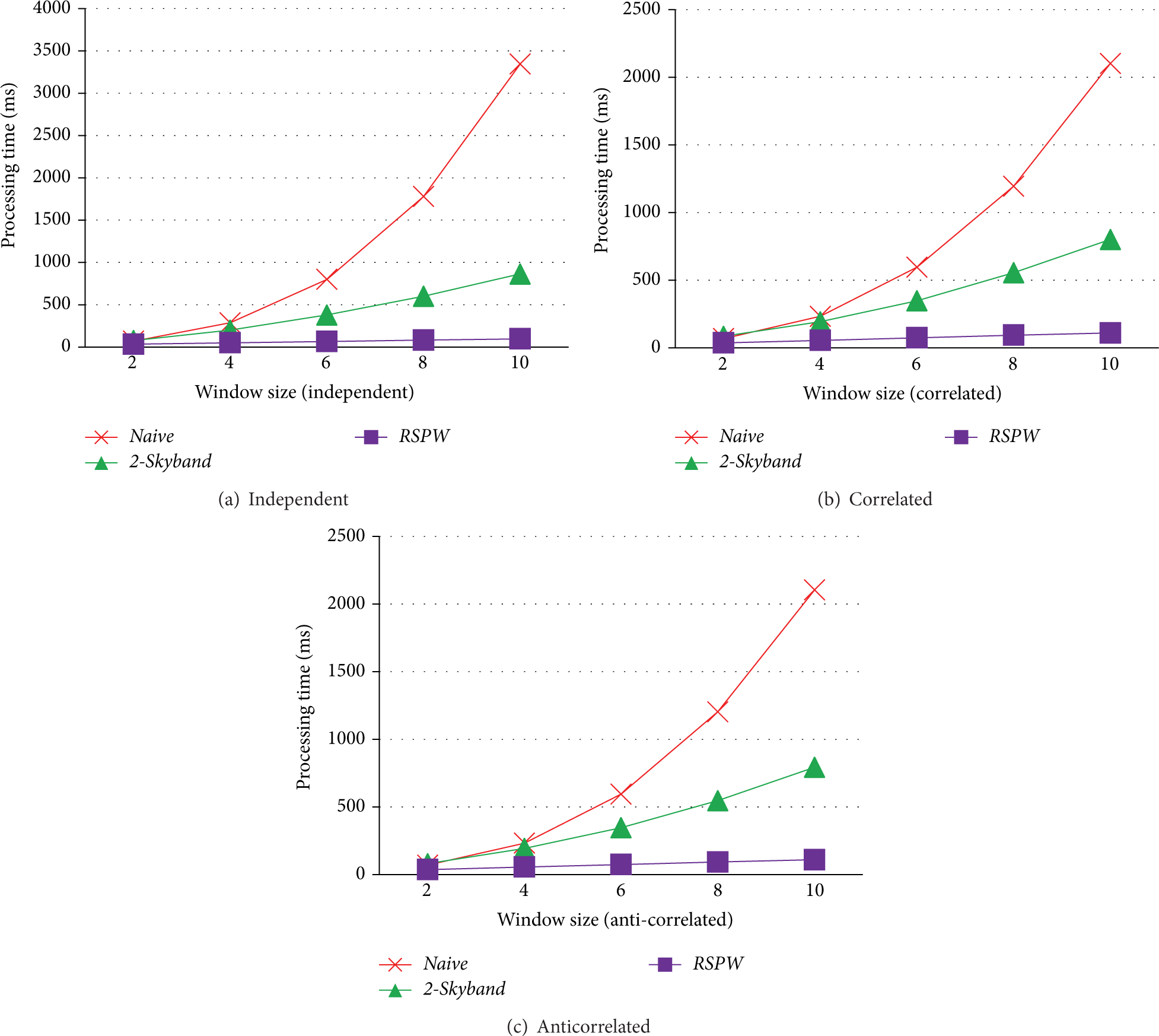
We varied w from 2 to 10 and present the running times of the algorithms in Figure 11. As illustrated in Figure 11, when the window size w is small (i.e., $w = 2$ ), all algorithms show the similar performances. However, as w increases, the execution times of Naive and 2-Skyband increase dramatically. In contrast, the execution time of RSPW increases slowly. This result indicates that RSPW computes reverse skyline efficiently over a sliding window.

Figure 11

Varying w.

6.2. Experiments in WSN Environments

6.2.1. Experimental Environments

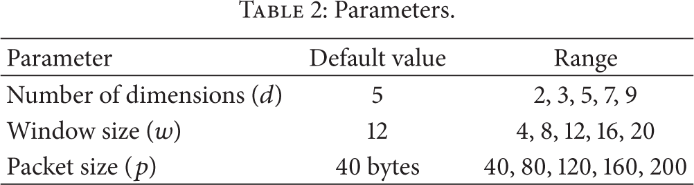
We show show the effectiveness of our proposed algorithms for WSNs with a real-life data set. As a real-life data set, we used the data LUCE provided by Audiovisual Communications Laboratory [34]. A sensor network is composed of 89 nodes deployed on the EPFL campus as shown in Figure 12 and they measured key environmental quantities at high spatial and temporal resolution over a year. The data set consists of 9 attributes such as surface temperature, solar radiation, relative humidity, rain meter, and wind speed. The size of the sensing field is 277 × 430 meter² and the base station is located at the center of the sensing field. To make a routing tree, we set the communication distance to 55 meter. The average depth (i.e., average number of child nodes) and the maximum width of the routing tree are 4.94 and 13, respectively. Since, in the real-life data set, the values of sensor readings are fixed, it is hard to make diverse configuration. Instead, to simulate diverse environments, we used some parameters. The parameters used for our experimental study are summarized in Table 2.

Table 2

Parameters.

Parameter	Default value	Range
Number of dimensions (d)	5	2, 3, 5, 7, 9
Window size (w)	12	4, 8, 12, 16, 20
Packet size (p)	40 bytes	40, 80, 120, 160, 200

Figure 12

Placement of sensor nodes.

For this experiment, we implemented ${R S P W}_{b f}$ , ${I n - N e t R S P W}_{s i m}$ , and ${I n - N e t R S P W}_{e n h}$ presented in Section 5. To compute the energy consumption of each algorithm, we used the free space channel model [35]. Under this model, to transmit a l-bits message and a distance c, a sensor expends $E_{T} (l, c) = E_{T - elec} (l) + E_{T - amp} (l, c) = l * E_{elec} + ξ_{amp} * l * c^{2}$ . And, to receive this message, a sensor expends $E_{R} (l) = E_{R - elec} (l) = l * E_{elec}$ . In this experiment, we set 50 nJ/bit to the electronic circuit constant ( $E_{elec}$ ) and 100 pJ/bit/meter² to the transmit amplifier constant ( $ξ_{amp}$ ). Like the experiments in data stream environments, we executed all algorithms 10 times with different query points generated randomly and report the average energy consumption of a network for 100,000 time units.

6.2.2. Experimental Results

We plotted the total energy consumption of the sensor network varying diverse parameter values in Figure 13. Figure 13(a) shows the consumed energy of each algorithm varying d. As the number of dimensions d increases, the energy consumption of each algorithm increases since the size of data to be transmitted increases. However, since our algorithms ${I n - N e t R S P W}_{s i m}$ and ${I n - N e t R S P W}_{e n h}$ transmit the dynamic skyline points only to the base station, the energy consumptions of ${I n - N e t R S P W}_{s i m}$ and ${I n - N e t R S P W}_{e n h}$ are less than that of ${R S P W}_{b f}$ in which every sensor node sends its readings to the base station blindly.

Figure 13

The total energy consumption with the real-life data set.

With varying the window size w from 2 to 10, we plot the energy consumption of each algorithm in Figure 13(b). Since, in ${R S P W}_{b f}$ , each sensor sends its readings, the energy consumption of ${R S P W}_{b f}$ is not affected by the window size w. Interestingly, when w becomes large, the energy consumptions of our algorithms decrease. As w increases, the lifespan of each point also increases. Thus, when a point $p_{i}$ becomes a dynamic skyline point, it will stay in $o . B u f f_{d s k y}$ for a long time and the number of points dynamically dominated by $p_{i}$ increases as w increases. Therefore, the data volume to be transmitted decreases in our algorithms since ${I n - N e t R S P W}_{s i m}$ and ${I n - N e t R S P W}_{e n h}$ transmit the dynamic skyline points in $o . B u f f_{d s k y}$ . Furthermore, ${I n - N e t R S P W}_{e n h}$ is better than ${I n - N e t R S P W}_{s i m}$ since ${I n - N e t R S P W}_{e n h}$ avoids redundant transmissions.

Figure 13(c) presents the consumed energy of each algorithm varying the packet size p. As the packet size p increases, the number of transmissions decreases since many points can be in a packet. Thus, the energy consumption of each algorithm decreases with increasing p. However, our enhanced algorithm ${I n - N e t R S P W}_{e n h}$ shows the best performance.

7. Conclusion

In this paper, we present an algorithm RSPW to compute the reverse skyline over a sliding window. To calculate the reverse skyline, we divide d-dimensional data space into $2^{d}$ orthants. Basically, RSPW computes the reverse skyline in each orthant independently. If a dynamic skyline point in an orthant is dominated by the midpoint of another point, it is annotated with a mark since it cannot be a reverse skyline. To denote the valid time of a mark within a window, each mark has an expire time. We also extend RSPW to WSN environments. Since our enhanced algorithm ${I n - N e t R S P W}_{e n h}$ transmits new dynamic skyline points and the dynamic skyline points which has a mark recently, the energy consumption of each sensor node is reduced. We implemented our algorithms and conducted an extensive evaluation with synthetic and real-life data sets. In our experiments, we demonstrated that the performance of our proposed algorithm is significantly better than other algorithms in data stream environments as well as WSN environments.

Footnotes

Conflict of Interests

The author declares that there is no conflict of interests regarding the publication of this paper.

Acknowledgment

This work was supported by Defense Acquisition Program Administration and Agency for Defense Development under Contract UD140022PD, Republic of Korea.

References

Börzsönyi

Kossmann

Stocker

The skyline operator

Proceedings of the 17th IEEE International Conference on Data Engineering (ICDE '01)

April 2001

421 430

2-s2.0-0035008034

Papadias

Tao

Seeger

An optimal and progressive algorithm for skyline queries

Proceedings of the ACM SIGMOD International Conference on Management of Data (SIGMOD '03)

June 2003

San Diego, Calif, USA

467 478

Dellis

Seeger

Efficient computation of reverse skyline queries

Proceedings of the 33rd International Conference on Very Large Data Bases (VLDB '07)

2007

291 302

Lee

won Hwang

Nie

Wen

J.-R.

Navigation system for product search

Proceedings of the 26th International Conference on Data Engineering (ICDE '10)

March 2010

Long Beach, Calif, USA

Levandoski

J. J.

Mokbel

M. F.

Khalefa

M. E.

Preference query evaluation over expensive attributes

Proceedings of the 19th International Conference on Information and Knowledge Management and Co-Located Workshops (CIKM '10)

October 2010

Ontario, Canada

319 328

10.1145/1871437.1871481

2-s2.0-78651315372

Wang

Xin

Chen

Liu

Energy-efficient reverse skyline query processing over wireless sensor networks

IEEE Transactions on Knowledge and Data Engineering 2012 24 7 1259 1275

10.1109/tkde.2011.64

2-s2.0-84861724464

Zou

Chen

Özsu

M. T.

Zhao

Dynamic skyline queries in large graphs

Proceedings of the 15th International Conference on Database Systems for Advanced Applications (DASFAA '10)

April 2010

Tsukuba, Japan

62 78

Min

J.-K.

CMOS: efficient clustered data monitoring in sensor networks

The Scientific World Journal 2013 2013 11

704957

10.1155/2013/704957

2-s2.0-84896335923

Madden

Franklin

M. J.

Hellerstein

J. M.

Hong

Tag: a tiny aggregation service for ad-hoc sensor networks

Proceedings of the 5th Symposium on Operating Systems Design and Implementation (OSDI '02)

December 2002

Boston, Mass, USA

10.

Silberstein

Munagala

Yang

Energy-efficient monitoring of extreme values in sensor networks

Proceedings of the ACM SIGMOD International Conference on Management of Data (SIGMOD '06)

June 2006

169 180

10.1145/1142473.1142493

2-s2.0-34250670478

11.

Abadi

D. J.

Madden

Lindner

REED: robust, efficient filtering and event detection in sensor networks

Proceedings of the 31st International Conference on Very Large Data Bases (VLDB '05)

September 2005

769 780

2-s2.0-33745621357

12.

Min

J.-K.

Kim

Shim

TWINS: efficient time-windowed in-network joins for sensor networks

Information Sciences 2014 263 87 109

10.1016/j.ins.2013.09.026

MR3158687

2-s2.0-84894900406

13.

Chen

Liang

Progressive skyline query processing in wireless sensor networks

Proceedings of the 5th International Conference on Mobile Ad-Hoc and Sensor Networks (MSN '09)

December 2009

17 24

10.1109/msn.2009.43

2-s2.0-77949929464

14.

Roh

Y. J.

Song

Jeon

J. H.

Woo

K. G.

Kim

M. H.

Energy-efficient two-dimensional skyline query processing in wireless sensor networks

Proceedings of the IEEE 10th Consumer Communications and Networking Conference (CCNC '13)

January 2013

294 301

10.1109/ccnc.2013.6488461

2-s2.0-84875972132

15.

Madden

S. R.

Franklin

M. J.

Hellerstein

J. M.

Hong

TinyDB: an acquisitional query processing system for sensor networks

ACM Transactions on Database Systems 2005 30 1 122 173

10.1145/1061318.1061322

2-s2.0-23944487783

16.

Galpin

Brenninkmeijer

C. Y. A.

Gray

A. J. G.

Jabeen

Fernandes

A. A. A.

Paton

N. W.

Snee: a query processor for wireless sensor networks

Distributed and Parallel Databases 2011 29 1-2 31 85

10.1007/s10619-010-7074-3

2-s2.0-78650900246

17.

Sundararaman

Buy

Kshemkalyani

A. D.

Clock synchronization for wireless sensor networks: a survey

Ad Hoc Networks 2005 3 3 281 323

10.1016/j.adhoc.2005.01.002

2-s2.0-13944269967

18.

Considine

Kollios

Byers

J. W.

Approximate aggregation techniques for sensor databases

Proceedings of the 20th International Conference on Data Engineering (ICDE '04)

March-April 2004

449 460

10.1109/icde.2004.1320018

2-s2.0-2442576849

19.

Shrivastava

Buragohain

Agrawal

Suri

Medians and beyond: new aggregation techniques for sensor networks

Proceedings of the 2nd International Conference on Embedded Networked Sensor Systems (SenSys '04)

November 2004

ACM

239 249

2-s2.0-27644511275

10.1145/1031495.1031524

20.

Min

J.-K.

R. T.

Shim

Aggregate query processing in the presence of duplicates in wireless sensor networks

Information Sciences 2015 297 1 20

10.1016/j.ins.2014.11.021

MR3291887

21.

Fasolo

Rossi

Widmer

Zorzi

In-network aggregation techniques for wireless sensor networks: a survey

IEEE Wireless Communications 2007 14 2 70 87

10.1109/mwc.2007.358967

2-s2.0-34248662954

22.

Deshpande

Guestrin

Madden

Hellerstein

J. M.

Hong

Model-driven data acquisition in sensor networks

Proceedings of the 30th International Conference on Very Large Data Bases (VLDB '04)

August 2004

Trondheim, Norway

588 599

23.

Chu

Deshpande

Hellerstein

J. M.

Hong

Approximate data collection in sensor networks using probabilistic models

Proceedings of the 22nd International Conference on Data Engineering (ICDE '06)

April 2006

10.1109/icde.2006.21

2-s2.0-33749644725

24.

Jain

Chang

E. Y.

Wang

Y.-F.

Adaptive stream resource management using Kalman Filters

Proceedings of the ACM SIGMOD International Conference on Management of Data (SIGMOD '04)

June 2004

11 22

2-s2.0-3142770653

25.

Min

J.-K.

Chung

C.-W.

EDGES: efficient data gathering in sensor networks using temporal and spatial correlations

Journal of Systems and Software 2010 25 5 933 944

26.

Coman

Nascimento

M. A.

Sander

On join location in sensor networks

Proceedings of the 8th International Conference on Mobile Data Management (MDM '07)

May 2007

190 197

10.1109/mdm.2007.35

2-s2.0-48649096273

27.

Pandit

Gupta

Communication-efficient implementation of range-joins in sensor networks

Proceedings of the 11th International Conferenceon Database Systems for Advanced Applications (DASFAA '06), Singapore, April 2006 2006 3882

Berlin, Germany

Springer

859 869 Lecture Notes in Computer Science

10.1007/11733836_63

28.

Lim

E.-P.

Zhang

On in-network synopsis Join processing for sensor networks

Proceedings of the 7th International Conference on Mobile Data Management (MDM '06)

May 2006

10.1109/mdm.2006.113

2-s2.0-33751038476

29.

Stern

Buchmann

Böhm

Towards efficient processing of general-purpose joins in sensor networks

Proceedings of the 25th IEEE International Conference on Data Engineering (ICDE '09)

April 2009

Shanghai, China

126 137

10.1109/icde.2009.27

2-s2.0-67649742526

30.

Chomicki

Godfrey

Gryz

Liang

Skyline with presorting

Proceedings of the 19th IEEE International Conference on Data Engineering (ICDE '03)

March 2003

717 719

10.1109/icde.2003.1260846

2-s2.0-0344927722

31.

Kossmann

Ramsak

Rost

Shooting stars in the sky: an online algorithm for skyline queries

Proceedings of the 28th International Conference on Very Large Data Bases (VLDB '02)

2002

275 286

32.

Park

Min

J.-K.

Shim

Parallel computation of skyline and reverse skyline queries using mapreduce

Proceedings of the VLDB Endowment 2013 6 14 2002 2013

10.14778/2556549.2556580

33.

Tao

Papadias

Maintaining sliding window skylines on data streams

IEEE Transactions on Knowledge and Data Engineering 2006 18 3 377 391

10.1109/TKDE.2006.48

2-s2.0-31644433921

34.

Advanced Compliance Laboratory Luce Deployment 2006

Hillsborough Township, NJ, USA

Advanced Compliance Laboratory

http://lcav.epfl.ch/page-86035-en.html

35.

Heinzelman

W. R.

Chandrakasan

Balakrishnan

Energy-efficient communication protocol for wireless microsensor networks

Proceedings of the International Conference on System Sciences

2000

1 10

2-s2.0-0033877788

Efficient Reverse Skyline Processing over Sliding Windows in Wireless Sensor Networks

Abstract

1. Introduction

2. Preliminaries

2.1. Various Skyline Operators

Definition 1 (skyline).

Definition 2 (dynamic skyline).

Definition 3 (reverse skyline).

Example 4.

2.2. Wireless Sensor Networks

3. Related Work

3.1. Aggregation

3.2. Data Gathering

3.3. Join

3.4. Skyline

4. Reverse Skyline Processing over Sliding Windows

4.1. Properties of Reverse Skyline

Lemma 5.

Proof.

Lemma 6.

Proof.

Lemma 7.

Proof (by contradiction).

Example 8.

4.2. Computing R S L ( q , P o ) over Sliding Windows

Lemma 9 (see [33]).

Proposition 10.

Proof.

Lemma 11.

Proof.

Pseudocode 1: The pseudocode of RSPW.

Example 12.

5. Energy Efficient RSPW for WSNs

Lemma 13.

Proof.

Pseudocode 2: The pseudocode of I n - N e t R S P W e n h .

6. Performance Study

6.1. Experiments in Data Stream Environments

6.1.1. Experimental Environments

6.1.2. Experimental Results

6.2. Experiments in WSN Environments

6.2.1. Experimental Environments

6.2.2. Experimental Results

7. Conclusion

Footnotes

Conflict of Interests

Acknowledgment

References

4.2. Computing $R S L (q, P_{o})$ over Sliding Windows

Pseudocode 2: The pseudocode of ${I n - N e t R S P W}_{e n h}$ .