Sage Journals: Discover world-class research

Abstract

Recently, applications of Internet of Things create enormous volumes of data, which are available for classification and prediction. Classification of big data needs an effective and efficient metaheuristic search algorithm to find the optimal feature subset. Cat swarm optimization (CSO) is a novel metaheuristic for evolutionary optimization algorithms based on swarm intelligence. CSO imitates the behavior of cats through two submodes: seeking and tracing. Previous studies have indicated that CSO algorithms outperform other well-known metaheuristics, such as genetic algorithms and particle swarm optimization. This study presents a modified version of cat swarm optimization (MCSO), capable of improving search efficiency within the problem space. The basic CSO algorithm was integrated with a local search procedure as well as the feature selection and parameter optimization of support vector machines (SVMs). Experiment results demonstrate the superiority of MCSO in classification accuracy using subsets with fewer features for given UCI datasets, compared to the original CSO algorithm. Moreover, experiment results show the fittest CSO parameters and MCSO take less training time to obtain results of higher accuracy than original CSO. Therefore, MCSO is suitable for real-world applications.

1. Introduction

Recently, applications of Internet of Things create enormous volumes of data, which are available for classification and prediction. Classification of big data needs an effective and efficient metaheuristic search algorithm to find the optimal feature subset. A wide range of metaheuristic algorithms such as genetic algorithms (GA) [1], particle swarm optimization (PSO) [2], artificial fish swarm algorithm (AFSA) [3], and artificial immune algorithm (AIA) [4] have been developed to solve optimization problems in numerous domains including project scheduling [5], intrusion detection [6, 7], botnet detection [8], and affective computing [9]. Cat swarm optimization (CSO) [10] is a recent development based on the behavior of cats, comprising two search modes: seeking and tracing. Seeking mode is modeled on a cat's ability to remain alert to its surroundings, even while at rest; tracing mode emulates the way that cats trace and catch their targets. Experimental results have demonstrated that CSO outperforms PSO in functional optimization problems.

Optimization problems can be divided into functional and combinatorial problems. Most functional optimization problems, such as the determination of extreme values, can be solved through calculus; however, combinatorial optimization cannot be dealt with so efficiently. Feature selection is particularly important in domains such as bioinformatics [11] and pattern recognition [12] for its ability to reduce computing time and enhance classification accuracy.

Classification is a supervised learning technology, in which input data comprises features classified by support vector machines (SVMs) [13], neural networks [14], or decision trees [15]. The classifier is trained by the input data to build a classification model applicable to unknown class data. However, input data often contains redundant or irrelevant features, which increase computing time and may even jeopardize classification accuracy. Selecting features prior to classification is an effective means of enhancing the efficiency and classification accuracy of a classifier.

Two feature selection models are commonly used: filter and wrapper models [16]. Filter models are used to evaluate feature subsets by calculating a number of defined criteria, while the latter evaluates feature subsets through the assembly of classification models followed by accuracy testing. Filter models are faster but provide lower classification accuracy, while wrapper models tend to be slower but provide high classification accuracy. Advancements in computing speed, however, have largely overcome the disadvantages of wrapper models, which has led to its widespread adoption for feature selection.

In 2006, Tu et al. proposed PSO-SVM [17], which obtains good results through the integration of feature subset optimization and parameter optimization by PSO. Researchers have demonstrated the superior performance of CSO-SVM over PSO-SVM [18]; however, its searching ability remains weak. In [19], the authors propose a modified CSO, called MCSO, capable of enhancing the searching ability of CSO through the integration of feature subset optimization and parameter optimization for SVMs. However, in [20], the authors do not consider the fittest value of CSO parameters. And for the real-world big-data applications, the training time of classifiers is the critical factor to be considered. Hence, in this study, we advancely improve the experiments to discuss the CSO parameters and verify that MCSO takes less training time to obtain results of higher accuracy than original CSO.

2. Related Work

2.1. Support Vector Machine (SVM)

Vapnik [21] first proposed the SVM method based on structural risk minimization theory in 1995. Since that time, SVMs have been widely applied in the solving of problems related to classification and regression. The underlying principle of SVM theory involves establishing an optimal hyperplane with which to separate data obtained from different classes. Although more than one hyperplane may exist, just one hyperplane maximizes the distance between two classes. Figure 1 presents an optimal hyperplane for the separation of two classes of data.

Figure 1

Optimal hyperplane.

In many cases, data is not linearly separable. Thus, a kernel function is applied to map data into a Vapnik-Chervonekis dimensional space, within which a hyperplane is identified for the separation of classes. Common kernel functions include radial basis functions (RBFs), polynomials, and sigmoid kernels, as shown in (1), (2), and (3), respectively.

RBF kernel is

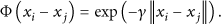
\begin{matrix} Φ (x_{i} - x_{j}) = e x p (- γ ‖x_{i} - x_{j}‖) . \end{matrix}

(1)

Polynomial kernel is

\begin{matrix} Φ (x_{i} - x_{j}) = (1 + x_{i} \cdot x_{j}) . \end{matrix}

(2)

Sigmoid kernel is

\begin{matrix} Φ (x_{i} - x_{j}) = \tanh (k x_{i} \cdot x_{j} - δ) . \end{matrix}

(3)

This study employed LIBSVM [22] as a classifier and an RBF as its kernel function, due to the ability of RBFs to handle nonlinear cases using fewer hyperparameters than that required for the polynomial kernel [23]. The SVM is regarded as a black box that receives input data and thereby builds up a classifier.

2.2. Cat Swarm Optimization (CSO)

CSO is a newly developed algorithm based on the behavior of cats, comprising two search modes: seeking and tracing. Seeking mode is modeled on a cat's ability to remain alert to its surroundings, even while at rest; tracing mode emulates the way that cats trace and catch their targets. These modes are used to solve optimization problems.

In CSO, every cat in a given population is given a position, velocity, and fitness value. Position represents a point corresponding to a possible solution set. Velocities are a variance of distance in a D-dimensional space. Fitness values refer to the quality of the solution set.

In every generation, CSO randomly distributes cats into either seeking mode or tracing mode, by which the position of each cat is then altered. Finally, the best solution set is indicated by the position of the cat with the highest fitness value.

2.2.1. CSO Process

The mixture ratio (MR) represents the percentage of cats distributed to tracing mode (e.g., if the total number of cats is 50 and value of MR is 0.2, the number of cats assigned to tracing mode will be 10). Because the cats spend most of the time resting, the value of MR is small. The process is outlined as follows. (1)

Randomly initialize N cats with position and velocities within a D-dimensional space.

(2)

Distribute cats to tracing or seeking mode; the number of cats in the two modes determines MR.

(3)

Measure the fitness value of each cat.

(4)

Search for each cat according to its mode in each iteration. The processes involved in these two modes are described in the following subsection.

(5)

Stop the algorithm if terminal criteria are satisfied; otherwise return to (2) for the following iteration.

Pseudocode 1 presents the pseudocode used in the main processes of CSO.

Pseudocode 1: Pseudocode of CSO.

Random initialize cats.

WHILE (is terminal condition reached)

Distribute cats to seeking/tracing mode.

FOR ( $i = 0$ ; i < NumCat; i++)

Measure fitness for cat $_{i}$ .

IF (cat $_{i}$ in seeking mode) THEN

Search by seeking mode process.

ELSE

Search by tracing mode process.

END

End FOR

End WHILE

Output optimal solution.

2.2.2. Seeking Mode

Seeking mode has four operators: seeking memory pool (SMP), self-position consideration (SPC), seeking range of the selected dimension (SRD), and counts of dimension to change (CDC). SMP defines the pool size of seeking memory. For example, an SMP value of 5 indicates that each cat is capable of storing 5 solution sets as candidates. SPC is a Boolean value, such that if SPC is true, one position within the memory will retain the current solution set and not be changed. SRD defines the maximum and minimum values of the seeking range, and CDC represents the number of dimensions to be changed in the seeking process. The process of seeking is outlined as follows. (1)

Generate SMP copies of the position of the current cat. If SPC is true, one of the copies retains the position of the current cat and immediately becomes a candidate. The other cats must be changed before becoming candidates. Otherwise, all SMP copies will perform searching resulting in changes in their positions.

(2)

Each copy to be changed randomly changes position by altering the CDC percent of dimensions. First, select the CDC percent of dimensions. Every selected dimension will randomly change to increase or decrease the current value of the SRD percent. After being changed, the copies become candidates.

(3)

Calculate the fitness value of each candidate via the fitness function.

(4)

Calculate the probability of each candidate being selected. If all candidate fitness values are the same, then the selected probability ( $P_{i}$ ) is equal to one. Otherwise, $P_{i}$ is calculated via (4). Variable i is between 0 and SMP; $P_{i}$ is the probability that this candidate will be selected; ${FS}_{\max}$ and ${FS}_{\min}$ represent the maximum and minimum overall fitness values; and ${FS}_{i}$ is the fitness value of this candidate. If the goal is to find the solution set with the maximum fitness value, then ${FS}_{b} = {FS}_{\min}$ ; otherwise ${FS}_{b} = {FS}_{\max}$ . Calculating probability using this function gives the better candidate a higher chance of being selected, and vice versa, as follows:

\begin{matrix} P_{i} = \frac{|{FS}_{i} - {FS}_{b}|}{{FS}_{\max} - {FS}_{\min}} . \end{matrix}

(4)

(5)

Randomly select one candidate according to the selected probability ( $P_{i}$ ). Once the candidate has been selected, move the current cat to this position.

2.2.3. Tracing Mode

Tracing mode represents cats tracing a target, as follows. (1)

Update velocities using (5).

(2)

Update the position of the current cat, according to (6) as follows:

\begin{array}{l} v_{k, d}^{t + 1} = v_{k, d}^{t} + r_{1} \times c_{1} \times (x_{b e s t, d}^{t} - x_{k, d}^{t}), \\ d = 1,2, \dots, D, \end{array}

(5)

\begin{array}{l} x_{k, d}^{t + 1} = x_{k, d}^{t} + v_{k, d}^{t} . \end{array}

(6)

$x_{k, d}^{t}$ and $v_{k, d}^{t}$ are the position and velocities of current cat k at iteration $t \cdot x_{b e s t, d}^{t}$ denotes the best solution set from ${c a t}_{k}$ in the population. $c_{1}$ is a constant and $r_{1}$ is a random number between 0 and 1.

3. Proposed MCSO-SVM

Neither seeking nor tracing mode is capable of retaining the best cats; however, performing a local search near the best solution sets can help in the selection of better solution sets. This paper proposes a modified cat swarm optimization method (MCSO) to improve searching ability in the vicinity of the best cats. Before examining the process of the algorithm, we must examine a number of relevant issues.

3.1. Classifiers

Classifiers are algorithms used to train data for the construction of models used to assign unknown data to the categories in which they belong. This paper adopted an SVM as a classifier. SVM theory is derived from statistical learning theory, based on structural risk minimization. SVMs are used to find a hyperplane for the separation of two groups of data. This paper regards the SVM as a black box that receives training data for the classification model.

3.1.1. Solution Set Design

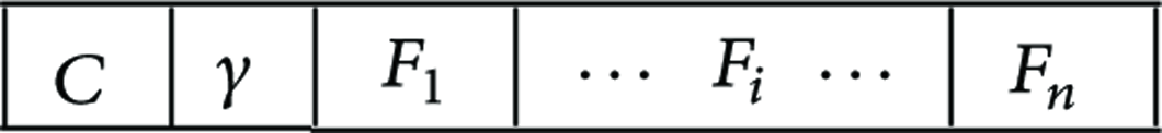
Figure 2 presents a solution set containing data in two parts: SVM parameters (C and γ) and feature subset. Parameter C is the penalty coefficient that means tolerance for error. And, parameter γ is a kernel parameter of RBF, which means radius of RBF. The continuous value of these two parameters will be converted into binary coding. Another is feature subset variables ( $F_{1} ~ F_{n}$ ) where n is the number of features. The range of the variables in each feature subset falls between 0 and 1. If $F_{i}$ is greater than 0.5, its corresponding feature is selected; otherwise, the corresponding feature is not chosen.

Figure 2

Representation of a solution set.

3.1.2. Mutation Operation

Mutation operators are used to locate new solution sets in the vicinity of other solution sets. When a solution set mutates, every feature has a chance to change. Figure 3 presents an example of mutation. Before the process of mutation, the first, second, and fourth features of the solution set were assigned for mutation; therefore, these features will be converted from selected 0.8(1) to unselected (0), unselected 0.3(0) to selected (1), and selected 0.9(1) to unselected (0). This operation is used only for the best solution sets; therefore, it is not necessary to maintain the actual position—recording the selected features is sufficient.

Figure 3

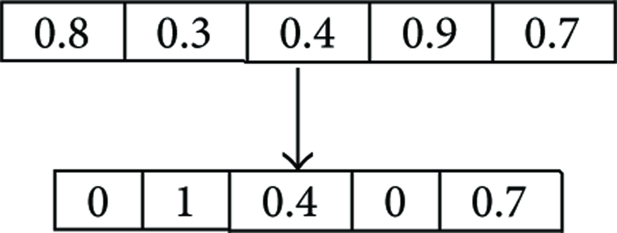
An example of mutation.

In addition, C and γ must be changed to binary, so they can select a mutation operation for the following search.

3.1.3. Evaluating Fitness

This study employed k-fold cross-validation [24] to test the search ability of the algorithms. k was set to 5, indicating that 80% of the original data was randomly selected as training data and the remainder was used as testing data. And then retain features up to a solution set that we want to evaluate for training data and testing data. This training data is input into an SVM to build a classification model used for the prediction of testing data. The prediction accuracy of this model represents its fitness.

In order to compare solution sets with the same fitness, we considered the number of selected features. If prediction accuracy were the same, the solution set with fewer selected features would be considered superior.

3.1.4. Proposed MCSO Approach

The steps of the proposed MCSO-SVM are presented as follows. (1)

Randomly generate N solution sets and velocities with D-dimensional space, represented as cats. Define the following parameters: seeking memory pool (SMP), seeking range of the selected dimension (SRD), counts of dimension to change (CDC), mixture ratio (MR), number of best solution sets (NBS), mutation rate for best solution sets (MR_Best), and number of trying mutation (NTM).

(2)

Evaluate the fitness of every solution set using SVM.

(3)

Copy the NBS best cats into best solution set (BSS).

(4)

Assign cats to seeking mode or tracing mode based on MR.

(5)

Perform search operations corresponding to the mode (seeking/tracing) assigned to each cat.

(6)

Update the BSS. For every cat after the searching process, if it is better than the worst solution set in BSS, then replace the worst solution set with the better solution set.

(7)

For each solution set in BSS, search by mutation operation for NTM times. If it is better than the worst solution set in BBS, then replace the worse solution set with the better solution set.

(8)

If terminal criteria are satisfied, output the best subset; otherwise, return to (4).

Figure 4 presents a flow chart of MCSO. The bold area indicates the processes added for the modification of CSO, while the other processes run as CSO. After searching in accordance with seeking and tracing modes, the cats with higher fitness can be updated to the best solution set (BSS). A mutation operation is then applied to BSS to search other solution sets. If a solution set following mutation shows improvement, it replaces the original solution set in the BSS.

Figure 4

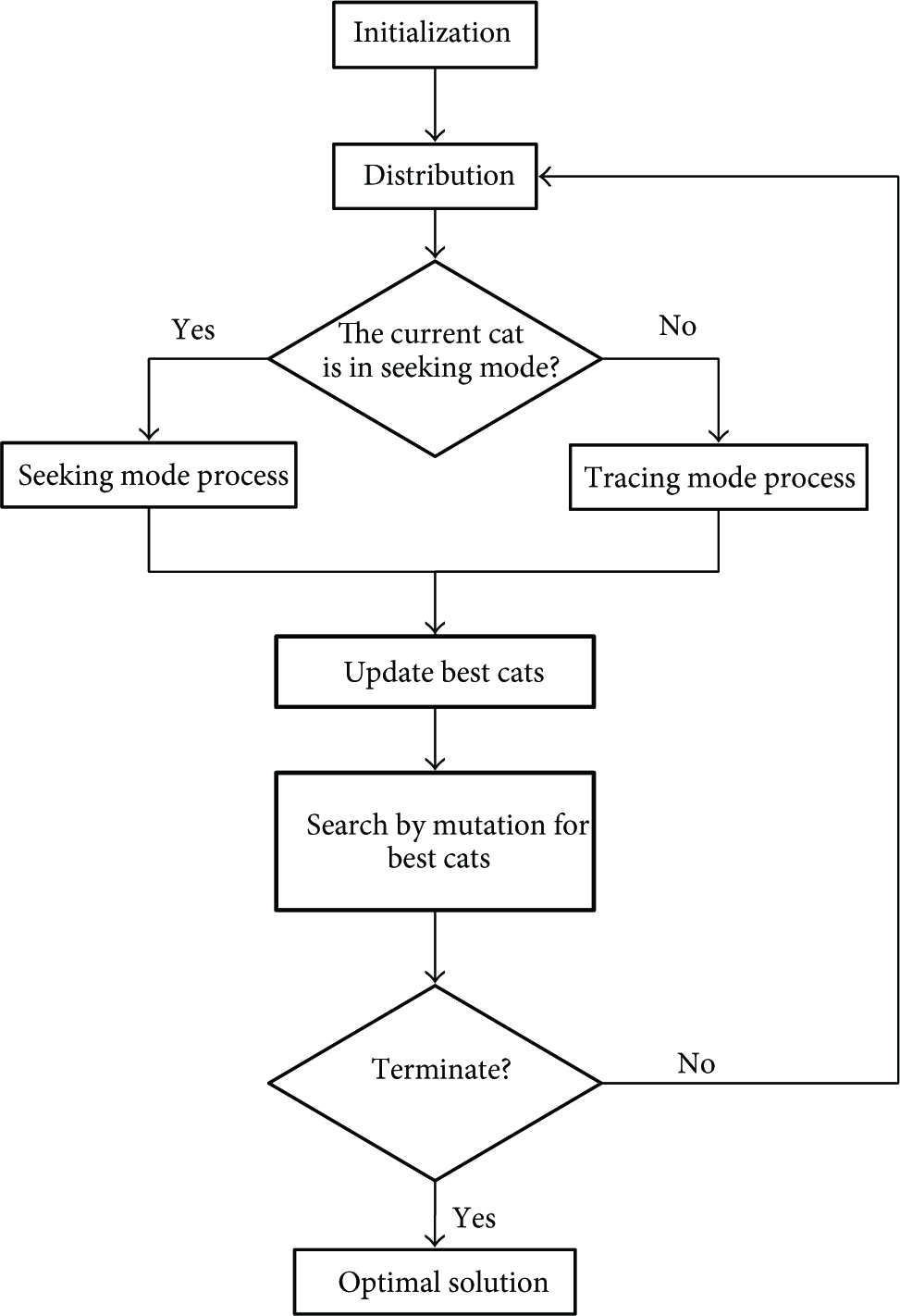
Flow chart of MCSO.

4. Experimental Results

This study followed the convention of adopting UCI datasets [20] to measure the classification accuracy of the proposed MCSO-SVM method. Table 1 displays the datasets employed.

Table 1

Datasets from UCI repository.

Number	Dataset	Number of classes	Number of features	Number of instances
1	Australian	2	14	690
2	Bupa	2	6	345
3	German	2	24	1000
4	Glass	6	9	214
5	Ionosphere	2	34	351
6	Pima	2	8	768
7	Vehicle	4	18	846
8	Vowel	11	10	528
9	Wine	3	13	178

The experimental environment was as follows: desktop computer running Windows 7 on an Intel Core i5-2400 CPU (3.10 GHz) with 4 GB RAM. Dev C++ 4.9.9.2 was used in conjunction with LIBSVM for development and a radial basis function (RBF) as the SVM kernel function.

Table 2 lists the parameter values used in the experiment. The terminal condition was determined as the inability to identify a solution set with higher classification accuracy, despite continuous iteration. We employed 5-fold cross-validation; that is, all values were verified five times to ensure the reliability of the experiment. The dataset was randomly separated into 5 segments. In each iteration, one segment was selected as test data (nonrepetitively) and the others were used as training data. The five tests were averaged to obtain a value of classification accuracy.

Table 2

Parameters of MCSO.

Parameter	N	SMP	SRD	CDC	MR	$c_{1}$	C	γ
Value or range	40	5	0.6	80%	20%	2	[0.01, 1024]	[0.00001, 8]

4.1. Experiment Parameters

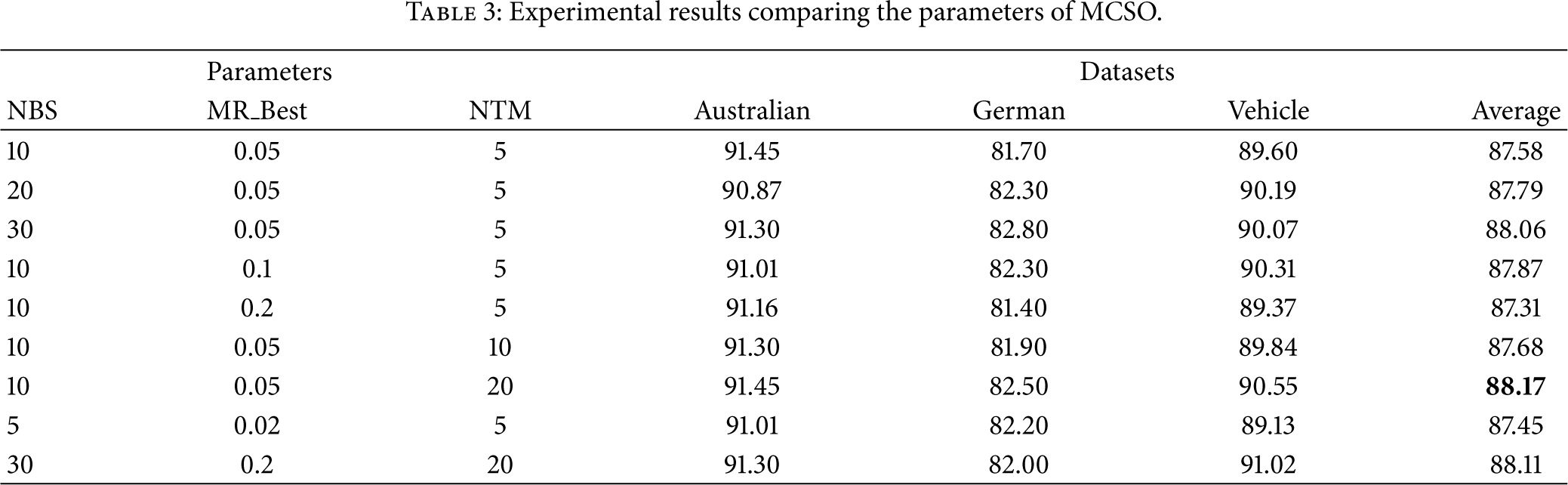
Various experiments were employed to test the parameters of the MCSO-SVM, including NBS, MR_Best, and NTM in nine groups. Table 3 lists the experimental results comparing the nine groups of parameters. The highest average classification accuracy for the three datasets was obtained using the following parameters: $N B S = 10$ , $M R_B e s t = 0.05$ , and $N T M = 20$ .

Table 3

Experimental results comparing the parameters of MCSO.

Parameters			Datasets
NBS	MR_Best	NTM	Australian	German	Vehicle	Average
10	0.05	5	91.45	81.70	89.60	87.58
20	0.05	5	90.87	82.30	90.19	87.79
30	0.05	5	91.30	82.80	90.07	88.06
10	0.1	5	91.01	82.30	90.31	87.87
10	0.2	5	91.16	81.40	89.37	87.31
10	0.05	10	91.30	81.90	89.84	87.68
10	0.05	20	91.45	82.50	90.55	88.17
5	0.02	5	91.01	82.20	89.13	87.45
30	0.2	20	91.30	82.00	91.02	88.11

4.2. Comparison with CSO-SVM

The best combination of nine parameters was applied in the comparison of CSO and MCSO. The results are presented in Table 4.

Table 4

Comparison results for CSO-SVM and MCSO-SVM.

Datasets	Number of original features	CSO-SVM		MCSO-SVM
Datasets	Number of original features	Number of selected features	Average accuracy rate (%)	Number of selected features	Average accuracy rate (%)
Australian	14	5.0	90.87	5.0	91.45^**
Bupa	6	3.8	79.13	4	79.42^**
German	24	6.6	80.00	8.2	82.50^**
Glass	9	4.4	83.65	4.2	84.60^***
Ionosphere	34	7.2	99.72	7.2	100^**
Pima	8	4.6	81.25	3.6	81.78^***
Vehicle	18	7.8	86.41	10.2	90.55^**
Vowel	10	7.8	100	7	100^*
Wine	13	3	100	2.8	100^*

$^{*}$ Accuracy is equal to the other method; however, fewer features are selected.

^**Higher accuracy.

^***Higher accuracy and fewer features are selected.

Table 4 compares MCSO-SVM and CSO-SVM with regard to classification accuracy and the number of selected features. For Glass and Pima datasets, the MCSO-SVM had higher classification accuracy and fewer selected features than CSO-SVM. In Australian, Bupa, German, Ionosphere, and Vehicle datasets, MCSO-SVM had higher classification accuracy. Due to the advantages afforded by searching in the vicinity of the best solution sets, MCSO-SVM clearly outperformed CSO-SVM.

Training time is a crucial issue in many situations, such that the best solution set is sacrificed for one that is good enough. The above experiment was used to illustrate the relationship between time and classification accuracy in CSO and MCSO, using the nine datasets described in Table 1, as shown in Figures 5 and 6. The horizontal axis represents the execution of processes (in seconds) while the vertical axis presents classification accuracy. MCSO appears in the upper-left corner of Figures 5 and 6, indicating that it takes less time to obtain results of higher accuracy. So, the MCSO is suitable for the real-world big data applications.

Figure 5

Relationship between time and classification accuracy using CSO and MCSO (Australia, Bupa, German, Glass, Ionosphere, and Pima).

Figure 6

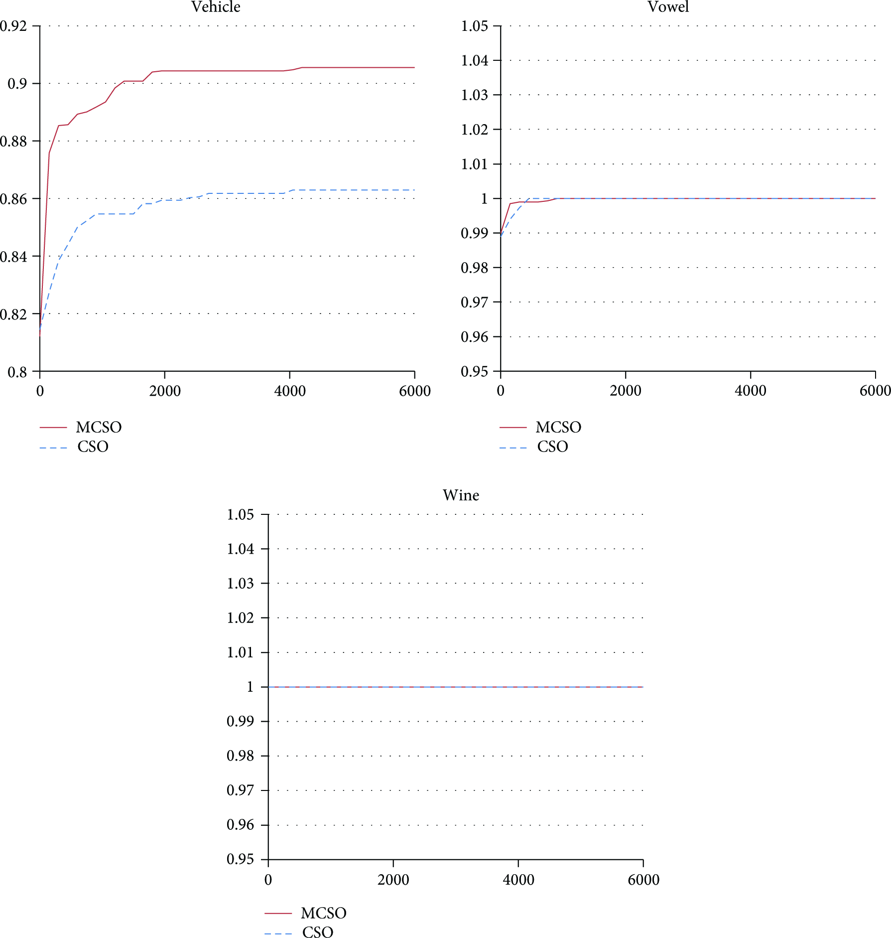
Relationship between time and classification accuracy using CSO and MCSO (Vehicle, Vowel, and Wine).

5. Conclusions

This study developed a modified version of CSO (MCSO) to improve searching ability by concentrating searches in the vicinity of the best solution sets. We then combined this with an SVM to produce the MCSO-SVM method of feature selection and SVM parameter optimization to improve classification accuracy. Evaluation using UCI datasets demonstrated that the MCSO-SVM method requires less time than CSO-SVM to obtain classification results of superior accuracy.

Footnotes

Conflict of Interests

The authors declare that there is no conflict of interests regarding the publication of this paper.

References

Holland

J. H.

Adaptation in Natural and Artificial Systems 1975

Ann Arbor, Mich, USA

The University of Michigan Press

MR0441393

Kennedy

Eberhart

Particle swarm optimization

Proceedings of the IEEE International Conference on Neural Networks

December 1995

Perth, Australia

1942 1948

2-s2.0-0029535737

X.-L.

Shao

Z.-J.

Qian

J.-X.

Optimizing method based on autonomous animats: fish-swarm Algorithm

System Engineering Theory and Practice 2002 22 11 32 38

2-s2.0-0036881676

Ishiguro

Kondo

Watanabe

Uchikawa

Shirai

Emergent construction of artificial immune networks for autonomous mobile robots

Proceedings of the IEEE International Conference on Systems, Man, and Cybernetics

October 1997

1222 1228

2-s2.0-0031360313

Kim

Gen

Kim

Adaptive genetic algorithms for multi-recource constrained project scheduling problem with multiple modes

International Journal of Innovative Computing, Information and Control 2006 2 1 41 49

Guo

Tian

Z.-H.

T.-B.

A lightweight web server anomaly detection method based on transductive scheme and genetic algorithms

Computer Communications 2008 31 17 4018 4025

10.1016/j.comcom.2008.08.009

2-s2.0-55049131898

M.-Y.

Real-time anomaly detection systems for Denial-of-Service attacks by weighted k-nearest-neighbor classifiers

Expert Systems with Applications 2011 38 4 3492 3498

10.1016/j.eswa.2010.08.137

2-s2.0-78650707301

Lin

K.-C.

Chen

S.-Y.

Hung

J. C.

Botnet detection using support vector machines with artificial fish swarm algorithm

Journal of Applied Mathematics 2014 2014 9

986428

10.1155/2014/986428

2-s2.0-84901045102

Lin

K. C.

Huang

T.-C.

Hung

J. C.

Yen

N. Y.

Chen

S. J.

Facial emotion recognition towards affective computing-based learning

Library Hi Tech 2013 31 2 294 307

10.1108/07378831311329068

2-s2.0-84879904018

10.

Chu

S. C.

Tsai

P. W.

Computational intelligence based on the behavior of cats

International Journal of Innovative Computing, Information and Control 2007 3 1 163 173

2-s2.0-48249095357

11.

Stevens

Goble

Baker

Brass

A classification of tasks in bioinformatics

Bioinformatics 2001 17 2 180 188

10.1093/bioinformatics/17.2.180

2-s2.0-0035098963

12.

Kishore

J. K.

Patnaik

L. M.

Mani

Agrawal

V. K.

Application of genetic programming for multicategory pattern classification

IEEE Transactions on Evolutionary Computation 2000 4 3 242 258

10.1109/4235.873235

2-s2.0-0034266799

13.

Furey

T. S.

Cristianini

Duffy

Bednarski

D. W.

Schummer

Haussler

Support vector machine classification and validation of cancer tissue samples using microarray expression data

Bioinformatics 2000 16 10 906 914

10.1093/bioinformatics/16.10.906

2-s2.0-0033636139

14.

Zhang

G. P.

Neural networks for classification: a survey

IEEE Transactions on Systems, Man and Cybernetics Part C: Applications and Reviews 2000 30 4 451 462

10.1109/5326.897072

2-s2.0-0034313673

15.

Quinlan

J. R.

C4.5: Programs for Machine Learning 1993

San Francisco, Calif, USA

Morgan Kaufmann

16.

Liu

Motoda

Feature Selection for Knowledge Discovery and Data Mining 1998

Springer

17.

C. J.

Chuang

L.-Y.

Chang

J.-Y.

Yang

C.-H.

Feature selection using PSO-SVM

Proceedings of the International Multiconference of Engineers and Computer Scientists (IMECS ′06)

2006

138 143

18.

Lin

K.-C.

Chien

H.-Y.

CSO-based feature selection and parameter optimization for support vector machine

Proceedings of the Joint Conferences on Pervasive Computing (JCPC ′09)

December 2009

Taipei City, Taiwan

783 788

10.1109/JCPC.2009.5420080

2-s2.0-77951263656

19.

Lin

K.-C.

Huang

Y.-H.

Hung

J. C.

Lin

Y.-T.

Modified cat swarm optimization algorithm f or feature selection of support vector machines

Frontier and Innovation in Future Computing and Communications 2014 301 329 336 Lecture Notes in Electrical Engineering

20.

Hettich

Blake

C. L.

Merz

C. J.

UCI Repository of Machine Learning Databases

1998, http://www.ics.uci.edu/~mlearn/MLRepository.html

21.

Vapnik

V. N.

The Nature of Statistical Learning Theory 1995

New York, NY, USA

Springer

MR1367965

22.

Chang

C.-C.

Lin

C.-J.

LIBSVM: a library for support vector machines

2011, http://www.csie.ntu.edu.tw/~cjlin/libsvm

23.

Hsu

C. W.

Chang

C. C.

Lin

C. J.

A Practical Guide to Support Vector Classication 2003 http://www.csie.ntu.edu.tw/~cjlin/papers/guide/guide.pdf

24.

Salzberg

S. L.

On comparing classifiers: pitfalls to avoid and a recommended approach

Data Mining and Knowledge Discovery 1997 1 3 317 328

10.1023/A:1009752403260

2-s2.0-27144463192

Feature Selection and Parameter Optimization of Support Vector Machines Based on Modified Cat Swarm Optimization

Abstract

1. Introduction

2. Related Work

2.1. Support Vector Machine (SVM)

2.2. Cat Swarm Optimization (CSO)

2.2.1. CSO Process

Pseudocode 1: Pseudocode of CSO.

2.2.2. Seeking Mode

2.2.3. Tracing Mode

3. Proposed MCSO-SVM

3.1. Classifiers

3.1.1. Solution Set Design

3.1.2. Mutation Operation

3.1.3. Evaluating Fitness

3.1.4. Proposed MCSO Approach

4. Experimental Results

4.1. Experiment Parameters

4.2. Comparison with CSO-SVM

5. Conclusions

Footnotes

Conflict of Interests

References