Sage Journals: Discover world-class research

Abstract

This paper tackles the coverage problem in homogenous and heterogeneous wireless sensor networks. The homogenous sensor network consists of sensor nodes and relays; however, the heterogeneous sensor network consists of sensor nodes, super nodes, and satellite nodes. In the latter network, super nodes and satellite nodes are utilized to demonstrate different scenarios. Super nodes consume huge amount of energy, compared to sensor nodes. To address this problem, the aim of this paper is to find the baseline when super nodes are used efficiently, despite the inherited high power consumption. Wolfram Mathematica is used to compare random independent deployment circular analytical model against a much simpler square analytical model. The achieved results showed that the simple square model is very close to circular model when K-coverage is ≤2.

1. Introduction

Deploying wireless sensors in a region to cover the entire area of interest is one of the main research issues in wireless sensor networks (WSN) [1–3]. Coverage of an area is determined by the quality of the sensing capabilities of the sensors; however, coverage definition is dependent on applications [4]. Different solutions are affected and constrained by sensors' sizes, weights, and costs. More important is the impact of network connectivity due to energy constraint. Currently, replacing batteries is not feasible so most applications are designed to be energy aware. Normally, energy conservation is implemented in both hardware and software. As a result, many algorithms and protocols are designed and implemented to minimize power consumption [5–8]. Moreover, major improvement can be done to reduce the energy consumption of super nodes (SNs). The lifetime of a sensor network on average is one year [5]. A wireless sensor network (WSN) is considered alive for that period which can collect data from sensors to the gateway. Moreover, many of the wireless sensor networks exhibit deterministic node deployment. This makes it one of the main objectives, which is minimizing the number of sensors [6, 9]. If every point in the area of the network is monitored by no less than k distinct sensors, the WSN is considered to be K-covered [7, 10, 11]. To prolong the lifetime and minimize energy consumption, sleep-scheduling approaches are used [5, 12–15]. The topology of the network also affects the power consumption of the sensors and consequently the lifetime of the network. In this paper, a cluster-based network is used to compare homogenous and heterogeneous networks. Two WSN scenarios are demonstrated, one scenario is with gateways and, in the other scenario, the WSN is mixed with SNs. In the first scenario, cluster heads are selected in such a way to minimize the energy consumption of the WSN all in all. A mechanism to optimize the sensing coverage is proposed [16]. In this proposal the authors discussed the hybrid problem; however, the WSN is not fully covered all the time. An energy-efficient heuristic to maximize total network lifetime is proposed in [17]. In an experimental setup, the authors compared the performance of two protocols, greedy [18] and High-Energy-First (HEF) [19], against the maximum coverage heuristic (MCH). The authors did not handle K-coverage problem and also did not describe whether the network is alive.

In this paper, the focus is on network connectivity with different levels of coverage, which means each active sensor can communicate with base station/super node and other active sensor nodes. We also simplify the traditional circular model with a square model, which makes the analysis of the coverage problem much easier. Moreover, we integrate the SNs that have the ability to communicate directly with satellite nodes to improve the quality of coverage. We run different scenarios to test the performance of the system and finally we compare the two-tier system with the regular wireless sensor network in terms of K-coverage and energy consumption.

In Section 2, we discuss randomized independent scheduling model, describe the random uniform distribution of the system, and compare the circular model against the square model. In Section 3, we describe the triggering mechanism of the network to collect information and show the distribution and the coverage of the sensors. In Section 4, we show detailed power calculations for each step in the system.

2. Randomized Independent Scheduling Model

In this section, we compare the square model with Kumar's random analytical deployment [5]. To calculate the coverage, circles are replaced by squares to calculate the sensing range of sensors. This model is much easier than the traditional circular model. We would like to find the limitations of the square model and set a baseline where it can be used. Moreover, Wolfram Mathematica package is utilized to implement Kumar's circular model and compare the outcomes against Kumar's original results. We start by defining the parameters to be used in the square model: (i)

n is the number of nodes in the field.

(ii)

p is the likelihood that a sensor is active.

(iii)

r is sensing range.

(iv)

Growth function: a function $ϕ (n p)$ is slowly growing if it is monotonically increasing and approaches infinity as $n \to \infty$ with $O (\log (\log (n p)))$ .

(v)

Let $g (x) = o (f (x)) i f f \lim_{x \to \infty} (g (x) / f (x)) = 0$ , $g (x) = ω (f (x)) i f f \lim_{x \to \infty} (g (x) / f (x)) = \infty$ , and $g (x) \approx f (x) i f f \lim_{x \to \infty} (g (x) / f (x)) = 1$ .

(vi)

Let the coverage function $c (n) = n p π r^{2} / l o g (n p)$ .

(vii)

For each point $u \in L$ , let $A (u)$ denote the event where u is covered and $\bar{A (u)}$ is its negation.

(viii)

$E (x)$ = expected value.

(ix)

$ϕ^{'} (n p) = ϕ (n p) - o (c (n))$ .

(a)

$N_{r} (u)$ denotes the number of active sensors in $D_{r} (u)$ , and probability that active sensors are equal to i is $P_{i} (u) = P_{r} [N_{r} (u) = i]$ .

(x)

$D_{r} (u)$ is a circle with radius r centered at point u.

The investigation starts by showing that if a definite (limited) set of objects in the unit square is K-covered by a WSN with a definite sensing coverage then subsequently the full space is K-covered by an equivalent network with a larger sensing range. All utilized nodes are referred to by L which are the points in $\sqrt{l} \times \sqrt{l}$ virtual network on the unit square area as delineated in Figure 1. With this outcome, it is possible to show the unit square is K-covered using a suitable value of l. Figure 1 shows a square grid contains 169 objects (13 × 13).

Figure 1

A virtual unit square area grid overlaid with 169 objects.

2.1. Random Uniform Distribution

We discuss the random distribution of (in)active sensor. In this distribution, sensors are placed systematically over the virtual grid as shown in Figure 2. This figure provides an example of 300 nodes that are randomly distributed with probability of 0.1. Please note that, at any point in the grid, sensors have an equivalent probability distribution.

Figure 2

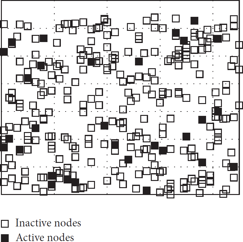
Random distribution of 400 nodes with probability = 0.1.

We calculate the coverage function by number of sensors with a certain probability of being active.

2.1.1. Statement

Let a number of sensors, n, be distributed uniformly in virtual square grid. If the function is monotonically increasing and approaches infinity as the number of nodes is large and p and r are satisfied, then coverage function $c (n)$ is as follows:

\begin{matrix} c (n) \geq 1 + \frac{ϕ (n p) + k \log (\log (n p))}{\log (n p)}, \end{matrix}

(1)

where k is the number of active sensors and p is the probability that a sensor is active. For a detailed proof of this formula, please refer to our previous work in [20].

2.1.2. The Proposed Square Model

We swap the circular model with a square model (Figure 3). The circular model is similar to the square model, however the coverage function of the square model is: $c (n) = n p (2 r)^{2} / l o g (n p)$ .

Figure 3

Area of a square against a circle.

For a detailed proof of this formula, please refer to our previous work in [20].

3. Simulation Model

To demonstrate the experimental results on different scenarios, a custom made simulator is developed using Java to simulate K-coverage with random deployment. The amount of sensors required for each coverage level is calculated and the results are compared against the analytical model utilizing the same parameters.

Kumar et al. [5] simulated the random deployment. At the beginning, the aim is to make sure that the achieved results are similar to those achieved by Kumar's model and then the proposed square model is investigated. During these experiments, scheduling the WSN via SN is studied and we compare the performance of power consumption, K-coverage, and delay with random deployment. We name satellite with WSN as Satellite Wireless Sensor Network (SWSN).

In this simulation, sensors are randomly distributed in a 100 × 100 unit grid. Sensors are active with probability p and are switched off otherwise. The sensing range $R_{s}$ is the same for all sensors with 1.5u; however, the communication range $R_{c}$ is double sensing range with $R_{c} = 2 R_{s}$ . SNs are used as relays and their $R_{c}$ is equivalent to normal sensors. The number of nodes is increased gradually to evaluate K-coverage with different densities. The most optimized scenario is that every node senses five grid cells without intersecting with other nodes. If we require the WSN to work ten times as much as that covered in the best scenario, then we need to cover every 5 cells with ten nodes at minimum. As a result, the minimum number of sensors is 20,000 sensors (10 sensors × 10,000 cells)/5 cells.

In the simulation experiments, we take average of 100 runs and check the live sensors in each round.

The coverage of the two types of sensors is shown in Figure 4. Each sensor node covers five cells and each SN covers 13 cells.

Figure 4

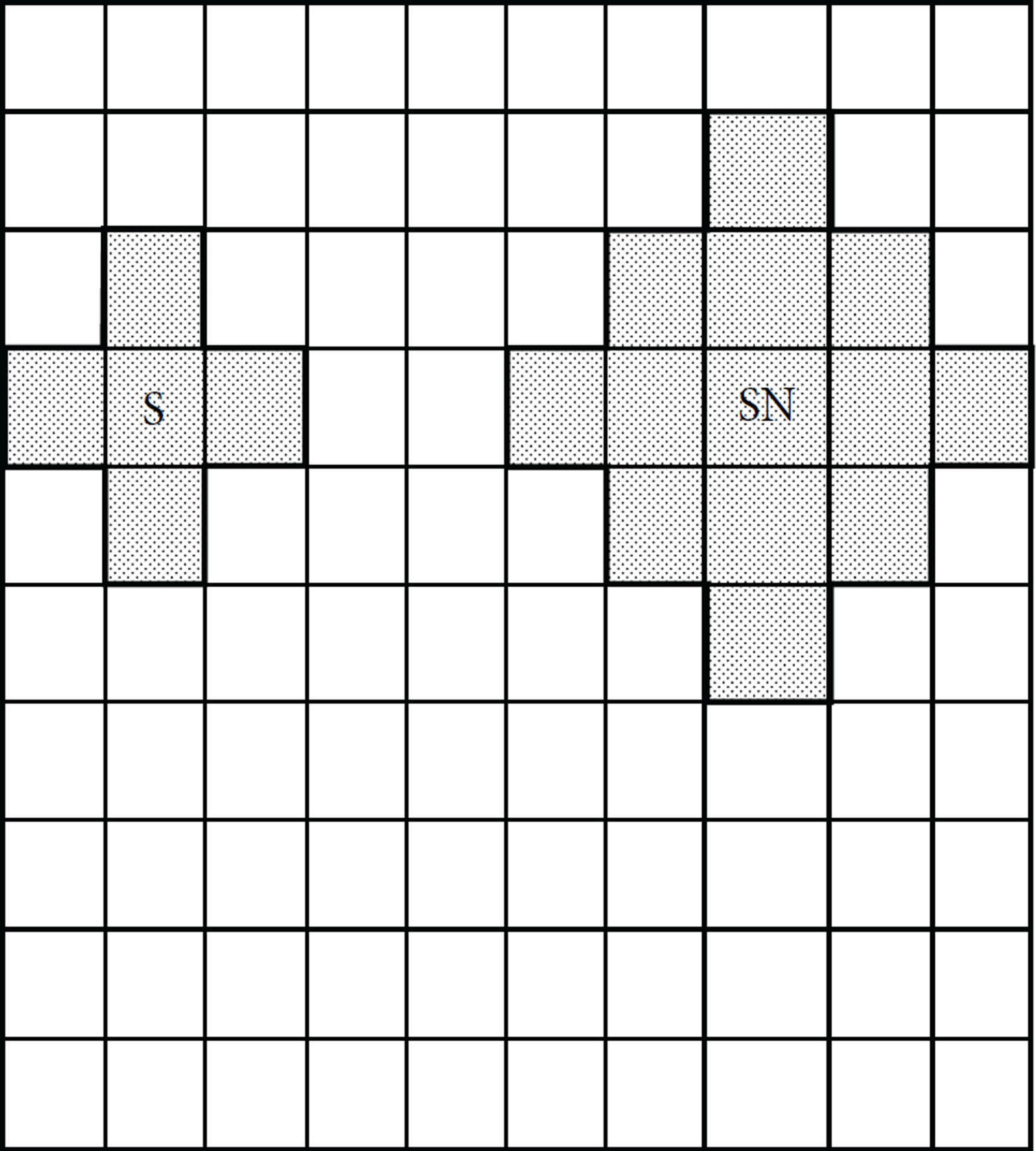
Sensing coverage of S and SN.

The parameters in Figure 5 are as follows: N is the number of sensors to be deployed, C is counter, and t is time.

Figure 5

Deployment process mechanism.

Different scenarios of network communication are performed for which the basis for calculating energy consumption of the network is derived. The trigger mechanisms and all phases of the procedure are depicted conceptually in Figures 6 and 7. Figure 6 depicts data collection scenario inquired by satellite. In Figure 6(a), the network is in the listening mode. The satellite triggers SN process of data collection by communicating a message to the SNs (Figure 6(b)). The SNs initiate messages to the sensor nodes to collect the required data (Figure 6(c)). In Figure 6(d), sensor nodes collect the required data. After that, sensor nodes communicate the data to SN (Figure 6(e)). Finally, SN sends the data to the satellite as shown in Figure 6(f).

Figure 6

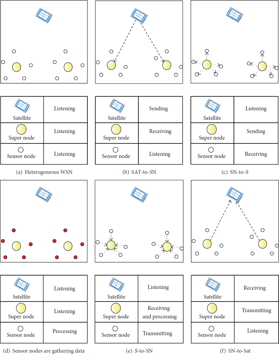
Satellite initiation query.

Figure 7

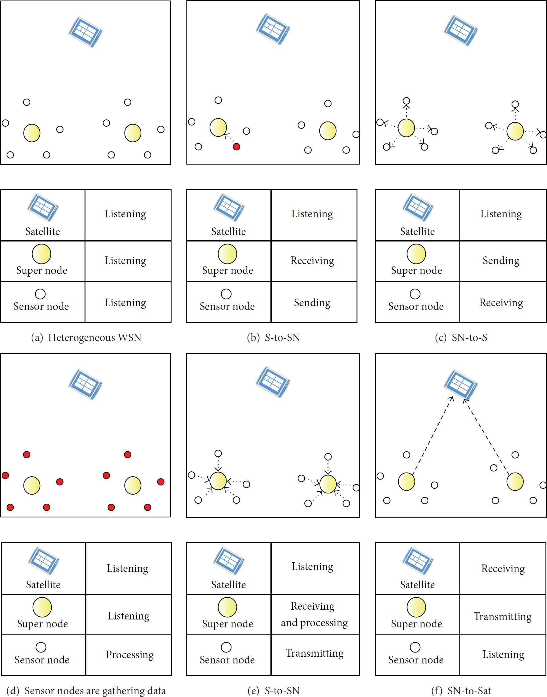
Periodic or event driven, initiated by sensors.

Figure 7 depicts data collection scenario for event-driven data scenario. In Figure 7(a), the network is in the listening mode. When a certain threshold is reached at one of the sensors, it triggers the process of data collection by communicating a message to the SN (Figure 7(b)). The SN sends message to the sensor nodes to inquire about the status of other sensor nodes (Figure 7(c)). In Figure 7(d), sensor nodes collect the required data. After the data is collected, sensor nodes communicate the data to SN (Figure 7(e)). Finally, that super node processes the data; if most/all the sensor nodes have reached the threshold, the data is sent to the satellite by SN (Figure 7(f)); otherwise no action is taken.

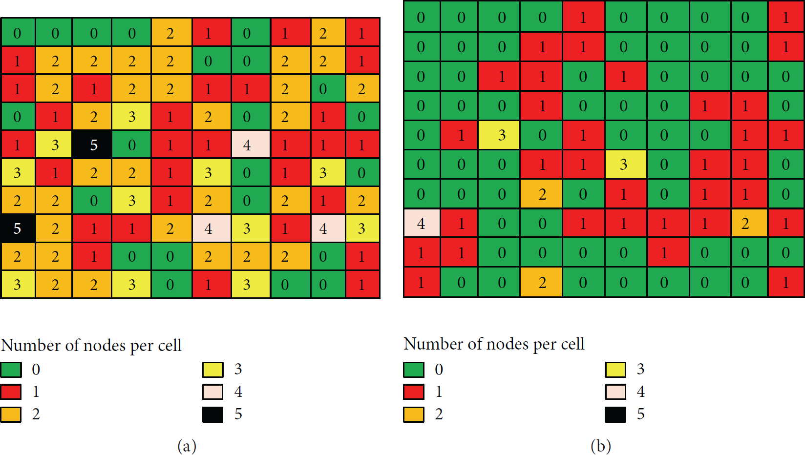
We demonstrate an example of the coverage concept for WSN and SN in Figure 8. In Figures 8(a) and 8(b), we show the location of randomly distributed sensors and super nodes, respectively, with $p = 0.1$ . There are 149 active sensors and 49 active SN in Figures 8(a) and 8(b), respectively. It is clear that the WSN model coverage is better than that of SN in terms of coverage due to the better distribution.

Figure 8

Location of active sensor and super nodes.

Figure 9 depicts a clearer distribution of the number of nodes per cell. We show the number of active sensors/SNs versus the number of cells. The WSN has a better distribution than that of SN due to the number of deployed nodes.

Figure 9

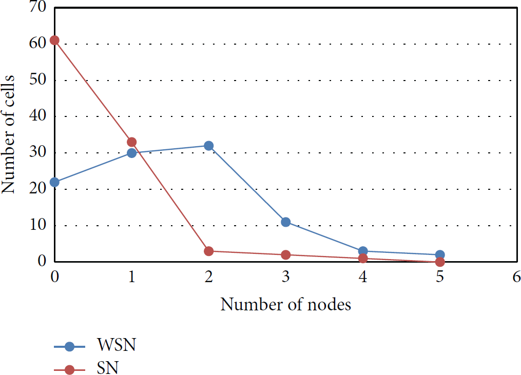
Nodes distribution per cell.

K-coverage for each cell is depicted in Figure 10. We start by K-coverage = 1 up to K-coverage = 13 and calculate the percentage of K-coverage for each case. The WSN has a better K-coverage than that of SN as a result of the better distribution.

Figure 10

K-coverage level in each cell.

In Figures 11 and 12, we find different levels of coverage, starting from $K 1$ up to $K 10$ , using the simulation model of WSN with and without SN models. As it can be seen from the results in Figures 11 and 12, they have the same trend; however, as expected, SN requires much less number of nodes for the same level of K-coverage.

Figure 11

Coverage using simulation model without using SN.

Figure 12

Coverage using simulation model using SN.

The results of the analytical models are compared against the simulation model in Figure 13. We notice that the square analytical model is close to the simulation results when $K = 1$ and 2. However, when $K > 2$ , the analytical model with a circle radius is similar to the simulation results in the range of 95–99%. This result supports the established results.

Figure 13

K-coverage of simulation and analytical model comparing.

Out of the simulation results, we observe that more than 50 sensors in active mode cover some cells at the same time. This causes loss of energy and interference. Organizing the deployment of the wireless sensors solves this problem. Alternative approaches to solve this problem are to use a sleep-scheduling mechanism such as Probing Environment and Adaptive Sensing [21, 22] or Maximization of Sensor Network Life (MSNL) [23].

4. Power Calculation

The triggering process starts by the satellite node. It triggers the network requesting data from the field. The comparison is made between the following two configurations: one with only normal sensors in the network and another with SN. The Global Positioning System (GPS) is a great technological success story [24, 25]. A comprehensive treatment of the system, signals, performance, and applications are in [26]. The SN utilizes the GPS technologies to communicate with satellites.

The number of deployed sensors is the same and they are adequate for 1-coverage. However, the number of active sensors is different each time because of the random distribution.

For the SN, the energy consumed in the transmission part is much higher than that between the sensors. For instance, the satellite networks in the Low Earth Orbit (LEO) that are in the range between 1414 and 3500 Km (Globalstar) consume approximately one watt of power and work with a low data rate [26]. It should be noted that, using one watt of power, a mobile phone could work for 120 hours in normal mode or about 4 hours of continuous voice use. In this simulation, the power consumed in communication with satellite is between 0.6 and 1 watt per transmission; however, communication between sensor nodes consumes 50 μW on average. In other words, each transmission to the satellite consumes as much power as 12,000–20,000 transmissions between nodes. We compare the power consumptions to find the threshold at which adding SN improves the network.

To calculate the power consumption in SWSN, the following formulas are utilized [13]:

\begin{matrix} E_{S N} = P_{r e c e i v . (S N \leftarrow S A T)} t_{r e c e i v . (S N \leftarrow S A T)} + P_{P r o c e s s (S N)} t_{P r o c e s s (S N)} + P_{t r a n s . (S N \to S A T)} t_{t r a n s . (S N \to S A T)} + P_{t r a n s . (S N \to S)} t_{t r a n s . (S N \to S)} + P_{r e c e i v . (S \to S N)} t_{r e c e i v . (S \to S N)}, \\ E_{S} = P_{r e c e i v . (S N \to S)} t_{r e c e i v . (S N \to S)} + P_{t r a n s . (S \to S N)} t_{t r a n s . (S \to S N)} + P_{s e n s . (S)} t_{s e n s . (S)} + P_{P r o c e s s . (S)} t_{P r o c e s s . (S)}, \\ E_{S c} = n_{s a} (P_{receiv . (S N \to S)} t_{receiv . (S N \to S)} + P_{trans . (S \to S N)} t_{trans . (S \to S N)} + P_{sens . (S)} t_{sens . (S)} + P_{Process . (S)} t_{Process . (S)}), \end{matrix}

(2)

where

E_{S N}

is energy consumed by each SN (sensor node) in each communication,

P_{r e c e i v . (S N \leftarrow S A T)}

is power consumed by SN for receiving request from the satellite,

t_{r e c e i v . (S N \leftarrow S A T)}

is amount of time taken for SN to receive request from the satellite,

P_{t r a n s . (S N \to S A T)}

is power consumed by SN for transmitting replay to the satellite,

P_{s e n s . (S)}

is power consumed by S for sensing function,

E_{S c}

is the total consumed by the entire S node under the SN, and

n_{s a}

is the number of active sensors under the SN.

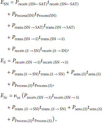
In the proposed model, we have the following assumptions: (1)

The energy consumed by satellite is not counted.

(2)

The required amount of energy per hop is equal to one energy unit.

On average, the energy consumption of SWSN is 50 times more than that of WSN. This is shown in Table 1.

Table 1

Average power consumption for 1-coverage.

Energy in WSN	Energy of SWSN
2,512,484	136,037,390

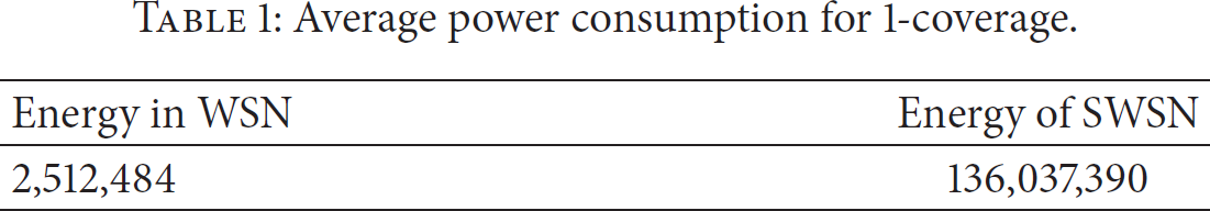
Figure 14 shows the relationship between the energy consumption and number of communications between satellite and SNs. An acceptable threshold for making an SN viable is found for the $100 * 100$ unit model when comparing the power consumed by S and SN. From Figure 14, when the power consumed by one communication to satellite is 290 times the cost of power consumption between two sensors, the use of the SN is feasible. However, this is not the case after testing the lower bound in random uniform distribution.

Figure 14

Finding the acceptable threshold for SWSN.

5. Comparison between the Two Systems

We conduct a performance comparison with the same working area, $100 * 100$ unit grid. In addition, at least 20,000 sensors with probability of 0.1 are needed to cover a ten thousand locations for 1-coverage; this gives 2000 (10000/5) active sensors.

If the data is sent to SNs or gateway in the corners of the grid, then the best case is one hop, while the worst case is 50 hops. Thus, the average is 25 hops. Assuming all sensors have data to send, the total hops for sending are equal to 50000 ( $2000 * 25$ ) energy units.

For a system with SNs, all of the sensors are one hop from the SN. In addition, each cell is covered by one sensor. Therefore, $2000 * 1$ equals 2000 energy units.

The cost of sending data from SNs to satellite is added. This is the number of SNs multiplied by 16,000 (the average of 12,000–20,000.)

From the above calculations, it is clear that the normal sensors in SWSN in the worst case scenario have longer lifetime by a factor of 25 times.

To clarify the idea, we provide another example with smaller grid.

Assuming $10 * 10$ grid, with 100 cells, we need 100/5 = 20 active sensors for 1-coverage. Without SN, each sensor communicates with the sink with an average of 5.5 energy unit. With SN, each sensor sends SN with average of one energy unit, that is, no change from the previous scenario.

This clearly shows that the power needed without SN is 5.5 times greater than that of SWSN provided that the communication to the satellite is ignored.

We find the effect of the increase in the size of covered area versus the energy consumed in both WSN and SWSN, as depicted in Figure 15.

Figure 15

Consumed energy of WSN versus SWSN.

From Figure 15, it is clear that the use of SN is not practical due to the huge amount of energy needed for sending data to satellite. However, if we use a continuous power source for SN, which is feasible in some applications, it may become an acceptable model.

In Figure 16, we ignore the energy consumed by the SN for communication with satellite. As a result, the energy consumed by WSN is increased exponentially. To take advantage of both SWSN and WSN, we suggest using the satellite to trigger the SNs. After that, the SNs trigger the sensors and the data is returned by the multihop WSN to the sink of the network.

Figure 16

Consumed energy of WSN versus SWSN versus new system.

This suggestion reduces the energy used in communication by 50 percent, which is an excellent improvement considering the only addition required is the SN.

6. Conclusion

In this paper, we compare one-tier versus two-tier wireless sensor networks coverage problem with different scenarios. We used the random independent deployment analytical model by Kumar and applied it in Mathematica program. We used a custom-made Java simulator to compare the results obtained against the ones by Mathematica. We introduced the square model for its simplicity and compared it against the conventional circular mode. The square analytical model is close to the simulation results when $K \leq 2$ . However, if $K > 2$ , the circular analytical model is much closer to the simulation results. We also investigated the energy consumption for each model to define a baseline, where the usage of SWSN is feasible. Finally, we introduced a new architecture to trigger the WSN by satellite and proved that it outperformers the regular WSN. Using the triggering mechanism in SWSN by satellite saves 50 percent of the energy consumed in communication. The limitation of the system is the power budget and availability of satellite nodes in the area. Moreover, the line of sight communication is another limitation. We can use SWSN in remote areas to connect the WSN to each other or to the main system. In addition, it is feasible if we connect the SNs to constant power supply. In the future, we can study different scheduling schemes triggered by satellite. In addition, another solution would be to use an unmanned aircraft to trigger the wireless sensor network and collect the data.

Footnotes

Conflict of Interests

The author declares that there is no conflict of interests regarding the publication of this paper.

Acknowledgment

The author would like to acknowledge the support of King Fahd University of Petroleum and Minerals (KFUPM) for this work.

References

Singh

Sharma

T. P.

A survey on area coverage in wireless sensor networks

Proceedings of the International Conference on Control, Instrumentation, Communication and Computational Technologies (ICCICCT ′14)

July 2014

Kanyakumari, India

IEEE

829 836

10.1109/iccicct.2014.6993073

2-s2.0-84921665798

Khan

M. A.

Hasbullah

Nazir

Khan

M. A.

Lifetime and coverage maximization technique for mobile sensor networks

Proceedings of the International Conference on Computer and Information Sciences (ICCOINS ′14)

June 2014

Kuala Lumpur, Malaysia

1 6

10.1109/iccoins.2014.6868394

Gong

Zhang

Chen

Sun

Curve-based deployment for barrier coverage in wireless sensor networks

IEEE Transactions on Wireless Communications 2014 13 2 724 735

10.1109/TWC.2013.121813.130198

2-s2.0-84896396765

Meguerdichian

Koushanfar

Potkonjak

Srivastava

M. B.

Coverage problems in wireless ad-hoc sensor networks

Proceedings of the 20th Annual Joint Conference of the IEEE Computer and Communications Societies (INFOCOM ′01)

April 2001

Anchorage, Alaska, USA

IEEE

1380 1387

10.1109/INFCOM.2001.916633

Kumar

Lai

T. H.

Balogh

On k-coverage in a mostly sleeping sensor network

Proceedings of the 10th Annual International Conference on Mobile Computing and Networking (MobiCom ′04)

October 2004

144 158

2-s2.0-11244289227

Cardei

Coverage in Wireless Sensor Networks, 2005

IEEE

IEEE standard for information technology—part 15.4: wireless medium access control (MAC) and physical layer (PHY) specifications for low rate wireless personal area networks (LR-WPANS)

IEEE 2003 802.15.4

Yang

Chen

Sun

Energy-efficient probabilistic area coverage in wireless sensor networks

IEEE Transactions on Vehicular Technology 2015 64 1 367 377

10.1109/TVT.2014.2300181

2-s2.0-84921358942

Chen

C.-P.

Mukhopadhyay

S. C.

Chuang

C.-L.

Lin

T.-S.

Liao

M.-S.

Wang

Y.-C.

Jiang

J.-A.

A hybrid memetic framework for coverage optimization in wireless sensor networks

IEEE Transactions on Cybernetics 2014

10.1109/TCYB.2014.2371139

10.

Liang

C.-K.

Tsai

C.-H.

M.-C.

On area coverage problems in directional sensor networks

International Conference on Information Networking (ICOIN ′11)

January 2011

182 187

10.1109/icoin.2011.5723175

2-s2.0-79952951280

11.

Ammari

H. M.

On the problem of k-coverage in 3d wireless sensor networks: a Reuleaux tetrahedron-based approach

Proceedings of the 7th International Conference on Intelligent Sensors, Sensor Networks and Information Processing (ISSNIP ′11)

December 2011

389 394

10.1109/issnip.2011.6146631

2-s2.0-84857925549

12.

Deng

Han

Y. S.

Heinzelman

W. B.

Varshney

P. K.

Scheduling sleeping nodes in high density cluster-based sensor networks

Mobile Networks and Applications 2005 10 6 825 835

13.

Wang

Topology-based routing for xmesh in dense wireless sensor networks [Ph.D. thesis] 2007

Stony Brook, NY, USA

Electrical Engineering, Stony Brook University

14.

Liang

Liu

Kui

A survey of coverage problems in wireless sensor networks

Sensors & Transducers 2014 163 1 240 246

2-s2.0-84896289466

15.

Abidin

H. Z.

Din

N. M.

Jalil

Y. E.

Multi-Objective Optimization (MOO) approach for sensor node placement in WSN

Proceedings of the 7th International Conference on Signal Processing and Communication Systems (ICSPCS ′13)

December 2013

1 5

10.1109/icspcs.2013.6723994

2-s2.0-84903830291

16.

Liao

Wang

Zhang

Cao

Min

Minimizing movement for target coverage and network connectivity in mobile sensor networks

IEEE Transactions on Parallel and Distributed Systems 2015 26 7 1971 1983

17.

Bajaj

Manju

Maximum coverage heuristics (MCH) for target coverage problem in Wireless Sensor Network

Proceedings of the 4th IEEE International Advance Computing Conference (IACC ′14)

February 2014

300 305

10.1109/iadcc.2014.6779338

2-s2.0-84899062481

18.

Cardei

Thai

M. T.

Energy-efficient target coverage in wireless sensor networks

Proceedings of the IEEE INFOCOM

March 2005

1976 1984

2-s2.0-25844504705

19.

Chaudhary

Pujari

A. K.

High-energy-first (HEF) heuristics for energy-efficient target coverage problem

International Journal of Ad Hoc, Sensor & Ubiquitous Computing 2011 2 1

20.

Sheltami

T. R.

Mahmoud

Alafari

Shakshuki

Self-organizing sensor networks: coverage problem

Proceedings of the 26th Biennial Symposium on Communications (QBSC ′12)

May 2012

Kingston, Canada

Queen's University

91 96

10.1109/QBSC.2012.6221358

21.

Tian

Georganas

N. D.

A coverage-preserving node scheduling scheme for large wireless sensor networks

Proceedings of the 1st ACM International Workshop on Wireless Sensor Networks and Applications (WSNA ′02)

September 2002

32 41

2-s2.0-0036983403

22.

Zhong

Cheng

Zhang

PEAS: a robust energy conserving protocol for long-lived sensor networks

Proceedings of the 23th IEEE International Conference on Distributed Computing Systems (ICDCS ′03)

May 2003

28 37

2-s2.0-0037630649

23.

Berman

Calinescu

Shah

Zelikovsly

Xiao

Pan

Efficient energy management in sensor networks

Ad Hoc and Sensor Networks 2005

Nova Science Publishers

24.

Parkinson

B. W.

Stansell

Beard

Gromov

A history of satellite navigation

Navigation, Journal of the Institute of Navigation 1995 42 1 109 164

2-s2.0-0029275842

25.

Getting

I. A.

The global positioning system

IEEE Spectrum 1993 30 12 36 47

10.1109/6.272176

2-s2.0-0027874215

26.

Parkinson

B. W.

Spilker

J. J.

Axelrad

Enge

Global Positioning System: Theory and Applications 1996 62-63

Washington, DC, USA

American Institute of Aeronautics and Astronautics

Progress in Astronautics

One-Tier versus Two-Tier Wireless Sensor Networks: Coverage Problem

Abstract

1. Introduction

2. Randomized Independent Scheduling Model

2.1. Random Uniform Distribution

2.1.1. Statement

2.1.2. The Proposed Square Model

3. Simulation Model

4. Power Calculation

5. Comparison between the Two Systems

6. Conclusion

Footnotes

Conflict of Interests

Acknowledgment

References