An Adaptive Linearized Method for Localizing Video Endoscopic Capsule Using Weighted Centroid Algorithm

Abstract

Video Capsule Endoscope (VCE) sends images of abnormalities in the gastrointestinal (GI) tract. While the physicians receive these images, they have little idea of their exact location which is needed for proper treatment. The proposed localization system consists of a 3D antenna array (with 8 receiver sensors) and one transmitter embedded inside the electronic capsule. We propose an adaptive linearized method of localization using Weighted Centroid Localization (WCL) where the position is calculated by averaging the weighted sum of the reference positions. In our proposed system, first we identify the path loss attenuation exponents using linear least square regression of the collected data (RSSI versus distance). Then the path loss model is linearized to minimize the path loss deviation which is mainly caused due to the nonhomogeneous environment of radio propagation. Then the instantaneous path loss (PL) measured by the sensors is attenuated to the above linearized model and considered as the weight of the sensors to find the location of the capsule using WCL. Finally a calibration process is applied using linear least square regression. To assess the performance, we model the path loss and implement the algorithm in Matlab for 2,530 possible positions with a resolution of 1 mm. The results show that the algorithm achieves high localization accuracy compared with other related methods when simulated using a 3D small intestine model.

1. Introduction

Video capsule endoscopes (VCE) are used to diagnose lesions along digestive tracts. They send clear images of abnormalities in the gastrointestinal tract (GI tract). While the physicians receive the clear images of the abnormalities, they have little idea of their exact location [1]. Thus, it is necessary to know the exact location of the endoscopic capsule inside the GI tract for proper diagnosis of the intestinal abnormalities. The current literature is very rich in algorithms designed for localization outside the human body. Very few localization methods [2–4] are available in the literature to localize endoscopic capsule which are based on electromagnetic field and magnetic field strength. As RSSI based techniques are cost-effective and have no adverse health effects, they have also been chosen for use with the Smart pill capsule [5] in USA and the M2A capsule [6] in Israel.

RF localization schemes include both range-based [7–9] and range-free [10–17] algorithms. Within those, range-free positioning schemes, such as Centroid Localization schemes [10, 11], have attracted a lot of interests because of their simplicity and robustness to changes in wireless propagation properties such as path loss. Centroid Localization (CL) [10] localizes the transmitting source of a message to the coordinate obtained from averaging the coordinates of all receiving devices within range. Weighted Centroid Localization (WCL) [12] localizes the active tag as the weighted average of the sensors positions within its range. WCL proposed in [18] assigns a weight to each of the receiver coordinates, inversely proportional to either the known transmitter-receiver (T-R) distance or the link quality indicator available in the ZigBee/IEEE 802.15.4 sensor networks [19]. In [20, 21], the WCL mechanism is extended using normalized values of the link quality indicator and RSSI. The authors in [22] conducted an indoor experiment to determine a set of fixed parameters for an exponential inverse relation between $\text{T-R}$ distances and the corresponding weights used with WCL. Orooji and Abolhassani [23] suggested a $\text{T-R}$ distance-weighted averaged coordinates scheme where the receivers are closely colocated and the $\text{T-R}$ separation distance to at least one of the receivers is known a priori.

However, due to the lack of movement position map of the VCE and the channel models to relate the location to RF propagation, all of the above localization algorithms have not been verified for use inside the human body. Most of the available capsule localization systems are based on range-based techniques [24, 25]. Frisch et al. [24] proposed a 2D RF localization system using triangulation method to localize the in vivo signal using wearable external antenna array that measures signal strength of capsule transmissions at multiple points and uses this information to estimate the distance. The average experimental error is reported to be 37.7 mm [25]. In [26], the authors proposed an adaptive linearized method of 2D localization of the moving telemetry capsule using RSS based triangulation method. They reported an average error of about 25%. Based on the statistical implant path loss model developed in [27], the authors in [28, 29] use RSS based triangulation technique to analyze possible capsule localization accuracy at various organs in the GI tract. They reported average localization error 50 mm in all organs and more than 32 sensors on body surface are needed for achieving satisfying localization accuracy. Wang et al. [30] have developed the Cramer-Rao bound (CRB) calculation for single pill situation which quantifies the limits of localization accuracy with certain reference-points topology, implant path loss model, and number of pills in cooperation. In [31], the authors present a novel method and implementation of a high resolution localization system based on UHF band RFID. They propose a location estimation algorithm by calculating center of gravity of antennas which have detected the tag, and the results show a mean localization error of 2 cm.

In this paper, we focus on improving the localization accuracy of VCE localization inside the small intestine using an adaptive linearized method of Weighted Centroid Localization (WCL) algorithm. In our proposed WCL approach, the capsule transmits RF signal which is received by eight body mounted sensors. Then the path loss (PL) is calculated using the measured RSSI of the sensors and the weight of the sensors is calculated. Then finally the position of VCE is calculated using WCL algorithm. A major challenge in this approach lies in the shadow fading effect due to the nonhomogeneous environment inside the human body. Thus the same path loss cannot assure the same distance or the same weight for different surroundings. Therefore it is not appropriate that the weight is calculated using uniform path loss in the nonhomogeneous environment as human body. To address this issue, we calculate the statistics of the path loss model for different scenarios using the experimentally collected data sets (path loss versus distance) so as to identify more rational path loss attenuation exponents where the target stays and models the path loss for different scenarios. We observe that the path loss is scattered around a mean due to the random path loss deviations. To minimize the deviations, we linearize the model considering minimum deviations by fitting a least squares regression line through the scattered path loss such that the root mean square deviation of sample points about the regression line is minimized. Now, we use the attenuated path loss to calculate the weight of the sensors for VCE localization using WCL. As there is a linear relationship observed between the estimated and real positions, finally a calibration process has been applied using the linear relationship to find more accurate location of the VCE. We simulate our proposed adaptive linearized WCL algorithm using Matlab to verify the localization accuracy. The results show significant accuracy improvement in 3D position estimation inside the small intestine. As our path loss model has not been designed for implant communication, we verify the accuracy using the statistics of the implant path loss model [27] used for medical implant communication service (MICS) and observed the same accuracy in 3D location estimation.

2. System Overview

Figure 1 shows the system of localizing a capsule transmitting signal source inside the small intestine with a wearable antenna array of eight RF receivers. The system consists of a RF transmitter, 8 RF receiver modules, RSSI reader, and the data processing and localization tool. As RSSI is location dependent which is affected by factors such as distance from the transmitter and attenuates due to the medium of propagation, we consider the respective RSSI as a measure of the distance between Tx and Rx. The receivers receive the transmitted signal of the capsule and measure the corresponding received signal strength (RSSI). The measured RSSI is then sent to the CPU by the RSSI reader. Finally the RSSI is processed and the three-dimensional position of the capsule is calculated from the known coordinate sets of the receiver antennas.

Figure 1

Illustration of the localization system for VCE used in this work: a virtual 3D box around small intestine with 8 receiver nodes.

Figure 2 shows the system flow block diagram of our proposed system. The system may be subdivided into RF communication, RSSI reader, and data processing and localization subsystems.

Figure 2

System block diagram.

The RF communication system consists of the wireless endoscopic capsule embedded with a microcontroller operated RF transmitter module and eight RF receivers of the receiver array and the microcontrollers (MCUs) to operate and configure the transceivers. The RSSI reader consists of the microcontroller (MCU) and EEPROM. The MCU reads the measured RSSI from the SPI interface of the receivers and sends it to the data processing module (PC) through UART interface. Then the data is processed and the location of the capsule is estimated using the localization tool which may be developed using Matlab.

3. Radio Propagation Path Loss Model

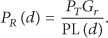
The free space radio propagation model is used to predict received signal strength when the transmitter and receiver have a clear, unobstructed line of sight path between them. This free space power received by a receiver antenna which is separated from a transmitter antenna by a distance d is given by the free space equation

$$\begin{array}{cc}& P_R\left(d\right)=\frac{P_T{G}_t{G}_r{\lambda }^{\mathrm{2}}}{\left({\mathrm{4}\pi }^{\mathrm{2}}\right)d^{\mathrm{2}}L},\end{array}$$

(1)

where $P_R(d)$ is the received power which is a function of d, $P_T$ is the transmitted power, d is the $\text{T-R}$ separation distance, $G_t$ is the transmitter antenna gain, $G_r$ is the receiver antenna gain, L is the path loss for a reference distance, and λ is the wavelength of the signal.

The signal propagation path loss for $\text{T-R}$ separation distance d is expressed as

$$\begin{array}{cc}& \text{Path}\mathrm{\hspace{0.17em}\hspace{0.17em}}\text{loss},\text{PL}\left(d\right)=\frac{\left({\mathrm{4}\pi }^{\mathrm{2}}\right)d^{\mathrm{2}}L}{{\lambda }^{\mathrm{2}}}.\end{array}$$

(2)

For Medical Implant Communication Services (MICS), the transmitting antenna is considered to be part of the channel [27]. For the MICS channel, the path loss includes the transmitter antenna gain:

$$\begin{array}{cc}& \text{PL}\left(d\right)=\frac{G_t\left({\mathrm{4}\pi }^{\mathrm{2}}\right)d^{\mathrm{2}}L}{{\lambda }^{\mathrm{2}}}.\end{array}$$

(3)

The received power can be expressed as

$$\begin{array}{cc}& P_R\left(d\right)=\frac{P_T{G}_r}{\text{PL}\left(d\right)}.\end{array}$$

(4)

The received signal strength in dBm can simply be expressed as follows:

$$\begin{array}{cc}& \text{RSSI}\left(\text{in}\mathrm{\hspace{0.17em}\hspace{0.17em}}\text{dBm}\right)=\left(G_r+P_T\right)\left(\text{in}\mathrm{\hspace{0.17em}\hspace{0.17em}}\text{dBm}\right)-\text{PL}\left(\text{in}\mathrm{\hspace{0.17em}\hspace{0.17em}}\text{dBm}\right).\end{array}$$

(5)

The most widely used path loss lognormal shadowing signal propagation model includes the path loss attenuations exponents which are different for different surroundings and varies due to the medium of propagation. The path loss in dB at some distance d can statistically be modeled by the following path loss lognormal shadowing equation:

$$\begin{array}{cc}& \text{PL}\left(d\right)=\text{PL}\left(d_0\right)+10\alpha {\log }_{\mathrm{10}}\frac{d}{d_0}+S.\end{array}$$

(6)

$d_0$ is the reference distance (where $d\ge d_0$ ) and α is the path loss exponent which heavily depends on the environment where RF signal is propagating through. For example, it is well-known that, for free space, $n=2$ . Human body is an extremely lossy environment; therefore, much higher value for the path loss exponent is expected. $S(0,{{\sigma }_{\text{RSS}}}^{\mathrm{2}})$ is the random scatter around the mean with standard deviation ${\sigma }_{\text{RSS}}$ in dB caused by different materials and antenna gain in different directions.

4. Proposed Localization Algorithm

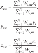
Weighted Centroid Localization (WCL) calculates the position of the target node using the sum of the weighted average of the reference nodes positions. WCL introduced the quantification of the nodes position depending on their distance to the target node. The aim is to give more influence to those nodes which are nearer to the target. The three-dimensional position of the target is calculated using WCL as follows:

$$\begin{array}{ll}& P_m\left(x_{\text{est}},y_{\text{est}},z_{\text{est}}\right)=\frac{{\sum }_{i=\mathrm{1}}^N{W}_{i,m}{B}_i\left(x,y,z\right)}{{\sum }_{i=\mathrm{1}}^N{W}_{i,m}}\\ =\frac{{\sum }_{i=\mathrm{1}}^N(\mathrm{1}/{\text{distance}}_{i,m})B_i\left(x,y,z\right)}{{\sum }_{i=\mathrm{1}}^N\left(\mathrm{1}/{\text{distance}}_{i,m}\right)},\end{array}$$

(7)

where $P_m(x_{\text{est}},y_{\text{est}},z_{\text{est}})$ is the estimated location for the mth position of the target. ${\text{distance}}_{i,m}$ denotes the distance of the ith reference node from the target's mth position. $B_i(x,y,z)$ is the known position of ith reference node; N is the number of reference nodes in the communication range (in our system $N=8$ ).

4.1. Linear Least Square-WCL (LLS-WCL): A VCE Localization Approach

In our proposed VCE localization approach, we have used WCL algorithm to calculate the three-dimensional position of the VCE using the corresponding weight of the reference nodes and their known positions. Figure 3 demonstrates our proposed approach of WCL to localize the VCE where the red object indicates the target VCE and the blue tags indicate the reference nodes. The VCE is equipped with a RF transmitter tag. As shown in Figure 3, a 3D receiver array of 8 RF receiver (Rx) nodes has been used to localize the mobile VCE at $(x,y,z)$ position. The dimension of the 3D array is 300 mm × 300 mm × 300 mm. The receivers are placed as the reference nodes at $(x_i,y_i,z_i)$ positions.

Figure 3

WCL algorithm.

$d_i$ indicates the distance of the receivers from the VCE which is used to calculate the weight of the sensors which is inversely proportional to the distance. In radio signal propagation, the received signal strength decreases as the distance of the $\text{Tx-Rx}$ increases as in (1). Therefore, we have used the radio propagation model to calculate the distance $d_i$ from the path loss $\text{PL}(d)$ using (6) where $\text{PL}(d)$ is calculated from the received signal strength RSSI using (5). In our proposed approach, the VCE transmits RF signal and the 8 receivers measure the signal strength (RSSI) of the received signal. The path loss $\text{PL}(d)$ is calculated from the RSSI which is an identifier of distance $d_i$ . Finally the weight of the sensors is calculated using (8) and the position of the VCE is calculated using WCL algorithm using (9). Consider

$$\begin{array}{cc}& W_{i,m}=\frac{\mathrm{1}}{\text{PL}\left(d_{i,m}\right)},\end{array}$$

(8)

where $W_{i,m}$ is the weight of the ith sensor for mth position of the VCE. Consider

$$\begin{array}{cc}& x_{\text{est}}=\frac{{\sum }_{i=1}^N{W}_{i,m}{x}_i}{{\sum }_{i=1}^N{W}_{i,m}},\\ y_{\text{est}}=\frac{{\sum }_{i=1}^N{W}_{i,m}{y}_i}{{\sum }_{i=1}^N{W}_{i,m}},\\ z_{\text{est}}=\frac{{\sum }_{i=1}^N{W}_{i,m}{z}_i}{{\sum }_{i=1}^N{W}_{i,m}}.\end{array}$$

(9)

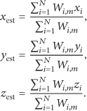
Figure 4 shows the simulation results using WCL for 2530 sample positions of the VCE where we can observe that there occurs a linear relationship between the estimated and real positions. We can express the relation of the estimated and real position by the following equation:

$$\begin{array}{cc}& {\mathrm{\hspace{0.17em}\hspace{0.17em}}P}_{A,m}\left(x,y,z\right)=C·P_{\text{est},m}\left(x_{\text{est}},y_{\text{est}},z_{\text{est}}\right),\end{array}$$

(10)

where $P_{A,m}$ and $P_{\text{est},m}$ are the real and estimated positions (coordinates) for m possible positions of the target. Using this linear relationship, a calibration process is applied using linear least square regression of the estimated and real locations to calculate the calibration coefficient, C. Finally C is used to calibrate the locations to find more accurate location of VCE which is indicated as the red line in Figure 4. We call this process of localization linear least square-WCL (LLS-WCL).

Figure 4

Position estimation and calibration using LLS-WCL.

A major challenge in this approach of VCE localization is that the weight calculated using uniform path loss cannot assure the same distance for different surroundings in the nonhomogeneous environment as human body. As we can see from (6) the path loss attenuation exponents ( $\text{PL}(d_0)$ , α and S) are important factors for distance calculation from the radio propagation model. Path loss attenuation exponents vary due to the environment and medium of propagation. Thus, to calculate the distance accurately, first we have to identify the path loss attenuation exponents for different surroundings where the target stays. The second issue in this regard is the random deviation of attenuation $S(0,{{\sigma }_{\text{RSS}}}^{\mathrm{2}})$ which is mainly caused due to the multipath and shadow fading effects. The path loss is scattered around a mean due to the deviations affecting the accuracy in weight calculation as well as the position estimation using WCL. As we can see in Figure 4, the estimated locations are scattered around a mean which is due to the random path loss deviations $S(0,{{\sigma }_{\text{RSS}}}^{\mathrm{2}})$ . Thus, the path loss deviations must be minimized to improve the localization accuracy.

4.2. Adaptive Linearized LLS-WCL: An Improved Method of VCE Localization

The adaptive linearized LLS-WCL includes the following steps of improvements.

(1) Statistical Path Loss Modeling. The statistics of the path loss model for specific surroundings is adaptively identified using linear least square regression of the experimentally collected data sets.

(2) Path Loss Linearization. This step is to minimize the path loss deviations by linearizing the path loss model considering minimum deviations.

(3) Weight Calculation and Position Estimation. In this step, the weight of the sensors is calculated from the linearized path loss and the position is estimated using WCL algorithm.

(4) Position Calibration. The final step is to identify the calibration coefficient (C) using the linear relationship of the estimated and real locations and then to calibrate the estimated positions using C to improve the localization accuracy.

The steps are briefly explained below.

4.2.1. Statistical Path Loss Modeling

We use the lognormal shadowing signal propagation model (as shown in (6)) to model the path loss for two different scenarios assuming ${{\sigma }_{\text{RSS}}}^{\mathrm{2}}$ deviations with 0 mean. Consider

$$\begin{array}{cc}& \text{PL}\left(d\right)=\text{PL}\left(d_0\right)+10\alpha {\log }_{\mathrm{10}}\frac{d}{d_0}+S\left(\mathrm{0},{{\sigma }_{\text{RSS}}}^{\mathrm{2}}\right).\end{array}$$

(11)

The path loss may be modelled using two different methods. The first method requires experimental data sets (path loss for variable $\text{Tx-Rx}$ separation distances) for different surroundings to find the statistics of the path loss model. However, no such reference data sets are currently available for medical implant communication service (MICS). The second method is simulation based [27] where the characteristics of radio propagation are analyzed using electromagnetic field simulator by setting different statistics of path loss model for different locations of the human body model. Such statistical data sets are available for MICS in [27].

Hence we follow the first method to model the path loss using our experimentally collected data sets (path loss versus distance) for two scenarios. We have also modelled the path loss using the statistics available in [27] for the MICS. The statistics ( $\text{PL}(d_0)$ , α and ${\sigma }_{\text{RSS}}$ ) of the path loss model can adaptively be identified for different scenario using linear least square regression of the entire data sets as follows.

We consider the signal propagation model of (11) as a linear system of equation in matrix form as follows:

$$\begin{array}{ll}& B=AX\\ \ge \left[\begin{array}{l}\text{PL}\left(d_{\mathrm{1}}\right)\\ \text{PL}\left(d_{\mathrm{2}}\right)\\ ⋮\\ \text{PL}\left(d_m\right)\end{array}\right]=\left[\begin{array}{lll}1& \mathrm{10}{\log }_{\mathrm{10}}\left(d_{\mathrm{1}}\right)& 1\\ 1& \mathrm{10}{\log }_{\mathrm{10}}\left(d_{\mathrm{2}}\right)& 1\\ ⋮& ⋮& ⋮\\ 1& \mathrm{10}{\log }_{\mathrm{10}}\left(d_m\right)& 1\end{array}\right]\left[\begin{array}{l}P\left(d_{\mathrm{0}}\right)\\ \alpha \\ {\sigma }_{\text{RSS}}\end{array}\right],\end{array}$$

(12)

where $\text{PL}(d)$ is the path loss calculated using (5) from the measured RSSI of the sensors for variable distances d for m several positions of the target. As B is only approximate due to the random deviations, the problem requires the determination of X such that $B\approx AX$ , where $B-AX$ is the residuals.

Minimizing the sum of the squares of the residuals leads to a normal equation as follows:

$$\begin{array}{cc}& A^{T}AX=A^{T}B,\\ X={\left(A^{T}A\right)}^{-\mathrm{1}}{A}^{T}B.\end{array}$$

(13)

Thus, we can calculate the path loss attenuation exponents ( $\text{PL}(d_0)$ , α and ${\sigma }_{\text{RSS}}$ ) for different scenario using the experimental data sets as follows:

$$\begin{array}{ll}& \left[\begin{array}{l}P\left(d_0\right)\\ \alpha \\ {\sigma }_{\text{RSS}}\end{array}\right]\\ \hspace{1em}={\left({\left[\begin{array}{lll}1& \mathrm{10}{\log }_{\mathrm{10}}\left(d_{\mathrm{1}}\right)& 1\\ 1& \mathrm{10}{\log }_{\mathrm{10}}\left(d_{\mathrm{2}}\right)& 1\\ ⋮& ⋮& ⋮\\ 1& \mathrm{10}{\log }_{\mathrm{10}}\left(d_m\right)& 1\end{array}\right]}^T\left[\begin{array}{lll}1& \mathrm{10}{\log }_{\mathrm{10}}\left(d_{\mathrm{1}}\right)& 1\\ 1& \mathrm{10}{\log }_{\mathrm{10}}\left(d_{\mathrm{2}}\right)& 1\\ ⋮& ⋮& ⋮\\ 1& \mathrm{10}{\log }_{\mathrm{10}}\left(d_m\right)& 1\end{array}\right]\right)}^{-\mathrm{1}}\\ \hspace{1em}\hspace{1em}·{\left[\begin{array}{lll}1& \mathrm{10}{\log }_{\mathrm{10}}\left(d_{\mathrm{1}}\right)& 1\\ 1& \mathrm{10}{\log }_{\mathrm{10}}\left(d_{\mathrm{2}}\right)& 1\\ ⋮& ⋮& ⋮\\ 1& \mathrm{10}{\log }_{\mathrm{10}}\left(d_m\right)& 1\end{array}\right]}^T\left[\begin{array}{l}\text{PL}\left(d_{\mathrm{1}}\right)\\ \text{PL}\left(d_{\mathrm{2}}\right)\\ ⋮\\ \text{PL}\left(d_m\right)\end{array}\right].\end{array}$$

(14)

4.2.2. Path Loss Linearization

Using the adaptively identified statistics ( $\text{PL}(d_0)$ , α and ${\sigma }_{\text{RSS}}$ ) of different scenario, the path loss is linearized to minimize the deviations. The linearized or mean path loss is obtained considering minimum deviations ( ${\sigma }_{\text{RSS}}=0$ ). After completion of this step the path loss is adaptively linearized. Consider

$$\begin{array}{cc}& \left[\begin{array}{c}{\text{PL}\left(d_1\right)}_{\mathrm{lin}}\\ {\text{PL}\left(d_2\right)}_{\mathrm{lin}}\\ ⋮\\ {\text{PL}\left(d_m\right)}_{\mathrm{lin}}\end{array}\right]=\left[\begin{array}{cc}1& \mathrm{10}{\log }_{\mathrm{10}}\left(d_1\right)\\ 1& \mathrm{10}{\log }_{\mathrm{10}}\left(d_2\right)\\ ⋮& ⋮\\ 1& \mathrm{10}{\log }_{\mathrm{10}}\left(d_m\right)\end{array}\right]\left[\begin{array}{c}\text{PL}\left(d_0\right)\\ \propto \end{array}\right],\end{array}$$

(15)

where ${\text{PL}\left(d_m\right)}_{\mathrm{lin}}$ is the linearized path loss for m possible positions of the target.

4.2.3. Weight Calculation and Position Estimation

The scattered path loss is attenuated to the adaptively linearized path loss and then used to calculate the weight of the sensors using (16). Consider

$$\begin{array}{cc}& W_{i,m}=\frac{\mathrm{1}}{{\text{PL}\left(d_{i,m}\right)}_{\mathrm{lin}}},\end{array}$$

(16)

where $W_{i,m}$ is the weight of the ith sensor for mth position of the target and ${\text{PL}(d_{i,m})}_{\mathrm{lin}}$ is the linearized path loss of the ith sensor for mth position of the target.

Using the weight of the sensors and their reference positions, the VCE is localized using WCL as follows using (17) where the weight is calculated using adaptively linearized path loss. Consider

$$\begin{array}{cc}& x_{\text{est}}=\frac{{\sum }_{i=\mathrm{1}}^N{W}_{i,m}{x}_i}{{\sum }_{i=\mathrm{1}}^N{W}_{i,m}},\\ y_{\text{est}}=\frac{{\sum }_{i=\mathrm{1}}^N{W}_{i,m}{y}_i}{{\sum }_{i=\mathrm{1}}^N{W}_{i,m}},\\ z_{\text{est}}=\frac{{\sum }_{i=\mathrm{1}}^N{W}_{i,m}{z}_i}{{\sum }_{i=\mathrm{1}}^N{W}_{i,m}}.\end{array}$$

(17)

4.2.4. Estimated Position Calibration

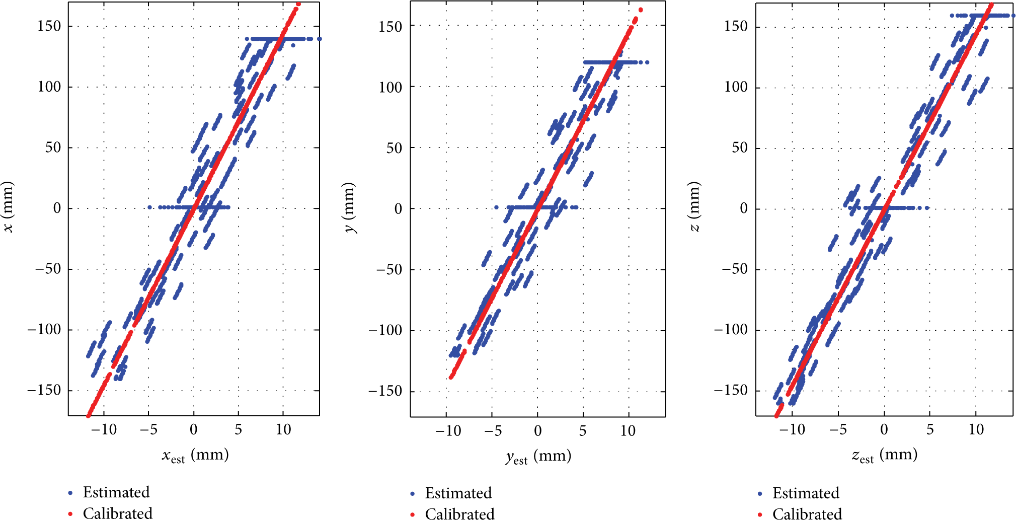
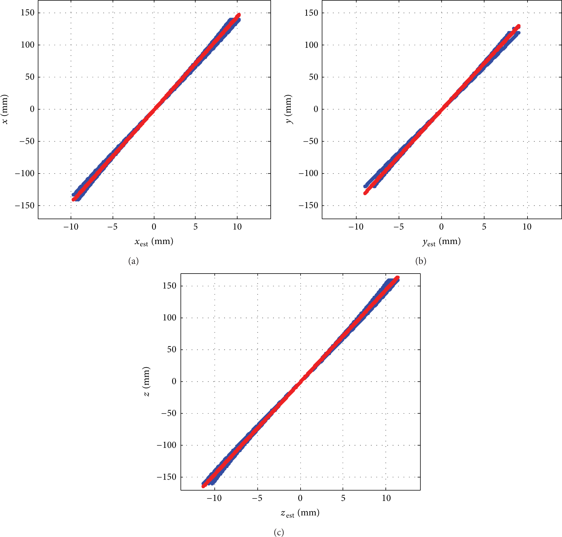
We can observe from the simulation results of adative linearized WCL that there is a linear relationship between the estimated and real positions as shown in Figure 5 which can be written as a linear system of equation as in (18). Consider

$$\begin{array}{cc}& {\mathrm{\hspace{0.17em}\hspace{0.17em}}P}_{A,m}\left(x,y,z\right)=C·P_{\text{est},m}\left(x_{\text{est}},y_{\text{est}},z_{\text{est}}\right).\end{array}$$

(18)

$P_{A,m}$ and $P_{\text{est},m}$ are all the actual and estimated coordinates in three dimensions for m possible positions of the target. Figure 5 shows the linear relationship of the real and estimated positions for 2,530 possible sample positions of the VCE. As we can see that, it is possible to calibrate the estimated positions using (19) to find a more accurate location of VCE if the calibration coefficient C is identified. Consider

$$\begin{array}{cc}& P_{C,m}\left(x,y,z\right)=C·P_{\text{est},m}\left(x_{\text{est}},y_{\text{est}},z_{\text{est}}\right),\end{array}$$

(19)

where $P_{C,m}\left(x,y,z\right)$ is the calibrated position for mth position.

Figure 5

Linear relationship between real and estimated position across x-y-z-axis (simulated 2,530 samples positions).

We can calculate C using linear least square regression of all estimated and real positions if (18) is considered as a linear system of equation in matrix form,

$$\begin{array}{cc}& P_A=P_E·C,\end{array}$$

(20)

where $P_A$ is the actual positions, $P_E$ is estimated positions, and C is the calibration coefficient.

As $P_A$ is approximate due to the standard deviations, the problem requires the determination of C such that $P_{E}C\approx P_A$ and $e=P_A-P_{E}C$ where e is the residuals. Minimizing the sum of the squares of the residuals leads to a normal equation

$$\begin{array}{cc}& \hspace{0.17em}{P_E}^T{P}_{E}C={P_E}^T{P}_A\hspace{1em}\text{or}\\ \hspace{0.17em}C={\left({P_E}^T{P}_E\right)}^{-\mathrm{1}}{P_E}^T{P}_A.\end{array}$$

(21)

Thus, the coefficient C is calculated using all the estimated and real positions using (22) and then a calibration process is applied using (23) to find more accurate location of the VCE using adaptive linearized LLS-WCL. Consider

$$\begin{array}{ll}& C={\left({\left[\begin{array}{lll}{x}_{\text{est}\mathrm{1}}& y_{\text{est}\mathrm{1}}& z_{\text{est}\mathrm{1}}\\ x_{\text{est}\mathrm{2}}& y_{\text{est}\mathrm{2}}& z_{\text{est}\mathrm{2}}\\ ⋮& ⋮& ⋮\\ x_{\text{est}m}& y_{\text{est}m}& z_{\text{est}m}\end{array}\right]}^T\left[\begin{array}{lll}{x}_{\text{est}\mathrm{1}}& y_{\text{est}\mathrm{1}}& z_{\text{est}\mathrm{1}}\\ x_{\text{est}\mathrm{2}}& y_{\text{est}\mathrm{2}}& z_{\text{est}\mathrm{2}}\\ ⋮& ⋮& ⋮\\ x_{\text{est}m}& y_{\text{est}m}& z_{\text{est}m}\end{array}\right]\right)}^{-\mathrm{1}}\\ \hspace{1em}·{\left[\begin{array}{lll}{x}_{\text{est}\mathrm{1}}& y_{\text{est}\mathrm{1}}& z_{\text{est}\mathrm{1}}\\ x_{\text{est}\mathrm{2}}& y_{\text{est}\mathrm{2}}& z_{\text{est}\mathrm{2}}\\ ⋮& ⋮& ⋮\\ x_{\text{est}m}& y_{\text{est}m}& z_{\text{est}m}\end{array}\right]}^T\left[\begin{array}{lll}{x}_{A1}& y_{A1}& z_{A1}\\ x_{A2}& y_{A2}& z_{A2}\\ ⋮& ⋮& ⋮\\ x_{Am}& y_{Am}& z_{Am}\end{array}\right],\end{array}$$

(22)

$$\begin{array}{ll}& \left[\begin{array}{lll}{x}_{c\mathrm{1}}& y_{c\mathrm{1}}& z_{c\mathrm{1}}\\ x_{c\mathrm{2}}& y_{c\mathrm{2}}& z_{c\mathrm{2}}\\ ⋮& ⋮& ⋮\\ x_{cm}& y_{cm}& z_{cm}\end{array}\right]=\left[\begin{array}{lll}{x}_{\text{est}\mathrm{1}}& y_{\text{est}\mathrm{1}}& z_{\text{est}\mathrm{1}}\\ x_{\text{est}\mathrm{2}}& y_{\text{est}\mathrm{2}}& z_{\text{est}\mathrm{2}}\\ ⋮& ⋮& ⋮\\ x_{\text{est}m}& y_{\text{est}m}& z_{\text{est}m}\end{array}\right]\left[C\right].\end{array}$$

(23)

5. Experimental Methodologies and System Development

The methodology is divided into the following steps.

5.1. Development of the Test System

The test system has been developed to collect data using two different scenarios. By weight, human body constitutes of 45%–65% water [32–34]. As air and water have completely different properties of radio propagation, we have chosen to perform the radio propagation test for Air to Air and for Air to Water interface scenarios to confirm that different scenarios have influence on the path loss.

The measurement setup for data collection using scenarios 1 and 2 has been shown in Figures 6 and 7. For scenario 1, both the transmitter and receiver have been placed in air. For scenario 2, the transmitter has been placed in air and the receiver has been placed inside the water. The test system may be divided into RF communication and data collection subsystems. The RF communication part is similar to the RF communication part in Figure 2. To develop the RF communication part, we have used 2.4 GHz ISM band Transceiver Module (RFM70) and ARM Coxtex-M4 microcontrollers. Tranceivers are used to transmit and receive radio signals; and the MCU has been used to configure the transceivers and to read-write data. The data collection part consists of the UART interface of MCU and the PuTTY terminal software of PC.

Figure 6

Scenario 1: measurement setup for data collection using Air to Air interface.

Figure 7

Scenario 2: measurement setup for data collection using Air to Water interface.

The radio signal transmitted by the transmitter is received by the receiver and the RSSI is measured. If the transmitter position is changed, the RSSI thresholds change accordingly. For both scenarios, we have collected the RSSI data for variable $\text{Tx-Rx}$ seperation distances. The UART interface of MCU and the PuTTY terminal has been used to collect RSSI data using the PC. We can send commands and read RSSI from the MCU using PuTTY. We can measure the $\text{Tx-Rx}$ separation distance using a centimeter-scaled rular.

5.2. Data Collection

We collect the measured RSSI of the receivers for variable $\text{TX-Rx}$ separation distances for two scenarios which have been presented in Table 1. Figure 8 shows the plot of the calculated path loss as a function of $\text{TX-RX}$ separation distance which has been plotted using Matlab. As we can see from the table and figure the path loss changes logarithmically as a function of distance and it is scattered around a mean. It can be explained using the shadow fading path loss model as in (11) where we can observe that the path loss is a linear function of the logarithm of distance and the path loss is scattered due to the random scattered deviation $S(0,{{\sigma }_{\text{RSS}}}^{\mathrm{2}})$ around a mean. The straight line through the scattered path loss is obtained using “least squares” method that best fits the collected data.

Table 1

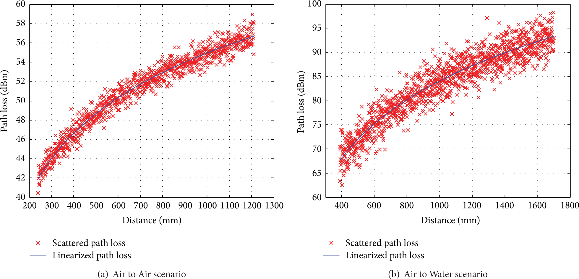
Path loss versus Tx-Rx separation distances [for selected points].

Air to Air scenario			Air to Water scenario
Distance (mm)	RSSI (dBm)	Path loss (dBm) PL(d) = $$G_R+P_T$$   − RSSI where $$G_R+P_T$$ = −25 dBm	Distance (mm)	RSSI (dBm)	Path loss (dBm)PL(d) = $$G_R+P_T$$   − RSSI where $$G_R+P_T$$ = 5 dBm
240	−67	42	500	−67	72
300	−69	44	640	−69	74
360	−71	46	900	−71	76
420	−73	48	1100	−75	80
600	−75	50	1260	−79	84
762	−77	52	1279	−81	86
912	−79	54	1300	−83	88
1062	−81	56	1500	−85	90
1211	−83	58	1680	−89	94

Figure 8

Distance based path loss model obtained from the measured data (path loss versus distance).

5.3. Path Loss Modelling

The statistics of the path loss have been extracted in Table 2 using linear least square regression of the measured data using (14).

Table 2

Extracted parameters using linear least square regression of the measured data.

Scenarios	Measurement parameters	PL( $$d_{\mathit{0}}$$ )	$$\alpha$$	S(0, $${{\sigma }_{\text{RSS}}}^{\mathrm{2}}$$ )
				Mean	$${\sigma }_{\text{RSS}}$$
Air to Air interface	Frequency band: 2.4 GHz Transmission power: −25 dBm Number of points: 980	42	2.08	0	0.74
Air to Water interface	Frequency band: 2.4 GHz Transmission power: 5 dBm Number of points: 1501	72	4.005	0	2.54

As we can see from the extracted statistics, the parameters are different for different scenarios which is due to the radio propagation property of different mediums. As the radio propagation property of air and water is different, much higher value of the path loss exponent and path loss deviations has been observed for the Air to Water scenario. Higher value of path loss exponent is observed due to the lossy characteristics of water. The path loss is also more scattered due to the shadow fading effects of the Air to Water scenario which is caused due to the nonhomogeneous medium of propagation.

As the radio propagation parameters are different for different mediums, we can model the path loss statistically using the extracted parameters. By considering the normal distribution of the path loss deviations $S(0,{{\sigma }_{\text{RSS}}}^{\mathrm{2}})$ , we model the path loss for both scenarios using the extracted parameters as shown in Figures 9(a) and 9(b).

Figure 9

Statistical model and path loss linearization.

Human body is a nonhomogeneous environment for radio propagation. Therefore, the path loss is not uniform. Thus, different values of the path loss attenuation exponents and deviations are expected for different scenarios. By adaptively identifying the statistics for different scenario or environment, we can model the path loss for different locations inside the human body. The extracted statistics for two different scenarios of MICS are available in [27] where a 3D visualization system for medical implants has been used to calculate the statistics of the path loss model. The main components of their simulation system include a three-dimensional virtual human body model, the propagation engine which is a three-dimensional full-wave electromagnetic field simulator (i.e., HFSS 1), the 3D immersive and visualization platform, and finally an implantable (or body surface) antenna. The 3D human body model includes frequency dependent dielectric properties of 300+ parts in a male human body which has a resolution of 2 mm. Table 3 summarizes the extracted parameters of their model. As we can see, the statistics are different for different scenarios and much higher values of the parameters are observed.

Table 3

Extracted parameters of the statistical implant path loss model for two different scenarios.

Implant to body surface	PL( $$d_{\mathit{0}}$$ )	$$\alpha$$	$${\sigma }_{\text{RSS}}$$
Deep-tissue	47.14	4.26	7.85
Near-surface	49.81	4.22	6.81

Small intestine is a deep-tissue organ and its standard size is 140 mm $\times$ 120 mm $\times$ 160 mm. Thus, we can model the path loss for small intestine by setting the statistics of deep-tissue organ. We have modelled the path loss for deep-tissue implant to body surface for 50–800 mm range of distance which has been plotted in Figure 10(a) considering normal distribution of deviations as shown in Figure 10(b).

Figure 10

(a) Path loss versus distance for deep tissue implant to body surface scenario. (b) Normal distribution of the path loss deviation due to shadow fading effects of deep tissue implant to body surface.

5.4. Path Loss Linearization and Weight Calculation

The path loss is linearized by finding the linear least squares regression line through the scattered path loss that best fits the collected data. In Figures 9(a), 9(b), and 10, the straight line through the scattered path loss indicates the linearized path loss for Air to Air, Air to Water, and the deep tissue implant scenarios. To analyze the performance of adaptively linearized WCL, we find the straight line by replacing the extracted value of $\text{PL}(d_0)$ and α in (15) considering minimum deviations of the points about the regression line. The results for few selected points are illustrated in Table 4.

Table 4

Path loss linearization using the statistics of the path loss.

Scattered path loss, PL(d) = $$P_T$$   − RSSImeasured				Linearized path loss, PL(d)linearized = PL( $$d_{\mathit{0}}$$ ) + $$\mathrm{10}\alpha {\log }_{\mathit{10}}d$$
= PL $$(d_{\mathit{0}})+\mathrm{10}\mathrm{\alpha }{\log }_{\mathrm{10}}\left(d/d_{\mathit{0}}\right)+S\mathrm{\hspace{0.17em}\hspace{0.17em}}(\mathrm{0},{{\mathrm{\sigma }}_{\text{RSS}}}^{\mathrm{2}})$$				(Considering minimum path loss deviations)
Air to Air		Air to Water		Air to Air		Air to Water
Distance (mm)	Path loss (dBm)	Distance (mm)	Path loss (dBm)	Distance (mm)	Path loss (dBm)	Distance (mm)	Path loss (dBm)
240	42	500	72	240	42	500	72
300	44	640	74	300	44.02445	640	76.29376
360	46	900	76	360	45.67855	900	82.22366
420	48	1100	80	420	47.07706	1100	85.71403
600	50	1260	84	600	50.31297	1260	88.07609
762	52	1279	86	762	52.48143	1279	88.33642
912	54	1300	88	912	54.11168	1300	88.61968
1062	56	1500	90	1062	55.49313	1500	91.10871
1211	58	1680	94	1211	56.68427	1680	93.07989

The weight of the sensors is calculated from the linearized path loss using (16). The relation of the weight factor (W) to the distance has been shown in Figure 11 where we can see that the weight decreases as a function of distance and it is not scattered as it has been calculated using linearized path loss where the deviations are minimized.

Figure 11

Weight versus distance for different scenarios.

5.5. Position Estimation and Calibration

Finally, the position of the target is calculated using WCL as shown in (17) and then calibrated using (23). We have used the calculated weights of the sensors and their reference positions to find the estimated position using WCL. As we can see in Figure 5 if we simulate the WCL algortithm to find the position of several points of small intestine in 1 mm resolution, then it is found that there is a linear relationship between the real and estimated positions. As there occurs a linear relationship, a calibration process may be applied where the calibration coefficient (C) is calcultaed using linear least square regression of the real and estimated positions using (22). The estimated position is then calibrated using (23) to find more accurate position. The calibration coefficient for different scenario has been summarized in Table 5. The results of position calibration have been shown in Figure 12 where the relationship of the real, estimated, and calibrated positions is presented. Thus, it is essential to extract the value of C for any specific scenario before localization. The blue scattered lines in the figure indicate the relation of the estimated position to the real positions whereas the red straight line indicates the calibrated location. We observe that the calibrated positions using adaptive linearized LLS-WCL are absolutely linear to the real position indicating the minimized location error.

Table 5

Calibration coefficient calculated using linear least square regression.

Scenarios	Calibration coefficient, C
Air to Air	16.17
Air to Water	12.38
Deep-tissue implant to body surface	14.55

Figure 12

Location estimation and calibration using adaptive linearized LLS-WCL and their relationships.

6. Simulation System

Due to practical limitations, as it is difficult to verify the accuracy of the proposed algorithm using a real human body, we have developed a simulation system using Matlab to verify the accuracy. The system includes a 3D virtual small intestine model, 8 receiver sensors, implanted transmitter, and the propagation engine. Figure 13 shows the overview of the 3D simulation system which includes the small intestine model of 140 mm $\times$ 120 mm $\times$ 160 mm dimension depicted by the spiral tunnel. The small intestine has been placed near to the center of the 3D receiver array so as to avoid the central effect of the centroid algorithm where the localization accuracy reduces from the center to outwards. The black dot indicates one of the sample positions of the capsule's transmitter which has been mapped using Matlab. We have mapped 2530 sample positions similarly while it travels through the small intestine model in 1 mm resolution. The blue tags indicate the receiver sensor's position. The sensor topology is such that the 8 sensors are placed at the edge points of a 300 mm $\times$ 300 mm $\times$ 300 mm dimension box. The transmitted signal of the implanted transmitter is received by each of receivers. The propagation of $\text{Tx-Rx}$ has been modelled by the extracted statistics of the path loss attenuation exponents ( $\text{PL}(d_0)$ , α and ${\sigma }_{\text{RSS}})$ of three different scenarios discussed earlier. The propagation engine includes the propagation models which calculate the RSSI of the receivers for each position of the capsule $\text{Tx}$ . Finally, the estimated position of the capsule is calculated using our proposed adaptive linearized LLS-WCL algorithm. We have simulated 2,530 sample positions to find the estimated position of the capsule using our developed simulation system. The results are shown in the folowing section.

Figure 13

Simulation system overview.

The overall system flow of the simulation system as discussed above has been shown in the block diagram in Figure 14.

Figure 14

System flow block diagram.

7. Simulation Results and Analysis

To verify the accuracy of localization, we have simulated 2530 sample positions (1 mm resolution) of the capsule to find the estimated position using our proposed adaptive linearized LLS-WCL algorithm. The simulation system has been developed using Matlab. The estimated positions of selected seven sample positions are shown in Figure 15.

Figure 15

Localization results using adaptive linearized LLS-WCL.

The localization accuracy can be verified using the performance indices as localization error (LE), root mean square error (RMSE), and the standard deviation of error (STD) which are calculated as follows. Localization error (LE) is defined as the difference between estimated and real position as follows:

$$\begin{array}{cc}& \text{Localization}\mathrm{\hspace{0.17em}\hspace{0.17em}}\text{Error},\hspace{0.17em}\text{LE}=\sqrt{{\left(P_{\text{est}}\left(x,y,z\right)-P_{\text{real}}(x,y,z)\right)}^2},\\ \text{LE}=\sqrt{{\left(x_{\text{est}}-x_{\text{real}}\right)}^{\mathrm{2}}+{\left(y_{\text{est}}-y_{\text{real}}\right)}^{\mathrm{2}}+{\left(z_{\text{est}}-z_{\text{real}}\right)}^{\mathrm{2}}}.\end{array}$$

(24)

$P_{\text{est}}\left(x,y,z\right)$ is the estimated position and $P_{\text{real}}\left(x,y,z\right)$ is the real position of the capsule. For N simulation results of N possible positions of the capsule, the root mean square error (RMSE) is

$$\begin{array}{cc}& \text{RMSE}=\frac{{\sum }_{i=\mathrm{1}}^N{\text{LE}}_i}{N}.\end{array}$$

(25)

The standard deviation of error is expressed as

$$\begin{array}{cc}& \text{Standard}\mathrm{\hspace{0.17em}\hspace{0.17em}}\text{Deviation},\hspace{0.17em}\text{STD}=\sqrt{\frac{{\sum }_{i=\mathrm{1}}^N{{(\text{LE}}_i-\text{RMSE})}^{\mathrm{2}}}{N}}.\end{array}$$

(26)

From Figure 14, it can be observed that the difference between the estimated and real position is very small. Table 6 summarizes the location estimation results for 2,530 simulated points and verifies the accuracy by finding the performance indices. As we can see from the results the root mean square error (RMSE) of localization is as low as 5.106 mm with standard deviation 3.5 mm.

Table 6

Adaptive linearized LLS-WCL simulation results.

Position	Estimated position after calibration, $$P_{c,m}$$ ( $$x,y,z$$ )	Real position, $$P_{A,m}$$ ( $$x,y,z$$ )	LE (mm)	RMSE (mm)All 2,530 positions	Standard deviation (mm)All 2,530 positions
1	(140, 115, 153)	(134, 107, 150)	10.19
2	(−137, 86.9, 80.5)	(−140, 84.2, 77.5)	5.05
3	(9.94, 71.5, 37.4)	(9.9, 72.9, 37.5)	1.40
4	(76.3, 122, −25.9)	(75.6, 126, −25)	4.06	5.15	3.5
5	(−132, 131, −95.4)	(−130, 128, −90)	6.13
6	(−7.25, 57.4, −134)	(−7, 56.4, −140)	6.55
7	(148, 130, −165)	(140, 120, −160)	13.92

We have also simulated the proposed algorithm using different scenarios and compared the results. Table 7 presents the results of different optimization stages and summarizes the accuracy improvement. It is observed that localization accuracy significantly improves using the adaptively linearized method of LLS-WCL algorithm. As we can see from the different stages of optimization in Table 7, the mean localization error (RMSE) is as high as 157.3 mm using RSSI based WCL algorithm without considering any optimization levels. If we estimate the position using scattered path loss based LLS-WCL using linear least square calibration where the deviations have not been minimized $({\mathit{\sigma }}_{\mathbf{R}\mathbf{S}\mathbf{S}}=7.85$ for deep tissue implant model), the RMSE is 113 mm with standard deviation 41 mm. It may be dropped to RMSE 22.6 mm considering the lower value of the path loss deviation as ${\mathit{\sigma }}_{\mathbf{R}\mathbf{S}\mathbf{S}}=1$ . If the path loss exponents are adaptively identified for different scenarios and the path loss model is linearized considering minimum path loss deviations, then it is possible to further improve the accuracy. In our proposed adaptive linearized LLS-WCL algorithm, we have applied all the four optimization levels and the accuracy has been significantly improved with the RMSE of 5.15 mm with standard deviation 3.5 mm. Figure 16 presents the comparison of the localization results for all 2,530 sample target positions using WCL, LLS-WCL, and adaptively linearized LLS-WCL where S indicates the path loss deviation ${\sigma }_{\text{RSS}}$ . It can be observed that, using adaptive linearized LLS-WCL, much better accuracy in VCE localization has been obtained. It is also observed in Figure 15 that the accuracy depends on the path loss deviations (S) for which the LE increases. In our proposed algorithm, the accuracy has been significantly improved by minimizing the deviations using path loss linearization.

Table 7

Different stage of optimization and performance comparison of the adaptively linearized LLS-WCL algorithm.

Algorithms	Weight	Optimization stages		Experiment scenario	Path loss exponent, $$\alpha$$	Path loss deviation $${\sigma }_{\text{RSS}}$$	RMSE (mm)	STD (mm)
		Linear regression path loss modelling	Position calibration using linear regression
WCL	Scattered RSSI	No	No	Deep-tissue implant	4.26	7.85	157.3	69.09
WCL	Scattered path loss	No	No	Air to Air	2.08	0.74	139.6	61.6
				Air to Water	4.005	2.54	137.02	60.04
				Deep tissue implant	4.26	7.85	139.4	60.6
Adaptively linearized WCL	Linearized path loss	Yes	No	Air to Air	2.08	0.74	139.6	61.6
				Air to Water	4.005	2.54	136.8	60.32
				deep tissue implant	4.26	7.85	138.6	61.14
LLS-WCL	Scattered path loss	No	Yes	Air to Air	2.08	0.74	40.3	16.6
				Air to Water	4.005	2.54	64.46	27.26
				deep tissue implant	4.26	7.85	113.8	41
Adaptively linearized LLS-WCL	Linearized path loss	Yes	Yes	Air to Air	2.08	0.74	4.9	3.38
				Air to Water	4.005	2.54	5.58	3.7
				deep-tissue implant	4.26	7.85	5.15	3.5

Figure 16

Comparison of the localization accuracy of adaptive linearized LLS-WCL in different stage of optimizations (plotted using the simulated results for 2530 sample target positions in 1 mm resolution).

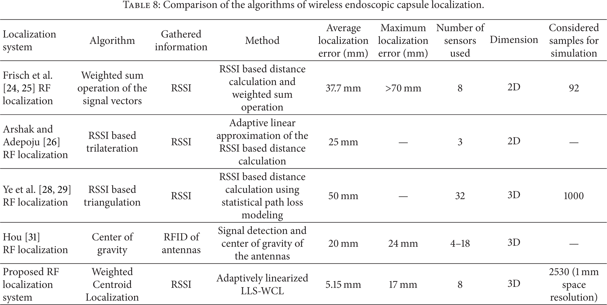
Table 8 compares our path loss based LLS-WCL approach with other previously proposed approaches. The authors in [24] proposed a 2D RF localization system using RSSI based triangulation method where 8 sensors were used to measure signal strengths which was later used to estimate the distance. The average experimental error was reported to be 37.7 mm [25] using a maximum of 92 samples. In [26], the authors proposed an adaptive linearized method of 2D localization of the moving telemetry capsule using RSS based triangulation method. They reported an average error of about 25% using 3 sensors. Based on the statistical implant path loss model developed in [27], the authors in [28, 29] used RSS based triangulation technique to analyze possible capsule localization accuracy in 3D location estimation using maximum 1000 samples and reported average localization error of 50 mm in all organs where more than 32 sensors on body surface are needed for achieving satisfactory localization accuracy. In [31], the authors present a localization system based on UHF band RFID. They propose a location estimation algorithm by calculating center of gravity of antennas which have detected the tag, and the results show a mean localization error of 2 cm. Using our proposed adaptively linearized method of path loss based WCL, average localization error of 5.106 mm is achievable in 3D position estimation in 1 mm spatial resolution (2,530 samples) using only 8 sensors. After comparing the results, it can be said that the proposed algorithm significantly improves the localization accuracy in 3D location estimation using only eight sensors with higher space resolution.

Table 8

Comparison of the algorithms of wireless endoscopic capsule localization.

Localization system	Algorithm	Gathered information	Method	Average localization error (mm)	Maximum localization error (mm)	Number of sensors used	Dimension	Considered samples for simulation
Frisch et al. [24, 25] RF localization	Weighted sum operation of the signal vectors	RSSI	RSSI based distance calculation and weighted sum operation	37.7 mm	>70 mm	8	2D	92
Arshak and Adepoju [26] RF localization	RSSI based trilateration	RSSI	Adaptive linear approximation of the RSSI based distance calculation	25 mm	—	3	2D	—
Ye et al. [28, 29] RF localization	RSSI based triangulation	RSSI	RSSI based distance calculation using statistical path loss modeling	50 mm	—	32	3D	1000
Hou [31] RF localization	Center of gravity	RFID of antennas	Signal detection and center of gravity of the antennas	20 mm	24 mm	4–18	3D	—
Proposed RF localization system	Weighted Centroid Localization	RSSI	Adaptively linearized LLS-WCL	5.15 mm	17 mm	8	3D	2530 (1 mm space resolution)

8. Conclusion

Path loss based WCL is a simple localization algorithm to determine the three-dimensional location of the wireless capsule endoscope inside the small intestine. A major challenge in this approach is the path loss attenuation exponents and the shadow fading effects which is caused due to the nonhomogeneous environment for radio propagation inside the human body resulting in certain level of path loss deviations S and different value of path loss attenuation exponents for different surroundings. The localization accuracy using path loss based WCL heavily depends on the path loss attenuation exponents and the path loss deviations. As we observed the mean localization error increases by 8-9 mm for each 1 dBm path loss deviation. In this paper, we propose an adaptive linearized method of WCL algorithm for VCE localization which includes four steps of optimizations to improve the localization accuracy. First we identify the path loss attenuation exponents or path loss statistics for different scenarios/surroundings using linear least square regression of the collected data set. Then we linearize the path loss model to minimize path loss deviations. Then we calculate the weights of the sensors using the linearized path loss and then estimate the VCE location using adaptively linearized WCL. Finally we calibrate the location using linear least square regression. We simulate our proposed adaptively linearized LLS-WCL algorithm using Matlab for 2530 possible sample positions inside the small intestine. The simulation results show significant accuracy improvement in 3D localization of the VCE inside the small intestine with root mean square error of 5.15 mm with standard deviation 3.5 mm using only 8 RF receiver sensors.