A New Approach for Coverage Analysis of Multihop Cooperative Networks Subject to Lognormal-Rice Fading

Abstract

A strip-shaped sensor network is considered, where randomly placed nodes communicate cooperatively by forming an opportunistic large array (OLA). The transmission from a group of cooperating nodes to another group of nodes is modeled with a quasi-stationary Markov chain, where the transmission channel is assumed to experience lognormal shadowing and Rice fading. The distribution of received power at a node is calculated as a three-step process, which includes finding the distribution of random distance between nodes in addition to other channel impairments, that is, fading and shadowing. It is shown that, in the presence of all three channel impairments, the received power at a node follows a lognormal distribution. This approximation uses a series of steps that involves techniques such as moment matching and moment generating function (MGF). Using the underlying Markov chain properties, the one-hop success probability of the network is derived. The system performance and coverage range of the network are quantified as a function of various network parameters and node topologies. The theoretical results are validated by performing computer simulations.

1. Introduction

Ever growing increase for efficient and reliable data delivery in future wireless systems suggests the use of cooperative transmission (CT). CT suppresses the issues of high latency and low reliability by employing distributed single-antenna nodes that receive multiple copies of the same message signal, thereby providing spatial diversity. The spatial diversity improves the received signal-to-noise ratio (SNR) by limiting the effects of multipath fading and shadowing present in a wireless channel. A dense wireless sensor network (WSN), following a multihop arrangement, widely uses CT for communication. The deployment of sensor networks can be used where low-power and low-cost data accumulation is required, such as monitoring and controlling indoor temperature or broadcasting of abnormal traffic events. Opportunistic large arrays (OLAs) are one of the most effective CT techniques used at the physical layer, where the nodes in a multihop network form groups, and these groups communicate with each other cooperatively [1]. Transmission takes place in presynchronized time slots because each group is assumed to have prior preamble synchronization for symbol and time coordination and easy channel access [2, 3]. All nodes in a group receive the same message signal and the receiving nodes decode the message using a diversity scheme and become part of the transmitting nodes towards next group. In densely populated networks, OLA provides a promising feature of long distance broadcasting with less power consumption [4].

Many works have been done in practical implementation of CT such as [5–7]. Similarly, numerous authors have exploited various properties of OLA. In [8], Mergen and Scaglione used continuum approximation approach, that is, fixed amount of transmit power per unit area along with infinite density of nodes. Although their model ensures end-to-end delivery, the study provided asymptotic results for very large density of nodes. On the other hand, there is generally a finite node density in wireless networks and infinite propagations are prohibited. For finite number of nodes, a linear network model is proposed in [9]. The analytical model depicts the successful finite number of hop counts before the transmission fails for a fixed distance between nodes. A 2-dimensional strip network is considered in [10], where authors studied the energy efficiency of an OLA strip network. Transmission protocols involving OLA, such as OLAROAD [11] and OLACRA [12], define cooperative route spans constructed over strip-shaped multihop networks.

In literature, a considerable amount of studies can be found on OLA networks under the impact of multipath fading; however, only Rayleigh fading model is widely used along with path loss [13–16]. This assumption may be used for simple network analysis; however, to gain practical insights into the network coverage, all major factors that impair wireless propagation should be considered. Generally, we characterize the fading phenomenon to be small-scale or large-scale. A practical channel model for small-scale fading in WSNs is Rice fading model as the possibility of line-of-sight (LOS) component increases during the deployment of sensor nodes [17]. Also the Rice fading is a more generalized form of fading that can be specialized to Rayleigh fading by changing its parameters. Similarly, a widely used model for large-scale fading (or shadowing) obeys the lognormal distribution [18, 19]. A cooperative network with Suzuki fading was studied in [20]; however, a linear topology was considered. To further extend the work, in this paper, we propose a geometric model for a 2-dimensional (2D) strip-shaped OLA network where each node broadcasts the message by using decode-and-forward (DF) technique, whereas the wireless channel undergoes lognormal shadowing and Rice fading. Our 2-dimensional network comprises hypothetical adjacent square regions with each region comprising of known number of randomly placed nodes. It is different from a typical OLA network in which irregular boundaries are formed by a group of nodes that increase the geometric complexity. The reason for this formation of 2-dimensional strip-shaped network is that the nodes of two neighboring regions form a disjoint set [21]. The fixed boundary confines the transmission from nodes only to the adjacent region.

We model the process of transmission between a set of nodes transmitting the same message signal to another set as a discrete-time Markov chain. At any level, the success probabilities of all the nodes are equal to one another. At a particular node, the received signal is a sum of multiple transmitted signals received over orthogonal channels [22]. We assume that the transmit power of all the nodes is the same and correct decoding occurs when a node's received power after postdetection combining is greater than a defined threshold.

Our contributions include the derivation of the probability density function (PDF) of SNR at a node, which is a stochastic process that includes a ratio distribution of a lognormal random variable (RV) and random distance RV, along with Rice fading. The effect on network's coverage area is quantified as a function of path loss exponent, Rice K-factor, and standard deviation of shadowing.

The rest of the paper is organized as follows. Section 2 describes the system model. In Section 3, we define our network's propagation model as a discrete-time Markov chain. We derive the transition probability matrix of the Markov chain in Section 4. Section 5 shows results of our analytical models and Section 6 concludes the paper along with future work.

2. System Model

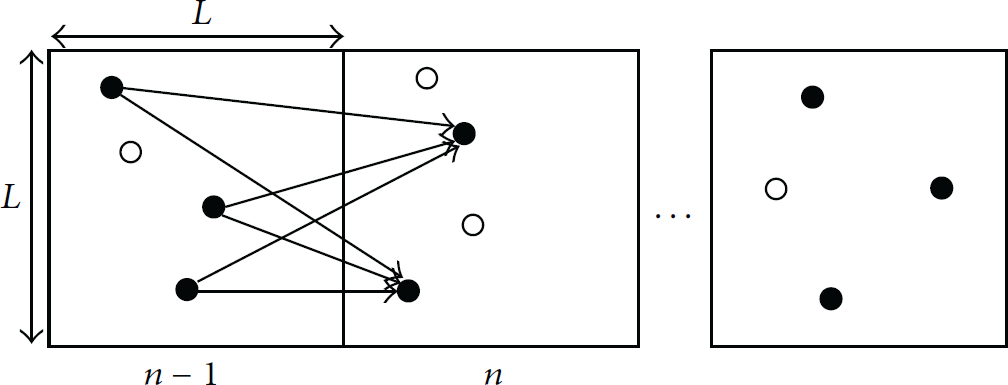
In this section, we describe the network layout and present an expression to compute the received power. An extended strip-shaped network is considered where each hop or level is a square region of area $\mathbb{A}$ such that $\mathbb{A}=L\times L$ . Each level contains N randomly placed nodes as shown in Figure 1. Let Γ denote the point process on the bounded set $\mathbb{A}$ , $\mathbb{A}\in {\mathfrak{R}}^{\mathrm{2}}$ , where $\Gamma (\mathbb{A})=N$ with probability 1, such that the placement of nodes in $\mathbb{A}$ is random with a uniform distribution. The wireless propagations are considered to be impacted by three channel impairments: path loss between randomly distributed nodes, large-scale shadowing, and small-scale fading.

Figure 1

Illustration of geometric strip-shaped network for $N=\mathrm{4}$ .

At each level, the N nodes form an OLA, cooperating synchronously to transmit the same message to the nodes in the next level using a decode-and-forward (DF) method. However, for a node to successfully decode the message signal, the received signal-to-noise ratio (SNR) should be greater than or equal to a defined decoding threshold, τ. As illustrated in Figure 1, the nodes that are not able to decode the message signal are shown to be hollow whereas the nodes filled in black are the ones that decoded the message signal correctly.

Assuming each node transmits with power $P_t$ , the received power, $P_{r_m}$ , at any node m at a level n in the network can be represented by

$$\begin{array}{cc}& P_{r_m}\left(n\right)={\displaystyle \sum }_{k\in {\mathcal{M}}_{n-\mathrm{1}}}\frac{P_t{\left(\nu q\right)}_{mk}}{{\left(d_{mk}\right)}^{\beta }},\end{array}$$

(1)

where $d_{mk}$ is the Euclidean distance between the node k at level $n-\mathrm{1}$ and node m at level n and β is the path loss exponent, whereas ${\nu }_{mk}$ represents a small-scale RV (Rice fading) and $q_{mk}$ is a large-scale lognormal RV between a node k at level $n-\mathrm{1}$ and a node m at level n with mean, μ, and variance, ${\sigma }^{\mathrm{2}}$ . In (1), the summation is over a set ${\mathcal{M}}_{n-\mathrm{1}}$ , where ${\mathcal{M}}_{n-\mathrm{1}}$ is the set of DF nodes at level $n-\mathrm{1}$ . The cardinality of the set ${\mathcal{M}}_{n-\mathrm{1}}$ is always less than or equal to N; that is, $\left|{\mathcal{M}}_{n-\mathrm{1}}\right|\le N$ .

3. Propagation Model

In this section, we model the hop-transmissions in the network by using Markov chains. Successful transmissions are assumed if a node's received power is greater than or equal to a defined decoding threshold, τ. We define ${\mathbb{I}}_j(n)$ as a binary RV reflecting the state of jth node at level n. This implies that a node can be in either state $\mathrm{1}$ , if it decodes the data properly, or state $\mathrm{0}$ if it does not decode the data. At a particular level containing N nodes, the binary indicator functions of all the nodes can be combined to constitute a single state, which represents the state of the system for that level. For example, at a level n, if $N=4$ and only one node has decoded the data, then possible system states could be $[\mathrm{1000}],[\mathrm{0100}],[\mathrm{0010}],[\mathrm{0001}]$ . This is because the nodes are randomly placed and not tagged. Therefore, we denote the state of a particular hop n based upon the number of DF nodes in a level; that is, $\mathcal{Y}(n)={\sum }_{j=\mathrm{1}}^N‍{\mathbb{I}}_j(n)$ . Furthermore, notice that node participation depends on the condition that at least one node at level $n-\mathrm{1}$ has transmitted; hence $\mathcal{Y}(n)$ depends only on $\mathcal{Y}(n-\mathrm{1})$ making $\mathcal{Y}$ a finite state Markov chain. Moreover, there can be a possibility where no node in a level decodes the message, the point where Markov chain enters the absorbing state, $\{\mathrm{0}\}$ , resulting in no further propagations. Thus $\mathcal{Y}(n)$ can be defined as a homogeneous finite state Markov chain, defined on two sets; that is, $\mathcal{Y}(n)\in \left\{\mathrm{0}\right\}\cup \mathbf{S}$ , where S is the irreducible state space given as

$$\begin{array}{cc}& \mathbf{S}=\left\{\begin{array}{cc}\mathrm{1}\hfill & \text{Precisely\hspace{0.17em}\hspace{0.17em}one\hspace{0.17em}\hspace{0.17em}node\hspace{0.17em}\hspace{0.17em}<!--?brm?-->decodes<!--?erm?-->}\hfill \\ \mathrm{2}\hfill & \text{Precisely\hspace{0.17em}\hspace{0.17em}two\hspace{0.17em}\hspace{0.17em}nodes\hspace{0.17em}\hspace{0.17em}<!--?brm?-->decode<!--?erm?-->}\hfill \\ ⋮\hfill & \hfill \\ N\hfill & \text{Precisely\hspace{0.17em}\hspace{0.17em}all\hspace{0.17em}\hspace{0.17em}nodes\hspace{0.17em}\hspace{0.17em}<!--?brm?-->decode.<!--?erm?-->}\hfill \end{array}\right.\end{array}$$

(2)

We also assume that the channel statistics remain the same and synchronous transmission occurs at every distinct time slot with each node having equal transmit power. This Markov chain can be defined by an $(N+\mathrm{1})\times (N+\mathrm{1})$ -dimensional transition probability matrix, $\tilde{\mathbf{T}}$ . However, we are only interested in finding the state of the system just before the transmission stops. By removing the first column and first row of the matrix, transitions to and from absorbing state reduce $\tilde{\mathbf{T}}$ to $N\times N$ dimension, forming a new submatrix, T, which is an irreducible square matrix with nonnegative entries and state space S. According to Perron-Frobenius theorem [23], there exist a unique maximum eigenvalue, ρ, and a unique eigenvector, v, for the matrix T such that $\mathbf{v}\mathbf{T}=\rho \mathbf{v}$ . The elimination of state 0 makes T a right substochastic matrix; that is, the value of Perron eigenvalue will always be less than unity. The state distribution of the system before going into killing (absorbing) state is called the quasi-stationary distribution; if v is the left eigenvector of matrix, T, then $\mathbf{v}=(v_i,i\in \mathbf{S})$ is the ρ-invariant distribution. Hence quasi-stationary distribution for the Markov chain at any state i becomes

$$\begin{array}{cc}& \mathbb{P}\left\{\mathcal{Y}\left(n\right)=i\hspace{0.17em}|\hspace{0.17em}\mathcal{K}>n\right\}=v_i,\hspace{1em}i\in \mathbf{S},\hspace{0.17em}\hspace{0.17em}\forall n,\end{array}$$

(3)

where $\mathcal{K}=\mathrm{i}\mathrm{n}\mathrm{f}\{n\ge \mathrm{0}:\mathcal{Y}(n)=\mathrm{0}\}$ is the event of absorbing state. The probability of being in state, i, at a certain level n, can be calculated as

$$\begin{array}{cc}& \mathbb{P}\left\{\mathcal{Y}\left(n\right)=i\right\}={\rho }^n{v}_i,\hspace{1em}i\in \mathbf{S},\hspace{0.17em}\hspace{0.17em}n\ge \mathrm{0}.\end{array}$$

(4)

4. Formulation of the Transition Matrix

At one hop, a node receives multiple copies of the same message signal under the impacts of multipath fading, shadowing, and path loss. The received SNR at the ith node at level n is given by ${\gamma }_i(n)=P_{r_i}(n)/{\sigma }_N^{\mathrm{2}}$ , where $P_{r_i}$ is the received power as given in (1) and ${\sigma }_N^{\mathrm{2}}$ is the variance of white noise. For node i to successfully decode a message signal at level n,

$$\begin{array}{cc}& P_s=\mathbb{P}\left\{\text{Success\hspace{0.17em}\hspace{0.17em}of\hspace{0.17em}\hspace{0.17em}node\hspace{0.17em}\hspace{0.17em}}i\hspace{0.17em}|\hspace{0.17em}\epsilon \right\}=\mathbb{P}\left\{{\mathbb{I}}_i\left(n\right)=\mathrm{1}\hspace{0.17em}|\hspace{0.17em}\epsilon \right\}=\mathbb{P}\left\{{\gamma }_i\left(n\right)>\tau \hspace{0.17em}|\hspace{0.17em}\epsilon \right\}={{\displaystyle \int }}_{\tau }^{\infty }{p}_{{\gamma }_i\hspace{0.17em}|\hspace{0.17em}\epsilon }\left(z\right)\mathrm{d}z,\end{array}$$

(5)

where $p_{{\gamma }_i\hspace{0.17em}|\hspace{0.17em}\epsilon }(z)$ is the conditional PDF of the received SNR, conditioned on the previous state $\epsilon \in \mathbf{S}$ . From (5), we can define the outage probability as $P_o=\mathrm{1}-P_s$ .

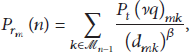
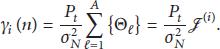
To compute the state transition probabilities, we need to find the success probability of each node in a certain level, n, given that $\left|{\mathcal{M}}_{n-\mathrm{1}}\right|$ nodes transmitted in the previous level, which can be computed via (5). Notice that, for a certain number of transmitting nodes, that is, $\left|{\mathcal{M}}_{n-\mathrm{1}}\right|$ , and constant network conditions, that is, transmit power, $P_t$ , path loss exponent, β, and region length L, the success probability for all N nodes at a particular level n will be the same. This is because the received power in (1) is RV where the distance between the nodes and the fading gains are both random. Therefore, if $s_{\mathrm{1}}$ and $s_{\mathrm{2}}$ are the states of the system, then the conditional probability of transition from state $s_{\mathrm{1}}$ to another state $s_{\mathrm{2}}$ , for $s_{\mathrm{1}},s_{\mathrm{2}}\in \mathbf{S}$ , can be found by using the binomial theorem; that is,

$$\begin{array}{cc}& \mathbb{P}\left(s_{\mathrm{1}}\hspace{0.17em}|\hspace{0.17em}{s}_{\mathrm{2}}\right)=\left(\begin{array}{c}N\\ s_{\mathrm{2}}\end{array}\right)P_s^{s_{\mathrm{2}}}{\left(P_o\right)}^{N-s_{\mathrm{2}}},\end{array}$$

(6)

where $P_s$ is as defined in (5). Notice that, in (6), the contribution of state $s_1$ has already been accounted for in the calculation of $P_s$ (or $P_o$ ) using (5), as the calculation of $P_s$ involves the knowledge of DF nodes at the previous level. We now proceed to find the outage (or success) probability of a single node at an arbitrary state. From (1), we can see that the received power at a node is a stochastic process that includes three RVs, namely, random distance, shadowing, and fading. If we define Θ to be RV that encompasses all these effects, then Θ can be given as

$$\begin{array}{cc}& \Theta =\frac{XR}{W}.\end{array}$$

(7)

Here we are considering a single-input single-output (SISO) link between a DF node of previous level and a single node of the current level. Once the calculation for SISO links is performed, we can then generalize it to a multiple-input single-output (MISO) link to calculate $P_s$ in (5). The RV X in (7) defines lognormal shadowing on the link, R denotes the multipath fading, and the RV W is used to denote the Euclidean distance between two nodes. It is shown in [24] that the random distance between a pair of nodes, when nodes are placed in adjacent square region, can be approximated by a Weibull RV. The distribution of the Euclidean distance raised to any power β is given by

$$\begin{array}{cc}& p_W\left(w\right)\approxeq \frac{c}{{\chi }^c}{w}^{c-\mathrm{1}}{\mathrm{e}\mathrm{x}\mathrm{p}}^{-{\left(w/\chi \right)}^c},\end{array}$$

(8)

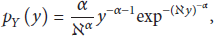
where $c=\mathrm{2}p/\beta$ is the shape parameter and $\chi ={\lambda }^p$ , for $\lambda =\mathrm{4}{L}^{\mathrm{2}}/(\mathrm{3}\Gamma (\mathrm{1.6327}))$ , is the scale parameter of Weibull distribution with constant $p=\mathrm{1.5806}$ . Here L is the length of the square region. The following sequence of work is now used to find the PDF of RV defined by (7). At first we compute the PDF of the ratio of lognormal RV, X, and Weibull RV, W, using the product distribution between lognormal and inverse Weibull distribution. We then compute another product distribution to find the PDF of RV in (7).

Let $W~\mathrm{W}\mathrm{e}\mathrm{i}\mathrm{b}\mathrm{u}\mathrm{l}\mathrm{l}(c,\chi )$ ; then $Y=\mathrm{1}/W$ is the $\mathrm{I}\mathrm{n}\mathrm{v}\mathrm{W}\mathrm{e}\mathrm{i}\mathrm{b}\mathrm{u}\mathrm{l}\mathrm{l}(\alpha ,\aleph )$ , where the inverse Weibull distribution is given by

$$\begin{array}{cc}& p_Y\left(y\right)=\frac{\alpha }{{\aleph }^{\alpha }}{y}^{-\alpha -\mathrm{1}}{\mathrm{e}\mathrm{x}\mathrm{p}}^{-{\left(\aleph y\right)}^{-\alpha }},\end{array}$$

(9)

where the scale and shape parameters are the same as that of Weibull distribution. We now find the product distribution of lognormal and inverse Weibull RVs using the following lemma.

Lemma 1.

The product of an inverse Weibull RV, Y, and a lognormal RV, X, can be approximated by another lognormal RV, Z, with mean ${\mu }_Z=\left(\mathrm{1}/\zeta \right)(C/\alpha -\mathrm{l}\mathrm{n}\aleph )+{\mu }_X(dB)$ and variance ${\sigma }_Z^{\mathrm{2}}={\pi }^{\mathrm{2}}/\mathrm{6}{\zeta }^{\mathrm{2}}{\alpha }^{\mathrm{2}}+{\sigma }_X^{\mathrm{2}}$ , where $C=\mathrm{0.5772}$ and $\zeta =\mathrm{l}\mathrm{n}(\mathrm{10})/\mathrm{10}$ , ${\mu }_X$ and ${\sigma }_X^{\mathrm{2}}$ are the mean and variance of X, and α and ℵ are the scale and shape parameters of Y.

Proof.

The distribution of a product RV $Z=XY$ is generally given by

$$\begin{array}{cc}& p_Z\left(z\right)={{\displaystyle \int }}_{-\infty }^{\infty }\frac{\mathrm{1}}{\left|x\right|}{f}_X\left(x\right)f_Y\left(\frac{z}{x}\right)\mathrm{d}x.\end{array}$$

(10)

The PDF of the product of lognormal and inverse Weibull RV can thus be expressed by the following equation:

$$\begin{array}{cc}& p_Z\left(z\right)=\frac{\alpha }{\zeta {\aleph }^{\alpha }{\sigma }_X\sqrt{\mathrm{2}\pi }}{{\displaystyle \int }}_{\mathrm{0}}^{\infty }\frac{\mathrm{1}}{x^{\mathrm{2}}}{\left(\frac{x}{z}\right)}^{\alpha +\mathrm{1}}\mathrm{e}\mathrm{x}\mathrm{p}\left\{-{\left(\frac{x\aleph }{z}\right)}^{\alpha }\right\}·\mathrm{e}\mathrm{x}\mathrm{p}\left\{\frac{-{\left(\mathrm{10}\hspace{0.17em}{\log }_{\mathrm{10}}\left(x\right)-{\mu }_{X_{\left(\mathrm{d}\mathrm{B}\right)}}\right)}^{\mathrm{2}}}{\mathrm{2}{\sigma }_{X_{\left(\mathrm{d}\mathrm{B}\right)}}^{\mathrm{2}}}\right\}\mathrm{d}x.\end{array}$$

(11)

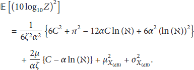
It can be noticed that the product distribution does not exist in a closed-form. Hence we use the moment matching technique to calculate the moments of approximating lognormal RV, $Z=\mathrm{1}{\mathrm{0}}^{\varphi /\mathrm{10}}$ such that $\varphi ~\mathcal{N}({\mu }_{\varphi },{\sigma }_{\varphi }^{\mathrm{2}})$ and $Z~\mathrm{l}\mathrm{o}\mathrm{g}\mathcal{N}({\mu }_{\varphi },{\sigma }_{\varphi }^{\mathrm{2}})$ . Since Z is lognormal, therefore, the computation of the first two moments is sufficient. To extract the mean and variance from (11) consider finding the first moment of the associated normal RV; that is,

$$\begin{array}{cc}& {\mu }_{\varphi }=\mathbb{E}\left[\mathrm{10}\hspace{0.17em}{\log }_{\mathrm{10}}Z\right]=\frac{\alpha }{\zeta {\aleph }^{\alpha }{\sigma }_X\sqrt{\mathrm{2}\pi }}{{\displaystyle \int }}_{\mathrm{0}}^{\infty }\mathrm{10}\hspace{0.17em}{\log }_{\mathrm{10}}\left(z\right)·{{\displaystyle \int }}_{\mathrm{0}}^{\infty }\exp \left\{-{\left(\frac{x\aleph }{z}\right)}^{\alpha }\right\}\mathrm{e}\mathrm{x}\mathrm{p}\left\{\frac{-{\left(\mathrm{10}\hspace{0.17em}{\mathrm{l}\mathrm{o}\mathrm{g}}_{\mathrm{10}}\left(x\right)-{\mu }_{X_{\left(\mathrm{d}\mathrm{B}\right)}}\right)}^{\mathrm{2}}}{\mathrm{2}{\sigma }_X^{\mathrm{2}}}\right\}\mathrm{d}z\hspace{0.17em}\mathrm{d}x.\end{array}$$

(12)

Solving the equation with respect to the inner integral, we obtain

$$\begin{array}{cc}& \mathbb{E}\left[\mathrm{10}\hspace{0.17em}{\log }_{\mathrm{10}}Z\right]=-\frac{\mathrm{1}}{\alpha {\sigma }_X\sqrt{\mathrm{2}\pi }}{{\displaystyle \int }}_{\mathrm{0}}^{\infty }\frac{\mathrm{1}}{x}\left(C+\mathrm{l}\mathrm{n}{\left(\frac{\aleph }{x}\right)}^{-\alpha }\right)\exp \left\{\frac{-{\left(w-{\mu }_{X_{\left(\mathrm{d}\mathrm{B}\right)}}\right)}^{\mathrm{2}}}{\mathrm{2}{\sigma }_X^{\mathrm{2}}}\right\}\mathrm{d}x.\end{array}$$

(13)

Solving the above equation with respect to $\mathrm{d}x$ gives us the first moment

$$\begin{array}{cc}& {\mu }_{\varphi }=\mathbb{E}\left[\mathrm{10}\hspace{0.17em}{\log }_{\mathrm{10}}Z\right]=\frac{\mathrm{1}}{\zeta }\left(\frac{C}{\alpha }-\ln \aleph \right)+{\mu }_{X_{\left(\mathrm{d}\mathrm{B}\right)}},\end{array}$$

(14)

where $C\simeq \mathrm{0.5772}$ is the Euler's constant. Using a similar approach for the second moment,

$$\begin{array}{cc}& \mathbb{E}\left[{\left(\mathrm{10}\hspace{0.17em}{\mathrm{l}\mathrm{o}\mathrm{g}}_{\mathrm{10}}Z\right)}^{\mathrm{2}}\right]=\frac{\mathrm{1}}{\mathrm{6}{\zeta }^{\mathrm{2}}{\alpha }^{\mathrm{2}}}\left\{\mathrm{6}{C}^{\mathrm{2}}+{\pi }^{\mathrm{2}}-\mathrm{12}\alpha C\ln \left(\aleph \right)+\mathrm{6}{\alpha }^{\mathrm{2}}{\left(\ln \left(\aleph \right)\right)}^{\mathrm{2}}\right\}+\frac{\mathrm{2}\mu }{\alpha \zeta }\left\{C-\alpha \ln \left(\aleph \right)\right\}+{\mu }_{X_{\left(\mathrm{d}\mathrm{B}\right)}}^{\mathrm{2}}+{\sigma }_{X_{\left(\mathrm{d}\mathrm{B}\right)}}^{\mathrm{2}}.\end{array}$$

(15)

Hence, the variance of Z can be calculated by using (14) and (15) as

$$\begin{array}{cc}& {\sigma }_{\varphi }^{\mathrm{2}}=\frac{{\pi }^{\mathrm{2}}}{\mathrm{6}{\zeta }^{\mathrm{2}}{\alpha }^{\mathrm{2}}}+{\sigma }_{X_{\left(\mathrm{d}\mathrm{B}\right)}}^{\mathrm{2}}.\end{array}$$

(16)

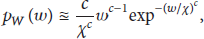
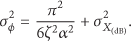
In Lemma 1, we can see that the random internodal distance and lognormal shadowing are now approximated with a single lognormal RV with certain mean and variance. Therefore, (7) is now reduced to $\Theta \cong ZR$ , where Z is a lognormal RV with mean as in (14) and variance, as in (16), and R is the Rician RV with Rice factor κ. Next, we approximate the lognormal-Rice product distribution by another lognormal RV, $U=\mathrm{1}{\mathrm{0}}^{G/\mathrm{10}}$ , where G is associated normal RV; however, the closed-form PDF for their product is also prohibited. For this approximation, one method is to use the moment matching technique as shown in Lemma 1, or the other method is to use the moment generating function (MGF) method. We use the latter approach.

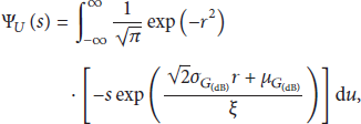
In MGF-based method, the MGF of the approximating lognormal RV, U, and the MGF of the lognormal-Rice RVs, $ZR$ , are equated at two distinct points to find the mean and variance of U. To proceed further, the PDF of the approximating lognormal RV, U, can be expressed as

$$\begin{array}{cc}& p_U\left(u\right)={{\displaystyle \int }}_{-\infty }^{\infty }\frac{\zeta }{u{\sigma }_{G_{\left(\mathrm{d}\mathrm{B}\right)}}\sqrt{\mathrm{2}\pi }}\exp \left\{\frac{-{\left(\zeta \hspace{0.17em}{\mathrm{l}\mathrm{o}\mathrm{g}}_{e}u-{\mu }_{G_{\left(\mathrm{d}\mathrm{B}\right)}}\right)}^{\mathrm{2}}}{\mathrm{2}{\sigma }_{G_{\left(\mathrm{d}\mathrm{B}\right)}}^{\mathrm{2}}}\right\}\mathrm{d}u,\end{array}$$

(17)

where ${\mu }_{G_{(\mathrm{d}\mathrm{B})}}$ and ${\sigma }_{G_{(\mathrm{d}\mathrm{B})}}^{\mathrm{2}}$ are the mean and variance of the associated Gaussian RV, G, respectively. The MGF of U is given as

$$\begin{array}{cc}& {\Psi }_U\left(s\right)={{\displaystyle \int }}_{\mathrm{0}}^{\infty }\mathrm{e}\mathrm{x}\mathrm{p}\left(-su\right)p_U\left(u\right)\mathrm{d}u.\end{array}$$

(18)

After substitution, (18) can be rewritten as

$$\begin{array}{cc}& {\Psi }_U\left(s\right)={{\displaystyle \int }}_{-\infty }^{\infty }\frac{\mathrm{1}}{\sqrt{\pi }}\exp \left(-r^{\mathrm{2}}\right)\left[-s\exp \left(\frac{\sqrt{\mathrm{2}}{\sigma }_{G_{\left(\mathrm{d}\mathrm{B}\right)}}r+{\mu }_{G_{\left(\mathrm{d}\mathrm{B}\right)}}}{\xi }\right)\right]\mathrm{d}u,\end{array}$$

(19)

where $r=\left(\zeta \hspace{0.17em}{\mathrm{l}\mathrm{o}\mathrm{g}}_{e}u-{\mu }_{G_{(\mathrm{d}\mathrm{B})}}\right)/\sqrt{\mathrm{2}}{\sigma }_{G_{(\mathrm{d}\mathrm{B})}}$ . It can be noticed that a closed-form solution to (19) is prohibited. Whereas it is difficult to find the MGF in closed-form, by applying numerical integration, it can be computed. In numerical integration, the integral is estimated by an approximate sum where the summation is defined by specific weights. A closer look at (19) yields a similarity to the Hermite polynomial, where general form for Hermite polynomial is given as

$$\begin{array}{cc}& H_n\left(x\right)={\left(-\mathrm{1}\right)}^n\exp \left(x^{\mathrm{2}}\right)\frac{d^n}{d{x}^n}\exp \left(-x^{\mathrm{2}}\right),\end{array}$$

(20)

where it takes the integral form as follows:

$$\begin{array}{cc}& {{\displaystyle \int }}_{-\infty }^{\infty }f\left(x\right)x^n\exp \left(-x^{\mathrm{2}}\right)\mathrm{d}x.\end{array}$$

(21)

The MGF in (19) also takes the form of a Hermite polynomial, which can be computed by applying Gauss-Hermite numerical integration method as

$$\begin{array}{cc}& {\Psi }_U\left(s;{\mu }_{G_{\left(\mathrm{d}\mathrm{B}\right)}},{\sigma }_{G_{\left(\mathrm{d}\mathrm{B}\right)}}\right)={\displaystyle \sum }_{h=\mathrm{1}}^H\frac{w_h}{\sqrt{\pi }}\exp \left[-s\exp \left(\frac{\sqrt{\mathrm{2}}{\sigma }_{G_{\left(\mathrm{d}\mathrm{B}\right)}}{a}_h+{\mu }_{G_{\left(\mathrm{d}\mathrm{B}\right)}}}{\xi }\right)\right],\end{array}$$

(22)

where Hermite integration order, H, is used to achieve better estimation of the MGF of U; the larger the value of H the better the estimate. $w_h$ is the weight corresponding to the abscissas, $a_h$ , and $\xi =\mathrm{10}/\mathrm{l}\mathrm{n}\mathrm{10}$ is a constant for scaling. In [25], weights, abscissas, and the values for H can be found in a tabulated form. Similarly, the PDF of lognormal-Rice RV, $\Theta =ZR$ , where Z is the lognormal RV with mean ${\mu }_{\varphi }$ and variance ${\sigma }_{\varphi }^{\mathrm{2}}$ and R is the Rician RV with Rice-factor κ, takes the integral form

$$\begin{array}{cc}& p_{\Theta }\left(\theta \right)={{\displaystyle \int }}_{\mathrm{0}}^{\infty }\frac{\mathrm{2}\theta \left(\kappa +\mathrm{1}\right)}{z^{\mathrm{2}}}\exp \left\{-\kappa -\left(\kappa +\mathrm{1}\right)\frac{\theta }{z^{\mathrm{2}}}\right\}·I_{\mathrm{0}}\left(\frac{\mathrm{2}\theta }{z}\sqrt{\kappa \left(\kappa +\mathrm{1}\right)}\right)p_Z\left(z\right)\mathrm{d}z,\end{array}$$

(23)

where $I_{\mathrm{0}}$ is the modified Bessel function of zero order and $p_Z(z)$ is given in (11). The MGF of the lognormal-Rice RV, Θ, after applying Gauss-Hermite integration, can be written as

$$\begin{array}{cc}& {\Psi }_{\Theta }\left(s;{\mu }_{\varphi },{\sigma }_{\varphi },\kappa \right)={\displaystyle \sum }_{h=\mathrm{1}}^H\frac{w_h\left(\mathrm{1}+{\kappa }_R\right)/\sqrt{\pi }}{\mathrm{1}+{\kappa }_R+s\exp \left(\left(\sqrt{\mathrm{2}}{\sigma }_{\varphi }{a}_h+{\mu }_{\varphi }\right)/\xi \right)}·\exp \left(-\frac{s{\kappa }_R\exp \left(\left(\sqrt{\mathrm{2}}{\sigma }_{\varphi }{a}_h+{\mu }_{\varphi }\right)/\xi \right)}{\mathrm{1}+{\kappa }_R+s\exp \left(\left(\sqrt{\mathrm{2}}{\sigma }_{\varphi }{a}_h+{\mu }_{\varphi }\right)/\xi \right)}\right).\end{array}$$

(24)

The mean and variance parameters, ${\mu }_{G_{(\mathrm{d}\mathrm{B})}}$ and ${\sigma }_{G_{(\mathrm{d}\mathrm{B})}}^{\mathrm{2}}$ , of the approximated lognormal RV can be calculated by equating (22) and (24) as

$$\begin{array}{cc}& {\Psi }_U\left(s_i;{\mu }_{G_{\left(\mathrm{d}\mathrm{B}\right)}},{\sigma }_{G_{\left(\mathrm{d}\mathrm{B}\right)}}\right)={\Psi }_{\Theta }\left(s_i;{\mu }_{\varphi },{\sigma }_{\varphi },\kappa \right)\hspace{1em}i=\mathrm{1},\mathrm{2}.\end{array}$$

(25)

The two nonlinear equations can be solved using a numerical routine. As the right-hand side comprises all known variables, solving for $s_{\mathrm{1}}$ and $s_{\mathrm{2}}$ we get the desire moments of U. Hence, we can say that the impact of three RVs on a single path of transmission can be approximated with a single lognormal RV. We now focus on a more general arrangement where multiple nodes are transmitting the same message to a node at the next level. In this case, the received power is the sum of RVs from all different transmission paths, each following independent distribution due to distinct σ of each RV. If $A=\left|{\mathcal{M}}_{n-\mathrm{1}}\right|$ is the number of DF nodes at level $n-\mathrm{1}$ then

$$\begin{array}{cc}& {\displaystyle \sum }_{\mathcal{l}=\mathrm{1}}^A\left\{{\Theta }_{\mathcal{l}}\right\}={\displaystyle \sum }_{\mathcal{l}=\mathrm{1}}^A\left\{\frac{X_{\mathcal{l}}{R}_{\mathcal{l}}}{W_{\mathcal{l}}}\right\}.\end{array}$$

(26)

As each Θ is approximated as a lognormal RV, U, the received power at a node at level n is the sum of A independent but nonidentical lognormal RVs. We again use the MGF transformation method here as the distribution for sum of lognormal RVs does not exist in a closed-form [18]. In MGF domain, the summation of RVs is represented as the product of their individual MGFs. The MGF for the sum of lognormal RVs is given as

$$\begin{array}{cc}& {\displaystyle \sum }_{\mathcal{l}=\mathrm{1}}^A{\Psi }_{U_{\mathcal{l}}}\left(s_i;{\mu }_{G_{\left(\mathrm{d}\mathrm{B}\right)}^{\left(\mathcal{l}\right)}},{\sigma }_{G_{\left(\mathrm{d}\mathrm{B}\right)}^{\left(\mathcal{l}\right)}}\right)={\displaystyle \prod }_{\mathcal{l}=\mathrm{1}}^A{\Psi }_{U_{\mathcal{l}}}\left(s_i;{\mu }_{\mathcal{l}},{\sigma }_{\mathcal{l}}\right)\hspace{1em}i=\mathrm{1},\mathrm{2},\end{array}$$

(27)

where ${\mu }_{G_{(\mathrm{d}\mathrm{B})}^{(\mathcal{l})}},{\sigma }_{G_{(\mathrm{d}\mathrm{B})}^{(\mathcal{l})}}$ are the mean and standard deviation of each individual lognormal RV, U. Furthermore, by using (25) we can rewrite (27) as

$$\begin{array}{cc}& {\displaystyle \sum }_{\mathcal{l}=\mathrm{1}}^A{\Psi }_{U_{\mathcal{l}}}\left(s_i;{\mu }_{G_{\left(\mathrm{d}\mathrm{B}\right)}^{\left(\mathcal{l}\right)}},{\sigma }_{G_{\left(\mathrm{d}\mathrm{B}\right)}^{\left(\mathcal{l}\right)}}\right)={\displaystyle \prod }_{\mathcal{l}=\mathrm{1}}^A{\Psi }_{{\Theta }_{\mathcal{l}}}\left(s_i;{\mu }_{\mathcal{l}},{\sigma }_{\mathcal{l}},{\kappa }_{\mathcal{l}}\right)\hspace{1em}i=\mathrm{1},\mathrm{2},\end{array}$$

(28)

where ${\mu }_{\mathcal{l}}$ and ${\sigma }_{\mathcal{l}}$ are the mean and standard deviation of the $\mathcal{l}$ th lognormal-Rice RV, Θ, and ${\kappa }_{\mathcal{l}}$ is the Rice-factor. Therefore, we can approximate sum of A lognormal-Rice RVs, $\{U_{\mathrm{1}},U_{\mathrm{2}},\dots ,U_A\}$ , by a single lognormal RV, $\mathcal{J}=\mathrm{1}{\mathrm{0}}^{\mathcal{L}/\mathrm{10}}$ , such that $\mathcal{J}~\mathrm{l}\mathrm{o}\mathrm{g}\mathcal{N}({\mu }_{\mathcal{L}},{\sigma }_{\mathcal{L}}^{\mathrm{2}})$ . The approximated single lognormal RV $\mathcal{J}$ 's MGF is given by

$$\begin{array}{cc}& {\Psi }_{\mathcal{J}}\left(s;{\mu }_{\mathcal{L}},{\sigma }_{\mathcal{L}}\right)={\displaystyle \sum }_{h=\mathrm{1}}^H\frac{w_h}{\sqrt{\pi }}\exp \left[-s\exp \left(\frac{\sqrt{\mathrm{2}}{\sigma }_{\mathcal{L}}{a}_h+{\mu }_{\mathcal{L}}}{\xi }\right)\right].\end{array}$$

(29)

Here ${\mu }_{\mathcal{L}}$ and ${\sigma }_{\mathcal{L}}$ are the logarithmic mean and standard deviation of lognormal RV $\mathcal{J}$ . By equating the two nonlinear equations, that is, (28) and (29), these quantities can be calculated by using a numerical routine.

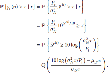
After deriving the PDF of RVs, we now concentrate to derive the success probability of a node in Figure 1. To find that a node has decoded the message correctly, the received SNR should be greater than or equal to a decoding threshold, τ. To be specific, the received SNR of a node i at level n is determined by the distribution of RV $\mathcal{J}$ , now given as

$$\begin{array}{cc}& {\gamma }_i\left(n\right)=\frac{P_t}{{\sigma }_N^{\mathrm{2}}}{\displaystyle \sum }_{\mathcal{l}=\mathrm{1}}^A\left\{{\Theta }_{\mathcal{l}}\right\}=\frac{P_t}{{\sigma }_N^{\mathrm{2}}}{\mathcal{J}}^{\left(i\right)}.\end{array}$$

(30)

This alters the conditional probability in (5) as

$$\begin{array}{cc}& \mathbb{P}\left\{{\gamma }_i\left(n\right)>\tau \hspace{0.17em}|\hspace{0.17em}\epsilon \right\}=\mathbb{P}\left\{\frac{P_t}{{\sigma }_N^{\mathrm{2}}}{\mathcal{J}}^{\left(i\right)}>\tau \hspace{0.17em}|\hspace{0.17em}\epsilon \right\}=\mathbb{P}\left\{\frac{P_t}{{\sigma }_N^{\mathrm{2}}}\mathrm{1}{\mathrm{0}}^{{\mathcal{L}}^{\left(i\right)}/\mathrm{10}}\ge \tau \right\}=\mathbb{P}\left\{{\mathcal{L}}^{\left(i\right)}\ge \mathrm{10}\log \left(\frac{{\sigma }_N^{\mathrm{2}}\tau }{P_t}\right)\right\}=Q\left(\frac{\mathrm{10}\log \left({\sigma }_N^{\mathrm{2}}\tau /P_t\right)-{\mu }_{{\mathcal{L}}^{\left(i\right)}}}{{\sigma }_{{\mathcal{L}}^{\left(i\right)}}}\right),\end{array}$$

(31)

where Q-function denotes the tail probability, which is of our interest in determining the outage probability. It is important to notice that the success probability depends on the transimit power, $P_t$ , decoding threshold, τ, and calculated ${\mu }_{\mathcal{L}}$ and ${\sigma }_{\mathcal{L}}$ . In a certain state, the one-hop transition probability is given by (6), whereas the probability to decode the message signal for a single node is given by (31). Similarly, for all nodes in level n the same method is repeated which will populate our transition probability matrix, T. The Perron-Frobenius theorem is then applied on T to determine the one-hop success probability. Our workflow in this paper can be logged as shown in Table 1.

Table 1

Work flow of deriving the PDF of SNR at a node.

Expression	Transformation	Process	Method used
$$\mathrm{\Theta }=\frac{XR}{W}$$	$$W=\frac{\mathrm{1}}{Y}$$	W Weibull RV is transformed into inverse Weibull RV Y	Variable transformation
	$$Z=XY$$	The product distribution in Lemma 1	Moment matching approach
	$$\mathrm{\Theta }=ZR$$	The product distribution	MGF-based method
	$${\mathrm{\Psi }}_U\left(s;{\mu }_{G_{(\mathrm{d}\mathrm{B})}},{\sigma }_{G_{(\mathrm{d}\mathrm{B})}}\right)={\mathrm{\Psi }}_{\mathrm{\Theta }}\left(s;{\mu }_{\varphi },{\sigma }_{\varphi },{\kappa }_R\right)$$	Lognormal-Rice RV approximation	MGF-based method
$${{\displaystyle \sum }}_{i=\mathrm{1}}^A\left\{{\mathrm{\Theta }}_i\right\}={{\displaystyle \sum }}_{i=\mathrm{1}}^A\left\{\frac{X_i{R}_i}{W_i}\right\}$$	$${{\displaystyle \sum }}_{i=\mathrm{1}}^A\left\{{\mathrm{\Theta }}_i\right\}$$	Sum of A lognormal RVs	MGF-based approach
	$${{\displaystyle \sum }}_{i=\mathrm{1}}^A\left\{U_i\right\}=\prod _{\mathcal{l}=\mathrm{1}}^A{\mathrm{\Psi }}_{{\mathrm{\Theta }}_{\mathcal{l}}}\left(s_i;{\mu }_{\mathcal{l}},{\sigma }_{\mathcal{l}}\right)$$	The sum into product conversion	MGF-based approach
	$\mathcal{J}={{\displaystyle \sum }}_{i=\mathrm{1}}^A\left\{U_i\right\}$	Sum approximation as a single lognormal RV $\mathcal{J}$	MGF-based approach
	$$\mathcal{J}=\prod _{\mathcal{l}=\mathrm{1}}^A{\mathrm{\Psi }}_{{\mathrm{\Theta }}_{\mathcal{l}}}\left(s_i;{\mu }_{\mathcal{l}},{\sigma }_{\mathcal{l}},{\kappa }_{\mathcal{l}}\right)$$	The final lognormal RV as a product of A lognormal-Rice RVs	MGF-based approach
Received SNR at a node i	$${\gamma }_i\left(n\right)=\frac{P_t}{{\sigma }_N^{\mathrm{2}}}{\mathcal{J}}^{(i)}$$

5. Results and Performance Analysis

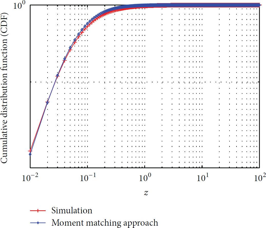
In this section, we validate our analytical models and present some numerical results for various sets of parameters. At first we plot the comparison between the cumulative distribution function (CDF) of the approximated lognormal RV and network simulations to determine the accuracy of model proposed in Lemma 1. Monte Carlo simulation of the product of lognormal and inverse Weibull RV is performed and compared with the proposed moment matching method. In simulation, the inverse Weibull and lognormal RVs are generated separately, multiplied, and averaged over $\mathrm{1}{\mathrm{0}}^{\mathrm{7}}$ iterations of Monte Carlo. From Figure 2, we can see that the CDF obtained for both the moment matching approach and network simulations is in a good match, hence, providing an accuracy of approximation proposed.

Figure 2

Comparison of CDFs of theoretical and simulation approaches, $\beta =\mathrm{2}$ , $L=\mathrm{2}$ , ${\mu }_{\varphi }=\mathrm{0}\hspace{0.17em}\mathrm{d}\mathrm{B}$ , ${\sigma }_{\varphi }=\mathrm{6}\hspace{0.17em}\mathrm{d}\mathrm{B}.$

Figure 3 shows the one-hop success probability, ρ, for both analytical model and simulations, for $\mathrm{3}$ nodes in a level. The analytical values of one-hop success is the Perron-Frobenius eigenvalue obtained by forming the transition probability matrix, T, where each value of T is evaluated using (6). On the other hand, for simulations, the one-hop success probability is calculated using the fact that at least one node in a level decodes the message signal correctly, where N nodes are randomly generated in adjacent square regions of $L=\mathrm{5}$ . The normalized SNR margin, ${\rm Y}=P_t/\tau$ , is used to depict the results obtained at each hop and then averaged over ten million iterations. It can be noticed that the simulation results are quite close to the results of the proposed analytical model. Further notice that as the number of nodes, N, increases, the one-hop success probability also increases, indicating an increased diversity gain. A small SNR margin is required by the system to achieve a certain probability of success as the number of N increases. For all the results, we assume identical values of σ and Rice K-factor, κ for signals from multiple transmitting nodes, along with path loss exponent, $\beta =\mathrm{2}$ .

Figure 3

Simulation versus analytical results for $N=\mathrm{3}$ , $L=\mathrm{5}$ , $\beta =\mathrm{2}$ , $\sigma =\mathrm{6}\hspace{0.17em}\mathrm{d}\mathrm{B}$ .

In Figure 4, the effect of shadowing in terms of σ is shown on the one-hop success probability, ρ. It can be noticed that at low SNR margins, an increase in σ increases ρ. This is because the variations in the received power across a certain mean are defined by σ, and the mean in turn is defined by the path loss exponent; the higher the variations, the higher σ.

Figure 4

Varying standard deviation for different values of path loss exponent $N=\mathrm{3}$ , $L=\mathrm{2}$ .

This implies that at low SNR margin the system is path loss limited and as the signal propagates through the wireless medium, the path loss is dominant, thus suppressing the effect of shadowing severity, and we might get a favourable response for an increase in σ, that is, increase in one-hop success probability. On the other hand, path loss is compensated as the SNR margin increases and the shadowing severity starts to play its role. Hence, in Figure 2 inset, reverse phenomenon is depicted. As the SNR margin attains higher values, the path loss decreases and only the severity of shadowing causes the probability of success to drop for larger values of σ. Furthermore, from the same figure it can be noticed that as the path loss exponent, β, is increased, an overall degradation in the performance of the system can be observed.

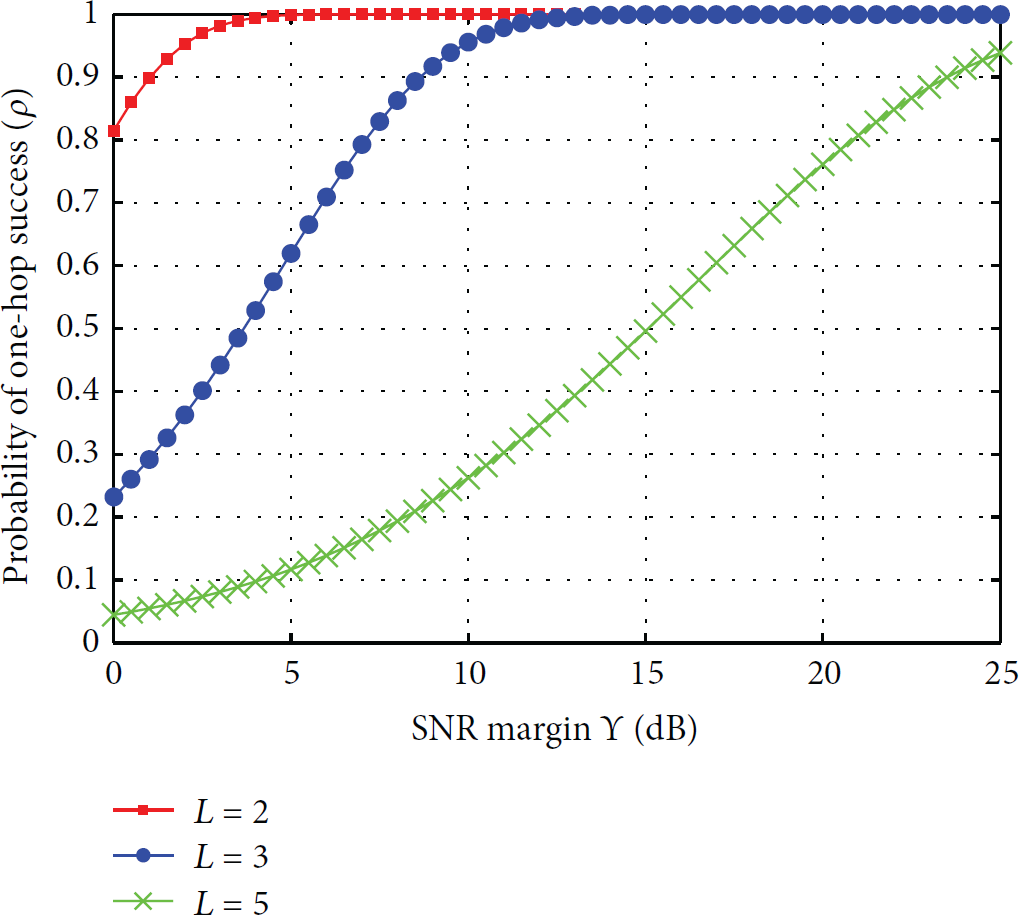
The behavior of the path loss can also be attributed from Figure 5, where an increase in length, L, of the region increases the average distance between two hops, whereas number of nodes $N=\mathrm{3}$ remains fixed. This results in larger signal attenuation and hence the probability of success drops.

Figure 5

Success probability for different value of region length, $N=\mathrm{3}$ , $\beta =\mathrm{2}$ .

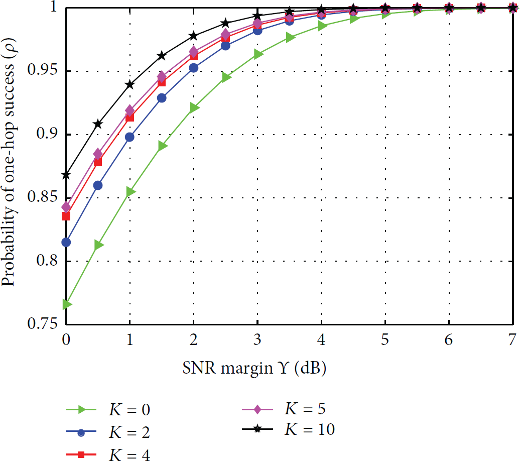
In Figure 6, the effect of Rice K-factor, κ, is observed by keeping $\sigma =\mathrm{6}\hspace{0.17em}\mathrm{d}\mathrm{B}$ . We consider a fixed network size, $L=\mathrm{2}$ , and a fixed number of nodes, $N=\mathrm{3}$ , to observe the effect of κ. As the SNR margin attains higher values, the one-hop success probability increases as we increase the value of K-factor. It can be noticed that as much as $\mathrm{2}\hspace{0.17em}\mathrm{d}\mathrm{B}$ of additional SNR margin is required if the environment becomes NLOS ( $\kappa =\mathrm{0}$ , Rayleigh fading) as compared to LOS when $\kappa =\mathrm{10}$ . The deployment of a sensor network depends highly on the type of environment and the SNR margin should be adjusted accordingly for a desired quality of service (QoS).

Figure 6

Success probability versus SNR margin for varying K-factor.

The performance of the multihop strip networks depends on the probability of a message to successfully reach a certain destination without going into absorbing state. This end-to-end success probability is defined by QoS parameter, η, which is important to determine the coverage range of the network. For example, if we are required to reach a certain distance with $\mathrm{80}\%$ QoS then $\eta =\mathrm{0.8}$ . The message signal in our model can propagate a maximum of n-hops until the killing occurs, as shown in (4). For a fixed set of network parameters (path loss exponent, β, region length, L, and transmit power, $P_t$ ) ρ has a fixed value. Hence the QoS parameter sets an upper bound to the success probability of n-hop count; that is, $\eta \le {\rho }^n$ . The maximum number of hops the message can travel is given by

$$\begin{array}{cc}& n\le \frac{\ln \eta }{\ln \rho }.\end{array}$$

(32)

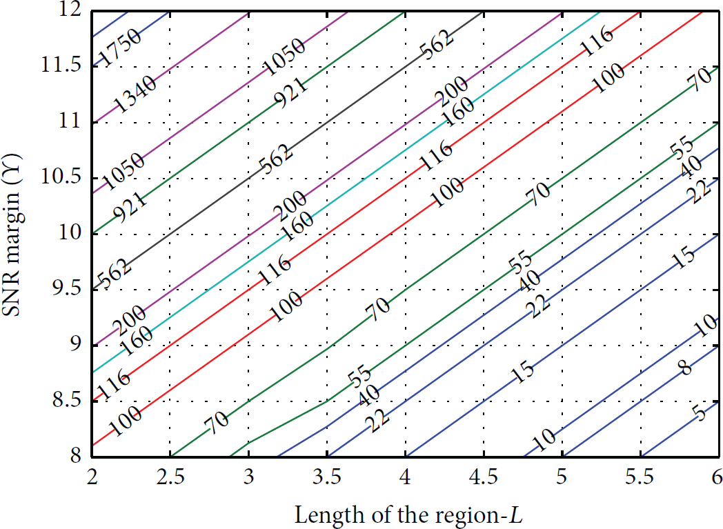
To calculate the network coverage range, the product of n (obtained from (32)) and the length of the region, L, will provide the maximum distance a message can propagate while achieving a certain QoS. In Figure 7, the coverage range contours against length of the region L and SNR margin, Υ, are illustrated for $\eta =\mathrm{0.85}$ and $N=\mathrm{2}$ . The drop in maximum hop count as the value of L stretches depicts the distinct effect of path loss, as a fact that we are increasing the average distance between the hops. From this plot, a network designer can set various different combination of network parameters to attain certain value of network coverage. A network with latency constraint can achieve a given coverage range with fewer number of hops at the expense of high SNR margin (transmit power, $P_t$ ), whereas networks with power constraint can achieve the same coverage by reducing the hop size. For instance, if coverage range of $\mathrm{200}$ is desired, then former performance (delay-limited) can be achieved by using $L=\mathrm{4.6}$ and ${\rm Y}=\mathrm{11.5}\hspace{0.17em}\mathrm{d}\mathrm{B}$ . However, for the latter performance (energy-efficiency), $L=\mathrm{2}$ and ${\rm Y}=\mathrm{9}\hspace{0.17em}\mathrm{d}\mathrm{B}$ can be used.

Figure 7

Coverage range for the extended strip network for $N=\mathrm{2}$ , $\sigma =\mathrm{6}\hspace{0.17em}\mathrm{d}\mathrm{B}$ , and $\eta =\mathrm{0.85}$ .

6. Conclusions and Future Work

In this paper, a strip-shaped extended network is studied by developing a discrete-time Markov chain model. We analysed the network under the impact of three random processes, that is, lognormal shadowing, Rice fading, and Weibull random distance. We derived the success probability of all nodes in adjacent regions using a three-step process. First, we derived a product distribution between inverse Weibull RV and lognormal RV and approximated it as another lognormal RV using a moment matching approach. The MGF-based method along with Gauss-Hermite integration is used to determine the product of resulting lognormal RV with Rice RV, where the sum of these lognormal-Rice RVs is approximated with a single lognormal RV. Corresponding to the Markov chain with quasi-stationary distribution and the derived coverage probability, a transition matrix is derived using a simple binomial equation. A specific SNR margin is quantified for the network coverage range of the network as a function of different parameters. In future, the model can be studied by removing the hop boundary constraints and to analyse the network for random number of nodes at each level. Furthermore, the effects of shadowing correlation can be included, which will be another step forward towards the idea of achieving a more practical model.