A Grid-Based Linear Least Squares Self-Localization Algorithm in Wireless Sensor Network

Abstract

Self-localization is one of the key technologies in the wireless sensor networks (WSN). Some traditional self-localization algorithms can provide a reasonable positioning accuracy only in a uniform and dense network, while for a nonuniform network the performance is not acceptable. In this paper, we presented a novel grid-based linear least squares (LLS) self-localization algorithm. The proposed algorithm uses the grid method to screen the anchors based on the distribution characteristic of a nonuniform network. Furthermore, by taking into consideration the quasi-uniform distribution of anchors in the area, we select suitable anchors to assist the localization. Simulation results demonstrate that the proposed algorithm can greatly enhance the localization accuracy of the anonymous nodes and impose less computation burden compared to traditional Trilateration and Multilateration.

1. Introduction

When we monitor a great forest in a dry weather, we would like to know which trees are more likely to catch fire. These localization problems are also important in environment detecting, animal tracker, wisdom agriculture, and so on. Now with the wild deployment of wireless sensor networks (WSN), we can do these monitoring and detecting jobs with WSN. And during this process, the first thing we should do still is to get the location of WSN node itself, and then we could know where the events happened.

Based on measuring the distance between the nodes or not, we can classify the self-localization algorithms to range-based and range-free. As compared to the range-based algorithm, the range-free algorithm has many advantages, including simpler hardware, lower power consumption, and more power in noise resistance. But the main disadvantage of range-free algorithms is big errors. The localization error and communication range between nodes have same order of magnitude, which could be a few tens of meters. If we can improve the localization accuracy, it will be better for many implementations. For example, when we monitor the geologic structure by WSN, higher localization accuracy could lead us to build a road on a solid ground but not the place with a sandpit underground which is only 10 meters away. Similarly, if we can point out which tree is the nest of the pest, we do not need to spray poison pesticides to the whole hillside. So we can see that precise localization will help us to achieve the real sense of precise control.

There are numerous classical range-free localization algorithms such as DV-Hop, convex programming, MDS-MAP, and DHL. Generally, the range-free algorithm can be divided into three steps.

• (1)

Estimate the distance between the sensor node and sink node.

(2)

Calculate the localization of the sensor node with Trilateration.

(3)

Optimize the result we get in the last step with iterative method.

Within these three steps, there are two main approaches to improve the precision of range-free localization algorithm. The first is increasing the precision of distance estimation. As in literature [1], it was studied on nonuniformly distributed WSN. Based on the hop count to the anchor, the network was divided into three areas as CR (Concentric Ring), CG (Centrifugal Gradient), and DG (Distorted Gradient). In each area, different method was used to reduce the error of the distance estimate. In [2], the authors think that the normal Gaussian probability density function cannot be used to estimate the distance between sensor nodes and anchors in two-dimensional random distribution networks. And the author proposed the biggest distance estimate method based on the greedy algorithm. In [3], the authors study the expected hop count in different WSN which has different parameters. Based on these analyses, authors deduced the mathematical expression of the hop count. With this method, it can greatly enhance the estimation precision of the distance between the sensors to the anchors. Another way to promote the localization precision is increasing the number of the iterations within Step 3. With this method, the distance error will be decreased, but at the same time it will increase the complexity of algorithm and the amount of calculation. Furthermore, it is hard to predict the right number of iterations, so the uncertainty of the result will increase. For these reasons, it is restricted to use iterations in practice [4].

Unlike the approaches as showed above, we pay more attention to Step 2: calculate the localization of the sensor node with Trilateration localization algorithm. In general, Trilateration-localization or Multilateral-localization method will be used here. We found that even we work hard to get a more accurate estimate value of the distance, but if we use some bad anchors in Trilateration or Multilateration, the result would be still far away from perfect. On the contrary, even the distance estimate is not perfect if we choose the right anchors in calculation method and then the result would be better. But now the key problem is which anchors are the right anchors? What we do is try to figure out what a right anchor is and how to select them from the total anchors. With the help of these right anchors in calculation method, we can improve the performance of localization algorithm.

As we know, Trilateration has small algorithm computation. On the other side, in this method only the three main anchors’ information is used, so it is difficult to promote the localization precision. But if we use more anchors’ information to promote the precision of localization, then more computing resources will be required. Reference [5] indicates that the error of the distance estimate will increase with the increase of the hop count. Reference [6] explained that we can promote the localization precision by deleting some anchors which have large errors. Reference [7] shows that the precision of unknown nodes is affected by spatial distribution of the involved anchors. The more the uniformity of the anchors distributed is, the more accurate the result will be. The simulation result of [8] also shows that the uniform distribution of the anchors can greatly improve the positioning performance.

This paper proposed a grid-based linear least squares (LLS) self-localization algorithm. The algorithm will fully consider the character of the nonuniformity networks and uses the grid method to select the anchors. In this algorithm, we will delete the anchors which have bigger error and bad distribution and at the same time choose the appropriate anchors to make the distribution of the anchors be more even. Simulation results show that our algorithm has higher localization accuracy and has lower computational cost, compared to the traditional Trilateration and Multilateration.

2. Grid-Based Linear Least Squares (LLS) Self-Localization Algorithm

References [5–8] show that Multilateration has higher localization accuracy because Multilateration involves more anchors in localization method and uses least squares estimation to decrease the influence of the errors. But as the number of the anchors increases, Multilateration needs more bandwidth to transmit data and more computation and energy consumption. Furthermore, in range-free localization algorithm, the error of the distance estimate will increase as the hop count ascends. Therefore, using more anchors in localization means that we are likely to involve more anchors which have larger distance estimated errors. These errors will seriously influence the localization accuracy. As we know, the uniformity of the anchors distribution has a very important effect on the localization accuracy.

In summary, the numbers and distribution of the anchors are the key factors to improve the precision of self-localization. Therefore, we can select a part of the anchors which have small error and proper position through deleting the anchors with bigger errors and bad distribution. With this process, we can promote the localization precision and decrease the calculation and energy consumption. Meanwhile, this is helpful to prolong the life-time of WSN.

We at least need three anchor nodes for locating in 2D orientation as shown in Figure 1(a). But, due to distance measurement errors, the intersection of the localization circle of the three anchor nodes is not a point but an area, as shown in Figure 1(b). Then, the problem of promoting the accuracy of localization is transformed into the problem of making the area as small as possible. About this problem, we use the proof proceeding of [9] and promoted it to multianchor nodes cases.

Figure 1

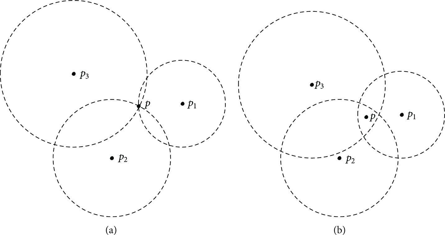
Error area in localization with three anchor nodes.

However, in Trilateration or in Multilateration, it at least needs three anchor nodes to locate the unknown node in 2D orientation, as shown in Figure 1(a). But, due to distance estimation error, the intersection of the localization circle of the three anchor nodes is not a point but an area, as shown in Figure 1(b). Then, the problem of improving the accuracy of localization is transformed into the problem of making the overlap area as small as possible. To this problem, we use the idea of [9] and promote it into multianchor nodes cases.

To simplify the problem and without loss of generality, we first assume that the distance estimation error between every anchor and unknown node is independent. And the localization error of the anchor itself is much less than the distance estimation error between anchor and the unknown node in range-free system, so we will neglect the position error of the anchor. Under normal circumstances, the distance error is much less than the distance between the anchor and the unknown node, so we only use a simple constant to express the distance error.

We first analyze the condition which only has three anchor nodes. We assume the three anchor nodes as $p_i=(x_i,y_i)$ , $i=\mathrm{1,2},\mathrm{3}$ , in two-dimensional space. The real location of the unknown node is $p=(x_{\mathrm{0}},y_{\mathrm{0}})$ and the real distances between the unknown node p and the anchor node $p_i$ are $r_i=d(p,p_i)$ , $i=\mathrm{1,2},\mathrm{3}$ . And we assume that the distance error range is in the range of $(\mathrm{0},\epsilon )$ . So we can draw a circle $S_p$ of radius ε. The area of this circle is $\left\{(x,y)\hspace{0.17em}|\hspace{0.17em}(x-x_{\mathrm{0}}{)}^{\mathrm{2}}+(y-y_{\mathrm{0}}{)}^{\mathrm{2}}={\epsilon }^{\mathrm{2}}\right\}$ . This circle can be used to express the error area of trilateration. As we set $l_{p,p_i}$ as the straight line cross points p and $p_i$ , then the line intersects the circle $S_p$ at two points $q_{p_i,\mathrm{1}}$ and $q_{p_i,\mathrm{2}}$ . In these two points, $q_{p_i,\mathrm{1}}$ is close to point P and $q_{p_i,\mathrm{2}}$ is a little farther. When we have three anchors, we can draw the tangent line of circle $S_p$ with the intersection points $q_{p_{\mathrm{1}},\mathrm{2}}$ , $q_{p_{\mathrm{2}},\mathrm{2}}$ , and $q_{p_{\mathrm{3}},\mathrm{2}}$ . These three tangent lines form a circumscribed triangle of circle $S_p$ , and we call it as $C_p$ . Because the distance error is far smaller than $r_i$ in range-free systems, we can transform the area of the overlapping portion of three localization circles to the area of $C_p$ . As shown in Figure 2, the method of calculating the area of $C_p$ can be broken up into calculating the area of three triangles $\Delta ApB$ , $\Delta BpC$ , and $\Delta CpA$ , respectively, and then adding three areas together.

Figure 2

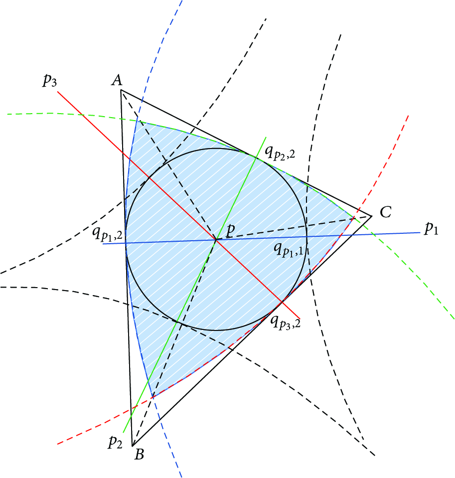
Analysis of location error.

As $a_{i,j}$ is the angle between vector $\overrightarrow{p{q}_{p_{\mathrm{1}},\mathrm{2}}}$ and $\overrightarrow{p{q}_{p_{\mathrm{2}},\mathrm{2}}}$ , we can get the area of the triangle $\Delta ABC$ from formula (1). At this point, we express this area as $\text{area}(C_p)$ :

$$\begin{array}{ll}\text{area}\left(C_p\right)& =\frac{\mathrm{1}}{\mathrm{2}}\epsilon \left[\epsilon \tan \left(\frac{a_{\mathrm{12}}}{\mathrm{2}}\right)+\epsilon \tan \left(\frac{a_{\mathrm{31}}}{\mathrm{2}}\right)\right]\\ & \hspace{1em}+\frac{\mathrm{1}}{\mathrm{2}}\epsilon \left[\epsilon \tan \left(\frac{a_{\mathrm{12}}}{\mathrm{2}}\right)+\epsilon \tan \left(\frac{a_{\mathrm{23}}}{\mathrm{2}}\right)\right]\\ & \hspace{1em}+\frac{\mathrm{1}}{\mathrm{2}}\epsilon \left[\epsilon \tan \left(\frac{a_{\mathrm{23}}}{\mathrm{2}}\right)+\epsilon \tan \left(\frac{a_{\mathrm{31}}}{\mathrm{2}}\right)\right]\hspace{1em}\text{or}\\ \text{area}\left(C_p\right)& ={\epsilon }^2\left[\tan \left(\frac{a_{12}}{2}\right)+\tan \left(\frac{a_{23}}{2}\right)+\tan \left(\frac{a_{31}}{2}\right)\right].\end{array}$$

(1)

Because $\tan {\left(x\right)}^{\mathrm{\prime \prime }}=\mathrm{2}\tan (x)(\mathrm{1}+\tan (x))\ge \mathrm{0}$ and $a_{12},a_{23},a_{31}\ne \mathrm{0}$ , the area $\text{area}(C_p)$ is a strictly convex function and we can get the consequence as follows:

$$\begin{array}{ll}\text{area}\left(C_p\right)& ={\epsilon }^2\left[\tan \left(\frac{a_{12}}{2}\right)+\tan \left(\frac{a_{31}}{2}\right)+\epsilon \tan \left(\frac{a_{23}}{2}\right)\right]\\ & \ge 3{\epsilon }^2\tan \left[\frac{1}{3}\left(\frac{a_{12}}{2}+\frac{a_{23}}{2}+\frac{a_{31}}{2}\right)\right]\\ & =3{\epsilon }^2\tan \left[\frac{\pi }{3}\right].\end{array}$$

(2)

The equality will hold up if $a_{12}=a_{23}=a_{31}=2\pi /3$ ; that is, if the three anchor nodes distributed as an equilateral triangle to the unknown node, the area $\text{area}(C_p)$ will be the smallest. That is to say, the localization error should be the minimum.

Similarly, when we use more anchors in node self-location, the area of circumscribed polygon $C_p$ can be structured by many triangles. For example, there are m anchor nodes involved in the process of localization; with (2) we get

$$\begin{array}{ll}\text{area}\left(C_p\right)& ={\epsilon }^2\left[\tan \left(\frac{a_{12}}{2}\right)+\tan \left(\frac{a_{23}}{2}\right)+\cdots +\tan \left(\frac{a_{m1}}{2}\right)\right],\\ & a_{12}+a_{23}+\cdots +a_{31}=2\pi .\end{array}$$

(3)

Like before, the area $\text{area}(C_p)$ is a strictly convex function, so we still can get that, while $a_{12}=a_{23}\cdots =a_{m1}=2\pi /m$ , $\text{area}(C_p)$ should be the minimum:

$$\begin{array}{ll}\text{area}\left(C_p\right)& ={\epsilon }^2\left[\tan \left(\frac{a_{12}}{2}\right)+\tan \left(\frac{a_{31}}{2}\right)+\epsilon \tan \left(\frac{a_{23}}{2}\right)\right]\\ & \ge m{\epsilon }^2\tan \left[\frac{1}{m}\left(\frac{a_{12}}{2}+\frac{a_{23}}{2}+\cdots +\frac{a_{m1}}{2}\right)\right]\\ & =m{\epsilon }^2\tan \left[\frac{\pi }{m}\right].\end{array}$$

(4)

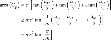
With the derivation process of the formulas, we can see that the localization error will be the minimum if and only if the angles which are formed by adjacent anchors and the unknown node are uniformly distributed. The major research of this paper is to study how to select the appropriate anchors to form such even angles and make the location error minimum at last. To solve this problem, we introduce a dynamic grid template to choose the right anchors for the unknown node. Anchors that have been chosen will evenly distribute to the unknown node. This process will improve the localization precision.

Based on this idea, we propose a grid-based linear least squares (LLS) self-localization algorithm. This algorithm still estimates the distance based on the hop count, so we do not need to change the hardware structure of the sensor nodes and the transmit process. So there should be minimal impact on existing systems. On this basis, we will still use Multilateration to localize the unknown nodes. But, in the process of selecting anchors, we will not choose total anchors whose packets the unknown nodes can receive. Alternatively, we delete the anchors whose hop count to the unknown nodes is larger than threshold $T_0$ and only use the rest of the anchors for Multilateration. Through this measure, we can reduce the probability to involve larger localization errors. In addition, the correlations of the anchors will increase with the decrease of their distance. But overcorrelation is not conducive to promote the localization accuracy and even can produce serious interference in some conditions. So we use grid method to delete the overcorrelation anchors. At last, we select well-distributed anchors from these remaining anchors based on the grid method once again and localize the unknown node through LLS.

In this paper, we call the nodes that need to be localized as unknown node, nodes which know their location and can help the unknown nodes to be localized as anchor nodes. Neighbor nodes are the nodes involved in one node's communication range. Current node means the node is being localized.

This algorithm is divided into 5 steps.

• (i)

Estimate the distance between unknown node and anchors.

(ii)

Make up grid and filter anchors.

(iii)

Determine the grid unit of the unknown node.

(iv)

Generate a set of the anchors which have even distribution to unknown node.

(v)

Localize the unknown node by the linear least square method.

Step 1 (estimate the distance between the unknown nodes and anchors).

There are many algorithms to get the distance between the unknown node and anchor. In order to make the result comparable, we use distance estimate method of DV-Hop all the time. DV-Hop is one of distributing localization algorithm sets, APS, which is proposed by Dragos Niculescu of Rutgers University. In DV-Hop, distance is estimated based on the hop count between anchor and unknown node. At first, it uses Distance Vector Algorithm or something like it to obtain the hop count from every unknown node and anchor to every anchor. Then, every anchor will calculate its own average distance of each hop based on the coordinates and the hop count to the other anchors, as shown in

$$\begin{array}{cc}& \text{HopSiz}{\text{e}}_i=\frac{{\sum }_{j\ne i}\sqrt{{\left(x_i-x_j\right)}^2+{\left(y_i-y_j\right)}^2}}{{\sum }_{j\ne i}{h}_j}.\end{array}$$

(5)

In formula (5), $(x_i,y_i),(x_j,y_j)$ is the coordinates of anchors i and j, $h_j$ is the number of the hops between anchors i and j   $(j\ne i)$ , and $\text{HopSiz}{\text{e}}_i$ is average distance of each hop to anchor i and it will be broadcast to whole networks. While unknown node receives the HopSize of the nearest anchor, it can calculate the estimated distance from itself to the anchors around.

Step 2 (set up the grid and filter the anchors).

For the unknown node, it could know the hop counts between the anchors and itself, after getting the information of the anchors. Then we can delete the anchors whose hop count to the current node is bigger than threshold $T_{\mathrm{0}}$ . This measure can effectively decrease the probability of greater errors involved in localization proceeding. After deleting the bad anchors, we can determine the distribution of the remainder anchors by their coordinates. We set $x_{\min }$ , $x_{\max }$ , $y_{\min }$ , and $y_{\max }$ as the minimum and maximum X and Y coordinate of the remainder anchors and set R as the communication range of the node. Then, $[x_{\min },x_{\max }]$ , $[y_{\min },y_{\max }]$ is the distribution range of the anchors to the X and Y axes. For ease of use, we properly regulate the start position of the grid. At first, we calculate the remainder of the span range of the anchors to R:

$$\begin{array}{cc}& x_{\text{residue}}=\mathrm{mod}\left(\left(x_{\max }-x_{\min }\right),R\right),\\ y_{\text{residue}}=\mathrm{mod}\left(\left(y_{\max }-y_{\min }\right),R\right).\end{array}$$

(6)

Then, we equally split the difference between the R and the remainder to both sides of the distributed span of the anchors:

$$\begin{array}{cc}& X_{\min }=x_{\min }-\frac{\left(R-x_{\text{residue}}\right)}{\mathrm{2}},\\ X_{\max }=x_{\max }+\frac{\left(R-x_{\text{residue}}\right)}{\mathrm{2}},\\ Y_{\min }=y_{\min }-\frac{\left(R-y_{\text{residue}}\right)}{\mathrm{2}},\\ Y_{\max }=y_{\max }+\frac{\left(R-y_{\text{residue}}\right)}{\mathrm{2}}.\end{array}$$

(7)

At last, we use $\left[X_{\min },X_{\max }\right],[Y_{\min },Y_{\max }]$ as the region of the grid and R as the interval to set up the grid system, as shown in Figure 3(a).

We can see that every unit of the grid is a square with each side of length R. And, as we know, if there are too many anchors in a unit, the accuracy of localization will be affected. So we choose the anchor with minimum hop to the unknown node as the representative anchor of the unit, and if more than one anchor has the same minimum hop count, we will only choose one anchor randomly.

Figure 3

Set up the grid and get the grid location of the unknown node.

Step 3 (determine the grid unit of the unknown node).

After setting up the grid, we need to determine the grid unit of the unknown node. Only if we know which grid unit the unknown node is located in, we can choose the appropriate anchors to form even distribution. In this paper, we draw on the idea of Min-Max localization algorithm and calculate the Min-Max range of every anchor based on the hop count from the anchor to the unknown node. Then choose a grid unit randomly among the overlapping area of every anchor's Min-Max range as the grid unit of current unknown node. The points of this process are shown in Figure 3(b).

Step 4 (generate uniformly distributed anchor set).

In this step, we choose the uniformly distributed anchors from the rest of the anchor set and used the unknown node as the center. Here we use a kind of mask.

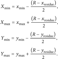
As shown in Figure 4, we first generate a square mask with each side of length $(2T_0+1)\times R$ and divide it into 8 parts ( $R1$ to $R8$ ). Then, we adjust the position of the mask and we make the grid unit of the unknown node as the center unit of the mask. Using the mask, every anchor can confirm which part it is located in. Then, the next question is how to choose the adequate anchors in every part, to make the selected anchors form a uniform distribution. Here we have 4 steps to perform.

• (1)

Count the number of anchors in every part. In order to ensure if there are enough anchors to be used in localization, we set that the minimum number of anchors that have been needed in localization process is $T_1$ and the minimum number of the anchors of all part is $R{\mathrm{8}}_{\min }$ . If $R{\mathrm{8}}_{\min }\times \mathrm{8}\ge T_1$ , we will choose $R{\mathrm{8}}_{\min }$ less hop count anchors in every partition and stop the mask process. Else, skip to Step 2.

(2)

Count the minimum number of anchors in the part set, Set1: $\{R1,R3,R5,R7\}$ and Set2: $\{R2,R4,R6,R8\}$ , recorded as $R\mathrm{4}\_{\mathrm{1}}_{\min \mathrm{1}}$ , $R\mathrm{4}\_{\mathrm{1}}_{\min \mathrm{2}}$ .

• (i)

  While $R\mathrm{4}\_{\mathrm{1}}_{\min \mathrm{1}}\ge R\mathrm{4}\_{\mathrm{1}}_{\min \mathrm{2}}$ ,

• (ii)

  While $R4\_{\mathrm{1}}_{\min \mathrm{2}}>R4\_{\mathrm{1}}_{\min \mathrm{1}}$ ,

(3)

Recollect the part set as Set3: $\{R1,R2,R5,R6\}$ and Set2: $\{R3,R4,R7,R8\}$ and choose anchors like Step 2. If in these two steps we cannot select enough anchors, then access Step 4.

(4)

Choose T2 anchors with less hop count from original anchors directly.

Figure 4

Grid and mask.

Step 5 (locate the unknown node by the linear least square method).

While the unknown node gets the location information from enough anchors, we can use some kind of localization algorithm to calculate the position of the node. In Trilateration, the localization algorithm only needs the information of three anchors. Similarly, in Multilateration, the algorithm needs more than three anchors. From this sense, Trilateration is a particular case of Multilateration.

In general, to reduce the position error in localization process, the linear least square method is used to determine the location of the unknown node in Trilateration and Multilateration. When the variance of the estimated distance between the unknown node to the anchors is known, we can use WNLS (weighed nonlinear least squares) to get the maximum likelihood solution of the unknown node's location coordinates. Else, if we cannot obtain the variance of the estimated distance or the errors which are independently identically distributed, then we can convert WNLS to NLS (nonlinear least squares). The most frequently used solution of NLS is Steepest Descent and Gauss-Newton and so forth. But all these methods have huge calculation and need high-precision initial value to avoid getting in the local optimal solution. In order to simplify the algorithm and decrease the calculation, we usually transform the NLS into linear least squares in practice. This method chooses one distance equation as reference equation. Other equations subtract this reference equation and then form $N-1$ linear equations. Then we can estimate the location of the unknown node through some simple calculation.

According to the application environment of using the range-free localization algorithm, the above LLS algorithm has usually been used to calculate the location of the unknown node. The detail of the algorithm is described below. Set the coordinates of the unknown node as $A(x,y)$ and the anchors as $L_1(x_1,y_1),\dots ,L_k(x_k,y_k)$ ; the distances from the unknown node to the anchors are $r_1,r_2,\dots ,r_k$ . Then, we can establish a system of linear equations based on the estimated distance and known quantity, as shown in

$$\begin{array}{cc}& AX=b,\\ A=\left(-2\right)\times \left[\begin{array}{cc}{x}_1-x_k& y_1-y_k\\ x_2-x_k& y_2-y_k\\ ⋮& ⋮\\ x_{k-1}-x_k& y_{k-1}-y_k\end{array}\right],\\ X=\left[\begin{array}{c}x\\ y\end{array}\right],\\ b=\left[\begin{array}{c}{r}_1^2-r_k^2-x_1^2+x_k^2-y_1^2+y_k^2\\ r_2^2-r_k^2-x_2^2+x_k^2-y_2^2+y_k^2\\ ⋮\\ r_{k-1}^2-r_k^2-x_{k-1}^2+x_k^2-y_{k-1}^2+y_k^2\end{array}\right].\end{array}$$

(8)

Because of the existent of distance-estimated error, complete linear equations can be described as

$$\begin{array}{cc}& AX+N=b.\end{array}$$

(9)

In this equation, N is a $k-1$ dimensional noise vector. Using the least squares method, the value of X should make the error of $N=b-AX$ be the smallest. So we can get the estimate of X through minimizing equation $Q(x)={‖N‖}^2={‖b-Ax‖}^2$ . Take a derivative of $Q(x)$ with respect to x and make it equal to zero; then, we can get the position estimation of the unknown node:

$$\begin{array}{cc}& {\widehat{x}}_{\text{LS}}={\left(A^{T}A\right)}^{-1}{A}^{T}b.\end{array}$$

(10)

3. Simulation

At first, we divide the simulation scenarios into two kinds: uniform scenario (Scene 1) and nonuniform scenario (Scenes 2, 3, and 4). In all scenarios, 500 sensors were deployed in a 2D field (500 m * 500 m), and the sensor's communication range is 50 m. Anchors were randomly selected, and we assumed every node can receive packets from every anchor. The thresholds were set as $T_0=10$ , $T_1=15$ , and $T_2=8$ .

Scene 1. The sensors are uniformly distributed.

Scene 2. As shown in Figure 5, in order to simulate nonuniform scenario, we divide the scenario into four regions and set the ratio of nodes for each region as 1 : 3 : 1 : 3 $=D{R}_{\text{I}}$  :  $D{R}_{\text{II}}$  :  $D{R}_{\text{III}}$  :  $D{R}_{\text{IV}}$ .

Figure 5

Simulation scene.

Scene 3. The ratio of the nodes is 1 : 5 : 1 : 5 $=D{R}_{\text{I}}$  :  $D{R}_{\text{II}}$  :  $D{R}_{\text{III}}$  :  $D{R}_{\text{IV}}$ .

Scene 4. The ratio of the nodes is 1 : 7 : 1 : 7 = $D{R}_{\text{I}}$  :  $D{R}_{\text{II}}$  :  $D{R}_{\text{III}}$  :  $D{R}_{\text{IV}}$ .

3.1. Localization Accuracy

Definition. Normalization position error ${\delta }_p$ is the percentage of the Euclidean distance between the estimate coordinate $(x_e,y_e)$ and the real coordinate $(x_r,y_r)$ of the unknown node to the node's communication range R:

$$\begin{array}{cc}& {\delta }_p=\frac{\sqrt{{\left(x_e-x_r\right)}^2+{\left(y_e-y_r\right)}^2}}{R}\times 100\%.\end{array}$$

(11)

For convenience, the proposed algorithm in this paper will be expressed as LLS + GRID.

Figure 6 showed the performance of LLS + GRID, Trilateration, and Multilateration, while the number of anchors accounts for 5% and 10% of total nodes in Scene 1. We can see that, in uniform scene, no matter how the proportion of the anchor is, localization precision of LLS + GRID and Multilateration is much better than Trilateration. While the proportion of the anchor is 5%, using LLS + GRID algorithm there will be 79.89% sensor's location error less than 40% R, and this number is 2.6% greater than Multilateration. While the proportion of the anchor is 10%, under same setting, the advantage of LLS + GRID will be 5.9%. Thus, we can see that the performance of LLS + GRID is slightly better than Multilateration and much better than Trilateration in uniform scene.

Figure 6

Performance of localization algorithm in uniform network.

Figure 7 illustrates the performance difference between these three localization algorithms in nonuniform scenes. From the vertical, the figures show the comparisons of proportion of the located node as a function of normalization localization error in different nonuniform scene. From the horizontal, the figures show the relation of these two parameters for different proportion of anchors.

Figure 7

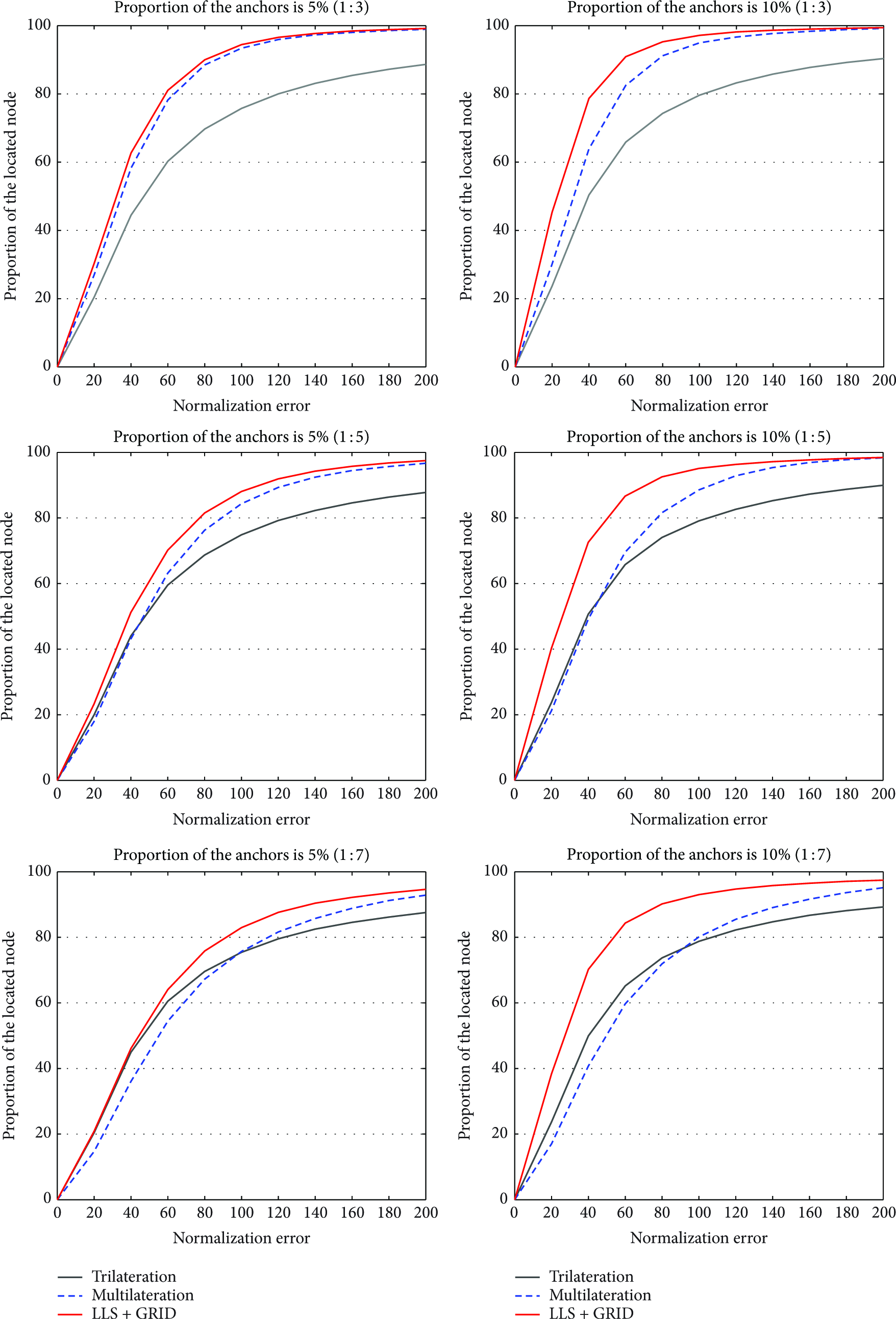
Performance of localization algorithm in nonuniform network.

All the simulation results show that, no matter how heterogeneity of the network is, the LLS-GRID is better than Trilateration and Multilateration. For example, while the percentage of the anchor is 10% and heterogeneity of the network is 1 : 3, for LLS-GRID, the number of the nodes whose location error is less than 40% R is 14.76% more than Multilateration. Similarly, this value is 22.4% and 29.47% more than Multilateration when the heterogeneity degree is 1 : 5 and 1 : 7.

In conclusion, the performance of Multilateration algorithm is unstable with the increase of heterogeneity degree of the network. The same is true for Trilateration. But LLS + GRID algorithm is more stable in these scenes. While the percentage of the anchor is 10% and the heterogeneity degree of the network increases from 1 : 3 and 1 : 7, comparing the number of nodes whose location error is less than 40% R, the location precision of LLS + GRID algorithm only decreases 8.43%, but for Multilateration it is 23.14% decreased. Therefore, we can see LLS + GRID algorithm has more adaptability to the environment.

3.2. Computation

LLS-GRID algorithm only adds a process of choosing anchors before localization, and therefore the amount of calculation of LLS-GRID algorithm and LLS algorithm is similar.

Assume that each unknown node receives n anchor's packet for localization after mask method. We can approximately estimate the amount of calculation based on the times of multiplication and addition in formula (6). $A^T$ is a $2(n-1)$ order matrix and A is $2(n-1)$ order matrix, so $A^{T}A$ need 4 $(n-1)$ times multiplication and $4(n-2)$ times addition. And the result of $A^{T}A$ is a $\mathrm{2}\times \mathrm{2}$ matrix; it needs 16 times multiplication and 8 times addition to calculate the inverse matrix and so on. Based on this, formula (8) needs about $4(n-1)+16+4(n-1)+2(n-1)$ times multiplicity and $4(n-2)+8+2(n-1)+2(n-2)$ times addition. Since most of the hardware can do multiplication or addition only in a single instruction, we consider multiplication and addition as the same calculation; at last, formula (10) needs about 18n times calculation.

Figure 8 illustrates the calculation of LLS-GRID, Trilateration, and Multilateration in different scenarios. From Figure 8, we can see that the calculation of Trilateration is always the smallest in every scene. This is because Trilateration only needs three anchor's packets in localization process. Similarly, the calculation of Multilateration algorithm is always the biggest. This is because Multilateration needs every anchor's packets in localization process. For LLS-GRID algorithm, the calculation is slightly increased than Trilateration but significantly decreased than Multilateration. From Figure 8's result, as the percentage of the anchor is 5% and 10%, the calculation of LLS-GRID is 44% and 72% smaller than Multilateration. So this shows that LLS-GRID algorithm is very stable for every scene, whether in uniform network or nonuniform network. In a word, LLS-GRID algorithm can improve localization accuracy while reducing the calculation cost.

Figure 8

The calculation of localization algorithms.

4. Conclusion

This paper proposes a novel grid-based linear least squares (LLS) self-localization algorithm in WSN. The result of simulation indicates that this algorithm effectively solved the problem of localization precision and computation complexity. This algorithm does not require changing the structure of hardware and the protocol structure. The localization precision of LLS-GRID is vastly superior to Trilateration and Multilateration. Meanwhile, the calculation of the algorithm is only equivalent to 30%~40% of Multilateration. In addition, it is more stable than Multilateration. So this grid-based LLS algorithm can greatly extend the application range of range-free localization method.