An Improved 3D Localization Algorithm for the Wireless Sensor Network

Abstract

Location information is crucial in the wireless sensor network. The nodes in wireless sensor networks are often deployed in the three-dimensional scenario. Therefore, the three-dimensional localization algorithm has become hot in wireless sensor networks. However, existing 3D localization algorithms have shortcomings, such as high complexity, low positioning accuracy, and great energy consumption. Aiming at the existing problems of the current 3D localization algorithms, an improved 3D localization algorithm based on Degree of Coplanarity (3D-IDCP) is proposed. The concept of coplanarity is added into the traditional DV-Distance algorithm to reduce the positioning error caused by anchor nodes which are coplanar. Those unknown nodes which have been located are promoted to assistant anchor nodes to improve the positioning coverage. The simulation results show that the proposed method is accurate in positioning and can enhance the positioning coverage.

1. Introduction

Wireless Sensor Networks (WSNs) are composed of a large number of sensor nodes which can collect, compute, and communicate. The sensor nodes form a multihop and self-configured network by means of wireless communication. Sensor nodes deployed in the monitoring area collect and process the information within the monitoring area and then send the information to the observer [1]. It is important to get the location of the sensor nodes. The information collected without location is always meaningless, so localization becomes a key technology in the Wireless Sensor Network.

Since sensor nodes are randomly deployed in the monitoring area, the manual embedding of location in each node is not feasible in many applications. Nodes often get deployed by aircrafts. Global Positioning System (GPS) receivers can determine their location in the area of deployment, but putting GPS receiver on each node is not feasible due to the increasing cost [2]. Instead, the GPS receiver is only deployed on a small number of sensor nodes and then locates the sensor nodes, which are called anchor nodes. Generally, localization approaches in WSNs locate unknown nodes through the location of anchor nodes.

Currently, localization approaches mainly focus on the 2D plane. Since in practice, the nodes in Wireless Sensor Networks are often deployed in the 3D scenario, for example, deep sea, hill or forest, even sky, and so forth, the localization in a three-dimensional environment is more popular and will lead to further development of localization technology. The three dimensional environment is much more complicated and the computational complexity increases greatly. As a result, it is not appropriate to extend the 2D localization algorithm to a 3D algorithm directly. The research on three-dimensional localization is more realistic and localization algorithms in the three-dimensional space are necessary.

In this paper, an improved 3D localization algorithm and a 3D localization model are proposed to improve positioning accuracy and coverage. The proposal utilizes the range-based localization and includes four phases. The concept of Degree of Coplanarity is added and the best positioning unit based on the Degree of Coplanarity is selected to ensure positioning accuracy. In addition, the unknown nodes which have been located are promoted to assistant anchor nodes. Thus, the positioning coverage is improved with the increasing proportion of anchor nodes. Finally, the performance of the method is verified and compared with other algorithms. The simulation results show that the proposed method outperforms the other two algorithms in terms of positioning accuracy, coverage, and stability.

Following is a summary of the key contributions:

• (i)

The traditional DV-Distance algorithm is modified. The positioning error caused by cumulative distance is reduced through the correction parameter.

(ii)

The best positioning unit based on DCP value is selected to reduce the positioning error caused by coplanar anchor nodes.

(iii)

The idea of promoting unknown nodes to assistant anchor nodes is proposed in order to increase anchor nodes and improve the positioning coverage.

(iv)

Quasi-Newton method is used to correct the position estimated by quadrilateration.

(v)

The simulation shows that 3D-IDCP algorithm is more accurate in positioning and the coverage is higher compared with other 3D localization approaches.

The rest of the paper is organized as follows. The second section introduces the related work of three-dimensional localization algorithms. In Section 3, the three-dimensional localization model is described in details. In Section 4, the process of the algorithm is described. Section 5 is a report of the simulation results and Section 6 is the conclusion and a prospect for further work.

2. Related Work

With the development and application of WSN technology, there is a higher requirement for localization accuracy. At present, research on two-dimensional localizations of the wireless sensor network has become mature, but the study of three-dimensional localizations is still in its infancy.

Zhang et al. present a Landscape-3D space positioning algorithm [3] using mobile assisted. Landscape-3D is the first robust 3D range-based localization algorithm, in which the localization accuracy relies on the expensive mobile beacon. 3D MDS-MAP [4], 3D DVHOP [5], and 3D centroid [6] are range-free localization algorithms modified from 2D plane scenarios directly. These approaches are complex and the localization is not accurate enough.

In recent years, many improvements have been made. Peng and Li propose the DR-MDS algorithm [7], which mainly calibrates the coordinates of nodes and the range of nodes based on the multidimensional scaling. It calculates the distance between any nodes exactly according to the hexahedral measurement and introduces a modification factor to calibrate the distance measured by Received Signal Strength Indicator (RSSI). But the DR-MDS algorithm is complex in calculation. Zhang et al. put forward a hybrid localization approach [8] to overcome the weakness of range-free and range-based algorithms by combining RSSI value and hop distance for 3D WSN localization. The proposed method is more accurate. The algorithm assumes that there is no hole existing in the 3D network. It is not suitable in different irregular 3D network. Feng and Yi propose a decentralized 3D positioning algorithm [9] based on RSSI ranging and free ranging mechanism. Firstly, the algorithm measures the beacon nodes in the neighborhood through RSSI and then obtains initial location information of unknown nodes through regional division. Finally, the method updates the position information through iterative optimization. Iterative optimization can improve the positioning accuracy, but the regional division is easily affected by RSSI measurement error. Chaurasiya et al. propose a novel distance estimation algorithm [2] to estimate the distance between each node and every other node in the network. The proposed algorithm reduces the computational overhead on individual nodes with a centralized approach. The limitation of the algorithm is that it needs a minimum node density to execute the nodes in the localized network successfully.

In order to improve the accuracy of the 3D localization algorithm, localization can be transformed into an optimization problem and the localization result can be optimized with various optimization methods. Intelligent optimization algorithms such as genetic algorithm, least squares support vector machine (SVM) algorithm, and particle swarm optimization algorithm are used in the study of three-dimensional space localization [10–12].

So far, no three-dimensional positioning method has been widely recognized [13]. Existing positioning methods are proposed under certain conditions. The methods need to make choices among factors such as positioning accuracy, computational complexity, node density, communication cost, energy consumption, and positioning coverage. Therefore, it is necessary to conduct a deep research on three-dimensional localization algorithms to design an algorithm with a better and more comprehensive performance.

Compared with two-dimensional localization algorithms, three-dimensional localization algorithms have the following difficulties:

• (1)

More anchor nodes are needed for localization. In a two-dimensional space, it needs at least three anchor nodes, while in a three-dimensional space, it needs at least four anchor nodes to locate the unknown nodes. It not only needs to increase the node density but also makes the algorithm more complex.

(2)

The terrain obstacles will affect the transmission signal. The impact of the obstacles cannot be ignored. There is a certain error in the distances between nodes measured by RSSI, which will affect the positioning accuracy.

In conclusion, there is no fixed standard for three-dimensional localization. There are achievements in 3D localization algorithms, but on the whole, 2D localization algorithm is extended to the 3D space. Currently, there are still many problems in 3D localization algorithms, such as low accuracy, high computational complexity, low positioning coverage and relying too much on anchor nodes. Therefore, further research on localization algorithms for WSN with high accuracy and low complexity is still necessary.

Compared with algorithms in literatures [3–6], our method considers the differences between 2D plane and 3D space, and uses the degree of coplanarity to rule out the unsatisfactory positioning unit and get the best positioning unit. Compared with literatures [2, 7–9], RSSI technology is used and the traditional DV-Distance algorithm is modified. Correction parameter is introduced to modify the cumulative distance. Compared with literatures [10–12], Quasi-Newton method is chosen to optimize the localization result because of its good performance and convenience. In addition, the unknown nodes are promoted to assistant anchor nodes for localization. In this way, the number of anchor nodes is increased and the positioning coverage and positioning accuracy are improved with slight incensement in communication cost and computational complexity.

3. Three-Dimensional Localization Model

3.1. Measurement Model Based on RSSI

The most common way of range-based localization is RSSI (Received Signal Strength Indicator) technology. RSSI technology converts the signal attenuation in the transmission process into the distances between the nodes. Due to the signal attenuation in the transmission process, receiving nodes can estimate the distance between sending nodes according to the received signal strength.

Definition 1.

Assume that $\mathrm{P}\mathrm{L}(d)$ is the signal strength when two sensor nodes are d meters apart.

The wireless signal transmission model is shown as [14]

$$\begin{array}{cc}& \text{PL}\left(d\right)=\text{PL}\left(d_0\right)-10n\text{lg}\left(\frac{d}{d_0}\right)-X_{\sigma },\end{array}$$

(1)

where $d_{\mathrm{0}}$ is const and $\mathrm{P}\mathrm{L}(d_{\mathrm{0}})$ is the signal strength when they are $d_{\mathrm{0}}$ meters apart and it is often got from the experiment experience. n is the wireless channel attenuation coefficient and it is often set around 2~4. $X_{\sigma }$ is the random variable that obeys normal distribution with an expectation of zero and a variance of ${\sigma }^{\mathrm{2}}$ .

In (1), $d_{\mathrm{0}}$ is known, so $\mathrm{P}\mathrm{L}(d_{\mathrm{0}})$ is known as well. Therefore, $\mathrm{10}n\text{lg}(d_{\mathrm{0}})$ is also known. Take $X_{\sigma }$ as a constant value, so RSSI value can be obtained from

$$\begin{array}{l}\text{RSSI}=\text{PL}\left(d\right)\\ =-10n\text{lg}d+\left[10n\text{lg}{d}_0+\text{PL}\left(d_0\right)-X_{\sigma }\right].\end{array}$$

(2)

Equation (2) can be written as (3) because the part in parentheses is constant:

$$\begin{array}{cc}& \text{RSSI}=\text{PL}\left(d\right)=-\mathrm{10}n\text{lg}d+a,\end{array}$$

(3)

where $a=\mathrm{10}n\text{lg}{d}_{\mathrm{0}}+\mathrm{P}\mathrm{L}(d_0)-X\sigma$ and a is a constant value.

Furthermore, the distance d between the sending node and the receiving node can be calculated with

$$\begin{array}{cc}& d=\mathrm{1}{\mathrm{0}}^{\left(a-\text{RSSI}\right)/\mathrm{10}n}.\end{array}$$

(4)

3.2. Modified DV-Distance Mechanism

The DV-Distance localization algorithm [15] is proposed by Niculescu and Nath. It adopts the method similar to the distance vector routing to get the cumulative distance. When each unknown node gets three or more cumulative distances from anchors, the algorithm locates the unknown nodes through trilateration and DV-Distance localization algorithm can be divided into three steps [16].

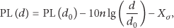
In the first step, each anchor node broadcasts a beacon to be flooded through the network containing the location with node ID and RSSI value. Each receiving node calculates the distance between its adjacent nodes based on the RSSI model above. Then, they will count the cumulative distance or the polyline-distance ${\mathrm{d}\mathrm{i}\mathrm{s}}_{ij}$ from themselves to anchors that they can receive by cumulating the polyline-distance between hop and hop.

In the second step, once an anchor node i gets the polyline-distance to anchor node j, it calculates a correction ratio ${\mathrm{c}\mathrm{o}\mathrm{r}}_{ij}$ of polyline-distance ${\mathrm{d}\mathrm{i}\mathrm{s}}_{ij}$ to straight-line ${\mathrm{D}\mathrm{i}\mathrm{s}}_{ij}$ between the two anchors i and j, which is then flooded to the entire network as the network correction. When an unknown node k accepts the information from one anchor node j, it uses the polyline-distance ${\mathrm{d}\mathrm{i}\mathrm{s}}_{kj}$ from anchor nodes to compute the amended distance ${\mathrm{D}\mathrm{i}\mathrm{s}\mathrm{C}\mathrm{o}\mathrm{r}\mathrm{r}}_{kj}$ between itself and the anchor nodes.

In the last step, when the unknown nodes get three or more distances from anchor nodes, their location is calculated through trilateration or maximum likelihood estimation.

The modified DV-Distance Mechanism is improved in two respects.

(i) In DV-Distance algorithm, the error will be larger if the actual distance is replaced by the cumulative distance when there are more hops between them, so the cumulative distance must be modified.

Definition 2.

Assume i is the ID of node, $i=1,2\cdots n$ . $L_{ij}$ is the actual distance between anchor node i and anchor node j. $D_{ij}$ is the cumulative distance between node i and anchor node j. Assume that the unknown node receives location information from n anchor nodes; then, the correction parameter ${\lambda }_k$ of the unknown node K and the anchor node i can be calculated with

$$\begin{array}{cc}& {\lambda }_k=\frac{\sum L_{ij}}{\sum D_{ij}}.\end{array}$$

(5)

If the cumulative distance between anchor node i and the unknown node K is $D_{ki}$ , the corrected cumulative distance can be obtained with

$$\begin{array}{cc}& L_{ki}={\lambda }_{ki}\ast D_{ki}.\end{array}$$

(6)

Regard the corrected cumulative distance as the effective distance between the unknown node K and the anchor node i, and then locate the unknown node K. It can reduce the positioning error.

(ii) In the last step, when extended to the 3D space, the unknown nodes must get four or more distances from anchor nodes.

3.3. Anchor Selection Based on Coplanarity

After getting the distances between unknown nodes and anchor nodes, we can estimate the location of unknown nodes through the distances and location of anchor nodes.

In the process of positioning, the combination of anchor nodes which can determine an unknown node through multilateral localization is called a positioning unit. In the two-dimensional plane, a positioning unit consists of at least three anchor nodes. When calculating the location of the unknown node through trilateration, it is impossible to locate the unknown node when the three anchor nodes are in a straight line. The same problem also exists in the three-dimensional space. A positioning unit in the three-dimensional space requires at least four anchor nodes. Due to the error of RSSI measurement, four spherical surfaces do not necessarily have an intersection point. In addition, it is hard to locate the unknown node when the four anchor nodes are almost coplanar. In order to solve this problem, degree of coplanarity is introduced [17].

Definition 3.

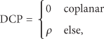
Degree of Coplanarity (DCP) represents the coplanar degree of four anchor nodes in the three-dimensional space.

Definition 4.

In the three-dimensional space, the radius ratio of a tetrahedron is defined as $\rho =\mathrm{3}{r}_{\mathrm{i}\mathrm{n}}/r_{\mathrm{o}\mathrm{u}\mathrm{t}}$ [18].

Where $r_{\mathrm{i}\mathrm{n}}$ and $r_{\mathrm{o}\mathrm{u}\mathrm{t}}$ , respectively, represent the radius of the inscribed sphere and the circumscribed sphere of the tetrahedron.

The radius of the inscribed sphere and the circumscribed sphere of the tetrahedron can be calculated with [18]

$$\begin{array}{cc}& r_{\mathrm{i}\mathrm{n}}=\frac{\mathrm{3}v}{{\sum }_{i=\mathrm{0}}^{\mathrm{3}}{s}_i},\\ r_{\mathrm{o}\mathrm{u}\mathrm{t}}=\frac{\sqrt{\left(a+b+c\right)\left(a+b-c\right)\left(a+c-b\right)\left(b+c-a\right)}}{24v},\end{array}$$

(7)

where v is the volume of the tetrahedron and $s_i$ is the area of the four surfaces. a, b, and c are three products of the edges of the tetrahedron. The radius ratio can be obtained with

$$\begin{array}{l}\rho \\ =\frac{216v^2}{{\sum }_{i=0}^3{s}_i\sqrt{\left(a+b+c\right)\left(a+b-c\right)\left(a+c-b\right)\left(b+c-a\right)}},\end{array}$$

(8)

where $\rho \in (\mathrm{0,1}]$ . When ρ approaches 0, it means the four points are approximating coplanar. When ρ approaches 1, it means the four points form a regular tetrahedron.

Degree of Coplanarity (DCP) can be expressed with

$$\begin{array}{cc}& \text{DCP}=\left\{\begin{array}{cc}\mathrm{0}\hfill & \text{coplanar}\hfill \\ \rho \hfill & \text{else,}\hfill \end{array}\right.\end{array}$$

(9)

where $\mathrm{D}\mathrm{C}\mathrm{P}\in (\mathrm{0,1}]$ .

Definition 5.

The positioning unit with maximum DCP value is called the best positioning unit.

The DCP value ensures that the best positioning unit can be selected. With the DCP value, anchor nodes which are coplanar can be ruled out so that positioning accuracy will be improved. Meanwhile, it will decrease the proportion of positioning units, so there is no positioning unit for some unknown nodes to locate themselves. In order to solve this problem, the idea of assistant anchor nodes is proposed in our scheme.

3.4. Node Localization Model

The localization mode is shown in Figure 1. It needs at least four anchor nodes to determine the location of unknown nodes. From the analysis above, it can be seen that four anchor nodes should not be in the same plane in order to ensure the localization.

Figure 1

Localization model in three-dimensional space.

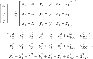
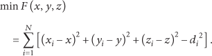
Assume that A, B, C, and D are the four anchor nodes in the positioning unit and their coordinates are known as $(x_1,y_1,z_1)$ , $(x_2,y_2,z_2)$ , $(x_3,y_3,z_3)$ , and $(x_4,y_4,z_4)$ . K is an unknown node with the coordinate $(x,y,z)$ . The distances between anchor nodes and unknown node are $d_{KA}$ , $d_{KB}$ , $d_{KC}$ , and $d_{KD}$ . Equation (10) is obtained according to the distance between the nodes:

$$\begin{array}{cc}& \sqrt{{\left(x_1-x\right)}^2+{\left(y_1-y\right)}^2+{\left(z_1-z\right)}^2}-d_{KA}=0,\\ \sqrt{{\left(x_2-x\right)}^2+{\left(y_2-y\right)}^2+{\left(z_2-z\right)}^2}-d_{KB}=0,\\ \sqrt{{\left(x_3-x\right)}^2+{\left(y_3-y\right)}^2+{\left(z_3-z\right)}^2}-d_{KC}=0,\\ \sqrt{{\left(x_4-x\right)}^2+{\left(y_4-y\right)}^2+{\left(z_4-z\right)}^2}-d_{KD}=0.\end{array}$$

(10)

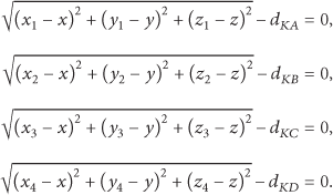
Solve (10) and then get the coordinate of the unknown node K as

$$\begin{array}{l}\left[\begin{array}{l}x\\ y\\ z\end{array}\right]=\frac{1}{2}{\left[\begin{array}{lll}{x}_2-x_1& y_2-y_1& z_2-z_1\\ x_3-x_1& y_3-y_1& z_3-z_1\\ x_4-x_1& y_4-y_1& z_4-z_1\end{array}\right]}^{-1}\\ ·\left[\begin{array}{l}{x}_2^2-x_1^2+y_2^2-y_1^2+z_2^2-z_1^2+d_{KA}^2-d_{KB}^2\\ x_3^2-x_1^2+y_3^2-y_1^2+z_3^2-z_1^2+d_{KA}^2-d_{KC}^2\\ x_4^2-x_1^2+y_4^2-y_1^2+z_4^2-z_1^2+d_{KA}^2-d_{KD}^2\end{array}\right].\end{array}$$

(11)

So far the position of the unknown node K is obtained through quadrilateration.

4. 3D-IDCP Algorithm Description

4.1. Promotion of Assistant Nodes

Generally speaking, anchor nodes are deployed with their locations known. Due to the high cost, the number of anchor nodes is usually limited. Because of the limit of DCP value, some unknown nodes cannot find a proper positioning unit to locate themselves, which lowers the positioning coverage. In order to improve the coverage, the idea of assistant anchor nodes is proposed. The unknown nodes that have located themselves are promoted to assistant anchor nodes can work as anchor node, which will increase the number of anchor nodes and may improve the positioning coverage and accuracy. The steps of promoting unknown nodes to assistant anchor nodes are as follows.

Step 1.

In the first round of localization, choose the best positioning unit based on the DCP value to locate the unknown nodes.

Step 2.

Promote the unknown nodes which have been located to assistant anchor nodes and broadcast their locations. Regard them as anchor nodes in the second round of localization.

Step 3.

Locate those unknown nodes again which fail to be located with both anchor nodes and assistant nodes.

4.2. Model Optimization Based on Quasi-Newton Method

Localization is essentially an optimization problem based on different distances. There is an error in localization algorithms using quadrilateration. In the last stage of localization, Quasi-Newton method can optimize the positioning result.

The Quasi-Newton method [19] is one of the most effective ways for nonlinear optimization. It is often used for unconstrained optimization [20–23]. Quasi-Newton method is selected in the optimization phase of our algorithm because of its good performance in optimization.

Assume that $i=\mathrm{1,2},\dots ,N$ is the ID of the anchor node. The coordinates of anchor nodes are known as $(x_1,y_1,z_1)$ , $(x_2,y_2,z_2)$ , $(x_3,y_3,z_3)$ , and $(x_4,y_4,z_4)$ . The distance between anchor node i and unknown node k is $d_i$ . So the localization can be transformed into an unconstrained optimization problem. Equation (12) is the objective function of the unconstrained optimization problem:

$$\begin{array}{l}\text{min}F\left(x,y,z\right)\\ ={\displaystyle \sum }_{i=\mathrm{1}}^N\left[{\left(x_i-x\right)}^2+{\left(y_i-y\right)}^2+{\left(z_i-z\right)}^2-{d_i}^2\right].\end{array}$$

(12)

Then use Quasi-Newton method for iterative computation, the process of which is shown as follows.

Step 1.

Use the estimated location as the initial value. Calculate $g_{\mathrm{0}}$ with the given initial matrix $H_{\mathrm{0}}$ and control error ε. Set $k=\mathrm{0}$ .

Step 2.

Let $p_k=-H_k{g}_k$ .

Step 3.

Determine the search step length ${\alpha }_k$ with

$$\begin{array}{cc}& f\left(x_k+{\alpha }_k{p}_k\right)=\text{min}f\left(x_k+\alpha p_k\right).\end{array}$$

(13)

Step 4.

Calculate $x_{k+\mathrm{1}}=x_k-{\alpha }_k{H}_k^{-\mathrm{1}}{g}_k$ and $g_{k+\mathrm{1}}=\nabla f(x_{k+\mathrm{1}})$ . If $‖g_{k+\mathrm{1}}‖\le \epsilon$ , the result of the iterative calculation has met the requirement of control error. So stop the iterative calculation and output the result $x^{\ast }=x_{k+\mathrm{1}}$ ; otherwise, go on with the next step.

Step 5.

Set $s_k=x_{k+\mathrm{1}}-x_k$ , $y_k=g_{k+\mathrm{1}}-g_k$ . Calculate $w_k$ with

$$\begin{array}{cc}& w_k={\left(y_k^T{H}_k{y}_k\right)}^{1/2}\left(\frac{s_k}{y_k^T{s}_k}-\frac{H_k{y}_k}{y_k^T{H}_k{y}_k}\right).\end{array}$$

(14)

Step 6.

Calculate $H_{k+\mathrm{1}}^{\%}$ with (15). Let $H_{k+\mathrm{1}}=H_{k+\mathrm{1}}^{\%}$ , $k=k+\mathrm{1}$ . Go to Step 2:

$$\begin{array}{cc}& H_{k+1}^{\%}=H_k-E_k=H_k-\frac{H_k{y}_k{y}_k^T{H}_k}{y_k^T{H}_k{y}_k}+\frac{s_k{s}_k^T}{y_k^T{s}_k}+w_k{w}_k^T.\end{array}$$

(15)

4.3. Algorithm Description

According to the three-dimensional localization model above, the improved scheme mainly consists of four phases. In the first stage, measure the distances between neighbor nodes through RSSI technology. Then, get all the distances between unknown nodes and anchor nodes with the modified DV-Distance algorithm. In the second stage, select the best four anchor nodes as a positioning unit based on the degree of coplanarity. Estimate the location of unknown nodes through quadrilateration. In the third stage, carry out iterative calculation with Quasi-Newton method to optimize the position result. In the last stage, promote those unknown nodes which have been located to assistant anchor nodes. Locate the unknown nodes again which have not been located with the anchor nodes and the assistant anchor nodes.

The process of 3D-IDCP algorithm is shown in Figure 2.

Figure 2

The process of the 3D-IDCP algorithm.

Step 1.

Measure the distance between neighbor nodes with RSSI technology.

Step 2.

Each node in the network receives and forwards the information of the anchor nodes through the distance vector protocol.

Step 3.

Each node checks whether the packet is from the same anchor node. If the node has not received the packet yet, save the packet; otherwise, compare the hop value and save the smaller one.

Step 4.

Check if the broadcast is over. If not, turn to Step 1; otherwise, go on with the next step.

Step 5.

Calculate the cumulative distance between anchor nodes and unknown nodes.

Step 6.

Correct the cumulative distance.

Step 7.

Work out the DCP value of each positioning unit, and choose the best positioning unit based on the DCP value.

Step 8.

Estimate the location of unknown nodes with the positioning unit according to (11).

Step 9.

Transform localization into an unconstrained optimization problem. Optimize the localization result with the Quasi-Newton method. Set the estimated location in Step 7 as an initial value of the Quasi-Newton method and carry out iterative calculation with (14) and (15) until it works out the result that can meet the requirement of control error.

Step 10.

Promote the unknown nodes which have been located to assistant anchor nodes and they can work with anchor nodes in location.

Step 11.

Carry out node localization for the second round with both anchor nodes and assistant anchor nodes to improve the positioning coverage.

5. Simulation Results

In order to verify the performance of the proposed 3D-IDCP algorithm, simulation experiment is carried out with MATLAB 2009a. The environment of the simulation is set as follows. Firstly, all the sensor nodes are randomly deployed in the three-dimensional area of 100 m × 100 m × 100 m. Secondly, the communication radius R is set 40 meters. Experiments are carried out 50 times. Each time sensor nodes are randomly deployed.

In the simulation, RSSI is simulated through the $\mathrm{r}\mathrm{s}\mathrm{s}\mathrm{i}(d,a)$ function in rssi.m file. In this function, DOI propagation model is selected to get the RSSI value. In $\mathrm{r}\mathrm{s}\mathrm{s}\mathrm{i}(d,a)$ function, d represents the actual distance between two nodes which can be easily got in the deployment part and a is a parameter that changes with the environment. Set $d_0=20$  m in (1) and $a=7$ . The estimated distance can be obtained with the RSSI value.

The localization accuracy, positioning coverage, and stability of the algorithm are, respectively, evaluated by LER (Localization Error Ratio), LNP (Localized Node Proportion), and BNP (Bad Node Proportion). Bad anchor nodes refer to unknown nodes with a localization error bigger than their communication radius R:

$$\begin{array}{cc}& \text{Localization Error}={\displaystyle \sum }_{i=\mathrm{1}}^n\sqrt{{\left(x_n-x_n^{\prime }\right)}^{\mathrm{2}}+{\left(y_n-y_n^{\prime }\right)}^{\mathrm{2}}},\\ \text{LER}=\frac{{\sum }_{i=\mathrm{1}}^n\sqrt{{\left(x_n-x_n^{\prime }\right)}^{\mathrm{2}}+{\left(y_n-y_n^{\prime }\right)}^{\mathrm{2}}}}{n\times R},\\ \text{LNP}=\frac{n_{\text{localized}}}{n},\\ \text{BNP}=\frac{n_{\text{bad}}}{n_{\text{localized}}},\end{array}$$

(16)

where n is the number of unknown nodes, $(x_n,y_n)$ is the actual location of unknown nodes, and $(x_n^{\prime },y_n^{\prime })$ is the calculated location of unknown nodes. R is the radio range of sensor nodes. $n_{\mathrm{l}\mathrm{o}\mathrm{c}\mathrm{a}\mathrm{l}\mathrm{i}\mathrm{z}\mathrm{e}\mathrm{d}}$ is the number of unknown nodes successfully located. $n_{\mathrm{b}\mathrm{a}\mathrm{d}}$ is the number of bad nodes.

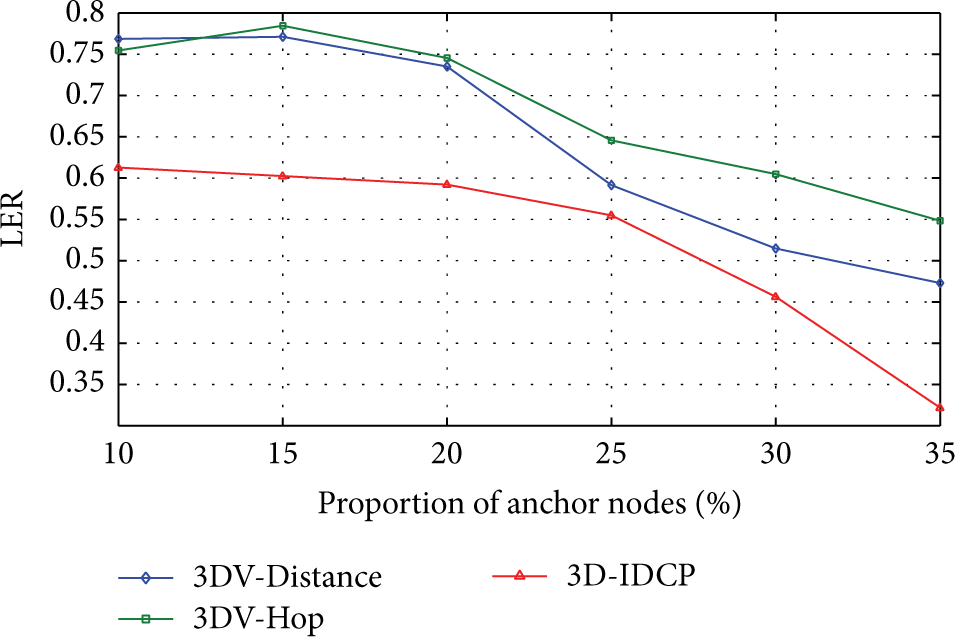
In the simulation experiment, the 3D-IDCP algorithm is compared with another two algorithms, namely, 3DV-Distance algorithm and 3DV-Hop algorithm. 3DV-Distance algorithm is the extension of DV-Distance [15] algorithm in the 3D space. 3DV-Hop algorithm is the extension of DV-Hop [24] algorithm in the 3D space. Both algorithms extend the 2D localization algorithm to into 3D directly. Compared with them, this scheme adds correction parameter to modify the distance between anchor nodes and unknown nodes and uses DCP value to select the positioning unit.

Figure 3 shows the effect of the 3D-IDCP algorithm. The green circle represents anchor nodes deployed in the three-dimensional space. The red triangle represents the unknown nodes. The red cross represents the calculated location of the unknown nodes.

Figure 3

The effect of the 3D-IDCP algorithm.

Figure 4 shows the Localization Error Ratio (LER) of three kinds of 3D localization algorithms. Experiments are carried out 50 times. Each time sensor nodes are randomly and differently deployed. According to the average value, the 3D-IDCP algorithm performs better than the 3DV-Distance algorithm and 3DV-Hop algorithm in terms of Localization Error Ratio. Reduce the LER to 16% and compare it with 3DV-Distance algorithm and 22% compared with 3DV-Hop algorithm. The positioning accuracy improves with more anchor nodes deployed in the space.

Figure 4

Comparison in LER.

The connectivity level of a network will affect localization too. Observe the changes of LNP and BNP when the connectivity of the network is different.

Figure 5 shows the LNP of three kinds of 3D localization algorithms. The 3D-IDCP algorithm performs better than the other two algorithms. In our scheme, when the network connectivity comes up to 10, the positioning coverage reaches 1, which means all the unknown nodes can be located successfully. Our scheme improves the positioning coverage up to 21% and 25%, respectively, compared with 3DV-Distance algorithm and 3DV-Hop algorithm.

Figure 5

Comparison in LNP.

Figure 6 shows the BNP of three kinds of 3D localization algorithms. There are fewer bad nodes in 3D-lDCP compared with the other two algorithms. In our scheme, when the network connectivity comes up to 10, there is no bad node in the localization. Our scheme is more stable than the other two algorithms.

Figure 6

Comparison in BNP.

It can be seen from Figures 4–6 that our algorithm outperforms the other two algorithms in positioning accuracy, positioning, and stability.

6. Conclusion and Future Work

Aiming at the low accuracy of three-dimensional localization algorithms, an improved three-dimensional localization algorithm is proposed. Base on the traditional DV-Distance, the degree of coplanarity is introduced and Quasi-Newton method is used to optimize the positioning result. The simulation experiments have verified the effect of the proposed algorithm in positioning accuracy, positioning coverage, and proportion of bad nodes. The future work will be concentrated on the application of the actual WSN environment.