Communication Availability-Based Scheduling for Fair Data Collection with Path-Constrained Mobile Sink in Wireless Sensor Networks

Abstract

To effectively transfer sensing data to a sink node, system designers should consider the characteristic of wireless sensor networks in the way of data transmission. In particular, sensor nodes surrounding a fixed sink node have routinely suffered from concentrated network traffic so that their battery energy is rapidly exhausted. The lifetime of wireless sensor networks decreases due to the rapid power consumption of these sensor nodes. To address the problem, a mobile sink model has recently been chosen for traffic load distribution among sensor nodes. However, since a mobile sink continuously changes its location in sensor networks, it has a time limitation to communicate with each sensor node and unstable signal strength from each sensor node. Therefore, fair and stable data collection policy between a mobile sink and sensor nodes is necessary in this circumstance. In this paper, we propose a new scheduling policy to support fair and stable data collection for a mobile sink in wireless sensor networks. The proposed policy performs data collection scheduling based on the communication availability of data transmission between sensor nodes and a mobile sink.

1. Introduction

Wireless sensor networks have been exploited in many application fields, such as wild habitats monitoring and military purposes [1–3]. In wireless sensor networks, sensor nodes relay sensing data to a sink node. The sink node can evaluate sensing data and also transmit it to external networks to notify applied field states. To relay the sensing data, sensor nodes work on multiple hops.

Existing wireless sensor networks frequently use the fixed sink node model owing to the simplicity of sensor deployment [4, 5]. In the configuration of a wireless sensor network with a fixed sink node, the sensor nodes near the sink node should perform relay operations for many data packets transmitted from neighboring sensor nodes. This characteristic of the fixed sink node causes a rapid drain on the batteries of the sink node's surrounding sensor nodes. When the power of these sensor nodes drains completely, sensing data from the terminal sensor nodes cannot be transferred to the sink node. This results in a major source of shortened lifespan for total wireless sensor networks.

To address the problem of the fixed sink node, a mobile sink model was introduced to distribute battery energy consumed by relaying sensing data into all sensor nodes. According to [6–8], the mobile sink model provides better throughput scaling and increased network lifetime. In [9], a routing protocol named MSRP is suggested to prolong the network lifetime in clustered wireless sensor networks. In addition, the authors in [10] showed the energy efficiency of the mobile sink model compared to static sink model.

In our mobile sink model, we consider the public transport vehicles such as buses or trains, which make it more realistic than random mobility models. Generally the public transport vehicles periodically move on the constrained path. In this scenario, air pollution or traffic information can be fascinating information to be collected.

Basically the mobile sink moves across the deployed sensor nodes and receives the data packets from only those sensor nodes that are within the communication range of the mobile sink. Since the communication range is limited, each sensor node has limited time for data transmission. In this condition, the mobile sink should evenly collect data from all sensor nodes. If the mobile sink cannot receive sensing data from any of the sensor nodes, the location-monitoring information cannot be grasped completely by these sensor nodes. Thus, the ultimate object of deployed wireless sensor networks also fails. Addressing the problem requires data collection scheduling policies for the mobile sink.

The staying time of sensor nodes within the communication range of a mobile sink does affect the data collection process. The available communication time of each sensor node is different according to their deployed locations. In addition, since the mobile sink moves continuously, the communication errors between sensor nodes and a mobile sink vary every moment. The remote sensor nodes from a mobile sink suffer from high communication errors and have short staying time. For them, when the mobile sink performs data collection scheduling, it allocates high priority order and a long data communication period. Otherwise, for the sensor nodes having low communication errors and relatively long staying time, the mobile sink assigns short communication time for data transmission.

This paper proposes a new data collection scheduling policy based on the dynamic working environment of a mobile sink. The aim of the proposed policy supports fair data collection between all deployed sensor nodes within the communication range of a mobile sink. Deciding the priority order of sensor nodes, it reflects the communication error rates of sensor nodes that are varied according to the distance to a mobile sink. In addition, the proposed policy uses the amount of received data from each sensor node as the weight of data collection scheduling. Based on these scheduling criteria, the proposed policy dynamically controls communication time for all sensor nodes. Thus, it provides fair data collection for a mobile sink in wireless sensor networks.

The remainder of this paper is organized as follows. In the next section, we review the background to a mobile sink and scheduling policies in wireless sensor networks. In Section 3, we describe the detailed motivations of fair data collection, and in Section 4, we introduce a new scheduling policy to support fair data collection in the mobile sink. Section 5 offers measurement and evaluation of the performances of scheduling policies. Finally, our conclusions and ideas for future work regarding this research are given in Section 6.

2. Related Work

2.1. Mobile Sink

Several studies have explored the mobile sink in wireless sensor networks in routing topology, and they have analyzed the transferring of sensing data and the movement controlling of mobile sinks [11, 12]. The routing technologies derived from the fixed sink model cannot be applied to the mobile sink model. Since the mobile sink moves constantly, the routing path to transfer the sensing data varies. To support this environment, the routing table must be changed frequently according to the location of mobile sinks. The constant change of the routing table burdens the sensor nodes with a heavy workload, which causes a rapid battery drain on the sensor nodes. The movement control of the mobile sink represents an important research topic for the effective use of wireless sensor networks. If the speed and movement of mobile sinks can be controlled, data collection could be adjusted according to the state of each sensor node. For example, when each sensor node generates different amounts of sensing data, the mobile sink stays longer in the areas that have potential for sensing data. This approach offers effective data collection opportunities for the mobile sink.

The path-constrained mobile sink has been studied as well [13–15]. The queuing theory has been applied to data collection areas of a mobile sink [13]. This research introduced queuing models to analyze the sensor nodes located in the communication range of a mobile sink. Based on defined queuing models, this method monitored the range of RF antenna strength of sensor nodes, which allow the mobile sink to receive all sensing data. In [14, 15], the authors proposed the algorithm for fair data collection with a mobile sink. However, the algorithm randomly selects a sensor node to collect data and only the amount of sensing data is considered to calculate the data transmission time.

However, those researches focused on the receipt of all data perceived by individual sensor node. If sensor nodes deviate from the communication range of the mobile sink before the complete transmission of all data, loss of the remaining data is assumed. This characteristic causes a mobile sink to miss parts of the sensing data. In addition, it wastes the computing resources of sensor nodes for monitoring the field area and for relaying neighboring sensor node data. To solve this problem, the proposed method performs a fair data collection scheduling policy for all sensor nodes.

2.2. Scheduling Policies

Many studies have looked at scheduling policies to provide fairness of transmission opportunity for network users. The Generalized Processor Sharing (GPS) algorithm transmits data packets to users in a round-robin style [16, 17]. This algorithm achieves ideological fairness by dividing packets and transmitting them to queues. However, implementation of this idea has many difficult problems. To compensate for these problems, the Weighted Fair Queuing (WFQ) algorithm was proposed [18]. It was known as the Packet-by-Packet GPS (PGPS) model. In this algorithm, all data packet queues have their priority and the queue with the highest priority receives preferential service. This approach is usually adapted to support fairness in data processing for multiple queues. An optimal packet-based approximation of GPS is given by Worst-case Fair Weighted Fair Queuing (WF²Q) that provides almost identical service to GPS with a maximum difference of one packet size [19].

Besides applying the queuing policies to scheduling algorithms, the round-robin policy was frequently adapted as the representative scheduling algorithm [20]. The Packet-Based Round Robin (PBRR) algorithm schedules the data packets of multiple queues in a round-robin style, one by one. The implementation of this algorithm is easy, but its fairness property applies only to same-size packets. It cannot guarantee fairness to varied size packets in data processing for multiple queues. The PBRR can be extended to Weighted Round Robin (WRR) which is the simplest approximation of GPS [21]. To handle packets of variable size without knowing their mean size, Deficit Weighted Round Robin (DWRR) was proposed [22].

3. Mobile Sink Characteristics

3.1. Deployment

Figure 1 shows the deployment of wireless sensor networks composed of N sensor nodes. These sensor nodes are distributed randomly and work independently at their fixed locations. Each sensor node can transmit sensing data to a mobile sink within single hops. The mobile sink communicates with the sensor nodes located in the communication range of a single hop from its moving path. The mobile sink continuously moves in the path through randomly distributed sensor nodes and does not change its course.

Figure 1

Mobile sink and wireless sensor nodes.

3.2. Limited Communication Time

The available communication time for sensor nodes is limited according to the movement of the mobile sink. Figure 2 shows the communication range when a mobile sink makes contact with sensor nodes A and B. The mobile sink moves from left to right and the dotted line circle represents the communication range of the mobile sink. Sensor nodes A and B can communicate with the mobile sink from their entering point IN to deviating point OUT. In other positions, they cannot communicate with the mobile sink because they have moved out of the communication range. Thus, each sensor node has its specific time zone for communicating with a mobile sink. For this period, sensor nodes should communicate with a mobile sink. Due to communication errors, missing information could cause serious problems in specific application fields dependent on wireless sensor networks.

Figure 2

Path of the mobile sink and sensor nodes.

The limited communication time varies according to both the moving path of the mobile sink and the distances to sensor nodes. As the sensor node is far away from the mobile sink's moving path, it has short communication time. In Figure 2, the sensor node A is located far away as compared to sensor node B so it has shorter communication time.

3.3. Communication Error Variation

The communication error rate varies according to the distance between a mobile sink and sensor nodes. To consider those, we use shadowing model in radio propagations. The shadowing model is comprised of two models. Firstly, it is the path loss model in which the received power is predicted by the distance d. The received power can be derived from the reference distance $d_0$ and the path loss exponent β as follows [23, 24]:

$$\begin{array}{cc}& \frac{P_r\left(d_{\mathrm{0}}\right)}{\stackrel{-}{P_r\left(d\right)}}={\left(\frac{d}{d_{\mathrm{0}}}\right)}^{\beta }.\end{array}$$

(1)

The $P_r(d_0)$ means the received power at reference distance $d_0$ in free space. The second part of shadowing model is to apply the log-normal random variable which represents the variation of the received power at distance d. The log-normal random variable follows the Gaussian distribution so consequentially the shadowing model is made by

$$\begin{array}{cc}& \left[\frac{P_r\left(d\right)}{P_r\left(d_{\mathrm{0}}\right)}\right]=-\mathrm{10}\beta \log \left(\frac{d}{d_{\mathrm{0}}}\right)+X_{dB},\end{array}$$

(2)

where the $X_{dB}$ is the Gaussian random variable called shadowing deviation.

The signal strength by the distance and the packet reception rate by the Signal-to-Noise Rate (SNR) are represented as shown in Figure 3. Also, the packet reception rate and packet error rate by the distance between sensor nodes can be calculated as shown in Figure 4. These three graphs are based on the shadowing model explained above. We used 2 for path loss exponent β, 4 for shadowing deviation $X_{dB}$ , and 1 for the reference distance $d_0$ [25]. As shown in Figure 3, the signal strength is rapidly reduced as the distance increases, while the packet reception rate rapidly reduced as the SNR decreases. In Figure 4, the packet reception rate decreases as the distance increases. It shows that the pattern of the packet reception rate and the packet error rate in Figure 4 is based on the signal strength variation represented in Figure 3.

Figure 3

Signal strength by distance and packet reception rate by SNR.

Figure 4

Packet error and packet reception rate by the distance.

Figure 5 denotes the packet reception rate for the two sensor nodes A and B of Figure 2. As shown in Figure 5(a), the sensor nodes A and B have the longest communication distance at the point IN. The communication distance is continuously reduced as the mobile sink moves. Due to the movement of the mobile sink, the communication distance increases again. Consequentially at point OUT, the communication distance becomes the same distance with the distance at point IN. Since the packet reception rate is reduced by the increase of the communication distance, the packet reception rate for the mobile sink will be deployed as shown in Figure 5(b).

Figure 5

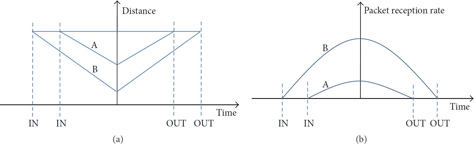
The variation of packet reception rate.

3.4. Needs for Fair Data Collection

In wireless sensor networks, sensor nodes can be disseminated uniformly or they can spread randomly. To receive sensing data from sensor nodes, a mobile sink moves in the working area of the deployed sensor networks. The mobile sink preserves an available communication range according to its RF capability. As the mobile sink moves, some sensor nodes can connect with, and other sensor nodes can deviate from, the communication range of the mobile sink. Thus, the sensor nodes have a limited communication time after entering the communication range and undergoing the variation of communication errors. These characteristics directly affect the packet reception rates of a mobile sink.

If a mobile sink does not have enough time to receive total data from all sensor nodes (it can occur because the public transport vehicles are controlled by passengers not by the purpose of the data collection), it has to collect a fair amount of data from all sensor nodes within limited communication time. For example, when ten sensor nodes are deployed, only if five sensor nodes transmit 100% of total sensing data and other sensor nodes transmit 0%, the information achieved from wireless sensor networks can be restricted and distorted. Additionally, if the sensor nodes cannot transmit data repetitively, the buffer of the sensor nodes will overflow because generally the buffer capacity of sensor nodes is very low due to the small size and the battery driven operation of sensor nodes. To address this problem, a mobile sink should perform a fair data collection scheduling policy on the sensor nodes that have entered the communication area of the mobile sink. To support fair data reception from all sensor nodes, the mobile sink should consider both the limited communication time and communication error variations.

4. Communication Availability-Based Scheduling for Fair Data Collection (CASF)

This paper proposes Communication Availability-based Scheduling for Fair Data Collection (CASF) in wireless sensor networks. CASF provides a fair opportunity to each sensor node. It adapts data collection scheduling to limited communication time and communication availability, which are mobile sink's characteristics.

To design CASF, the deployment of sensor nodes was first investigated. CASF is composed of a priority assignment process and communication time allocation process. The priority assignment process selects a sensor node among all sensor nodes within a given mobile sink communication range. The selected senor node takes communication time allocation from a mobile sink and transmits the data to the mobile sink during this time.

4.1. Investigation of the Sensor Nodes

Before receiving data from sensor nodes, the mobile sink examines the distribution of sensor nodes to calculate their staying time in a mobile sink communication range. The mobile sink periodically sends the beacon messages to the sensor nodes to estimate their communication time. Figure 6 shows the moving route of the mobile sink, periodically broadcasting beacon messages onto the sensor nodes. $T_{\mathrm{i}\mathrm{n}}$ represents the entrance time of a sensor node, and $T_{\mathrm{o}\mathrm{u}\mathrm{t}}$ represents its departure time. For the process of moving, if a sensor node approaches the communication range of the mobile sink, the sensor node sends an ACK message to the mobile sink. Based on this ACK message, the mobile sink can find the $T_{\mathrm{i}\mathrm{n}}$ time of the corresponding sensor node. In addition, if the sensor node no longer sends an ACK message, the mobile sink regards it as moving out from the communication range. Therefore, $T_{\mathrm{o}\mathrm{u}\mathrm{t}}$ is estimated in the mobile sink. Based on the difference between $T_{\mathrm{i}\mathrm{n}}$ and $T_{\mathrm{o}\mathrm{u}\mathrm{t}}$ , the mobile sink calculates the communication period of sensor nodes in the communication range.

Figure 6

Entrance/departure of communication range.

4.2. Priority Order for Sensor Nodes

After investigating the distribution of sensor nodes in wireless sensor networks, a mobile sink moves to receive data. During a moving period, a mobile sink can make contact with sensor nodes more than one sensor node. Among them, a mobile sink has to decide upon priority orders for data collection scheduling and select one sensor node to receive data. When deciding priority orders, a mobile sink should support fair data transmission opportunities for all sensor nodes within a communication range. For this, CASF uses following equation to decide the priority orders of sensor nodes:

$$\begin{array}{cc}& \mathrm{P}=\mathrm{R}\mathrm{R}\times \mathrm{R}\mathrm{D},\end{array}$$

(3)

•  

  P: priority order,

•  

  RR: ${\int }_{\mathrm{c}\mathrm{r}}^{\mathrm{o}\mathrm{u}\mathrm{t}}(P_r\left(d_0\right)\times (-10\beta \log \left(d_t/d_0\right)+X_{dB}))\hspace{0.17em}dt$ , reception rate,

•  

  RD: amount of received data.

Equation (3) is composed of an RR item and RD item. The RR is the packet reception rate and is used to select the sensor node that has the least availability in the aspect of data transmission opportunity. The cr in the RR is the start time and the out is the corresponding sensor node's deviation time from the communication range of a mobile sink. As explained in Section 3, since the packet reception rate is related to signal strength, we used the shadowing model for calculating the RR. Therefore, the total amount of packet reception rates between a mobile sink and a sensor node can be represented as the integral of the inverse parabola from the starting time to the deviation time. The sensor node with the least integral value has the highest probability in a data transmission opportunity. As sensor nodes move away from a mobile sink, the availability of data transmission is reduced due to the communication errors. The RR reflects this characteristic in (3).

The RD is the accumulated amount of data packets transmitted by a sensor node. The RD reflects previously transmitted packets when deciding the priority order. It grants high priority to the sensor node with less data transmission history. Finally, (3) selects one sensor node among sensor nodes within a mobile sink communication range. The selected sensor node has the least availability in data transmission opportunity and the least amount of data transmissions. It is a principle of CASF to support fair data collection scheduling in a mobile sink.

Figure 7 shows an experimental platform of wireless sensor networks with a mobile sink and four sensor nodes. The mobile sink successively moves from the MS1 position to MS2 and MS3 positions. As the mobile sink moves, the circle representing the communication ranges moves from left to right. When the mobile sink is located in MS1, there are no sensor nodes within its communication range. However, in the MS3 position, the communication range includes 4 sensor nodes, depicted as A, B, C, and D.

Figure 7

Sensor nodes and a moving mobile sink.

Figure 8 shows the amount of packet reception rates at MS3 position of Figure 7. The cr means the time when the mobile sink arrives in MS3 position. The out is the time when sensor nodes move out from the communication range of the mobile sink. The time of sensor nodes A, B, C, and D remaining in the communication range of the mobile sink is depicted as ${\mathrm{A}}_{\mathrm{R}}$ , ${\mathrm{B}}_{\mathrm{R}}$ , ${\mathrm{C}}_{\mathrm{R}}$ , and ${\mathrm{D}}_{\mathrm{R}}$ . In the MS3 position, the amount of packet reception rates for A, B, C, and D is depicted as ${\mathrm{A}}_{\mathrm{D}}$ , ${\mathrm{B}}_{\mathrm{D}}$ , ${\mathrm{C}}_{\mathrm{D}}$ , and ${\mathrm{D}}_{\mathrm{D}}$ , as shown in the bottom of Figure 8. They are the integral results of the inverse parabola described by the RR item of (3). Since sensor node A has the least packet reception rate based on these integral results, it takes the highest priority order. The next priorities are arranged as B, D, and C sensor nodes.

Figure 8

Packet reception rates and their quantities.

However, (3) has an RD item besides RR item. The RD is the amount of received data from sensor nodes. If the RD value of sensor node A is high, even if it shows as the least packet reception rate in RR, we will have a different result from (3). If the result of (3) of sensor node A is bigger than that of sensor node B, then sensor node B has the highest priority in the data collection scheduling. That is a fair selection for the four sensor nodes.

4.3. Communication Time Allocation

After the sensor node selection, its communication time has to be allocated. The CASF arranges the communication time based on the amount of communication errors induced by the selected sensor node. If the error rate is high, the communication time will be long. If the error rate is low, the communication time will be short. However, excessive time allocation for specific sensor nodes should be avoided, even if they have high communication error rates. In addition to supporting fairness, effective use of computing resources should be considered. To support fair data transmission opportunities for sensor nodes within a mobile sink communication range, adaptive time allocation method is necessary. For this, CASF uses following equation in communication time allocation:

$$\begin{array}{cc}& \mathrm{T}\mathrm{A}=\mathrm{M}\mathrm{T}\times \frac{\mathrm{\hspace{0.17em}\hspace{0.17em}}\mathrm{E}\mathrm{R}}{\mathrm{T}\mathrm{E}},\end{array}$$

(4)

•  

  TA: time allocation,

•  

  ER: ${\int }_{\mathrm{c}\mathrm{r}}^e(P_r\left(d_0\right)(\mathrm{10}\beta \log \left(d_t/d_0\right)-X_{dB}))\hspace{0.17em}dt$ , error rate,

•  

  MT: maximum time,

•  

  TE: ${\sum }_{i=0}^n{\mathrm{E}\mathrm{R}}_i$ , total error rates.

In (4), TA is time allocation and MT is the maximum data transmission time for the selected sensor node. The selected sensor node cannot transmit its data over MT. The ER is the amount of error rate during MT. As the same purpose of (3), we used the shadowing model for ER. The cr in the ER is the starting time of time allocation and the e is the sum of cr and MT. The TE is the sum of ER of all sensor nodes within the mobile sink communication range. The n of TE means the number of sensor nodes within the mobile sink communication range when the time allocation process begins.

Figure 9 shows the communication error rates and their quantities, when the mobile sink is located in the MS3 position of Figure 7. ${\mathrm{A}}_{\mathrm{E}}$ , ${\mathrm{B}}_{\mathrm{E}}$ , ${\mathrm{C}}_{\mathrm{E}}$ , and ${\mathrm{D}}_{\mathrm{E}}$ are the quantities of communication errors during MT, which are induced by sensor node A, B, C, and D. When sensor node A has the highest priority in priority orders for sensor nodes, the communication time for receiving data should be allocated as the next stage. For this, the quantity of the communication error rate of sensor node A is calculated. It is represented as ${\mathrm{A}}_{\mathrm{E}}$ in this figure and the ER item in (4) is used for this. The ${\mathrm{A}}_{\mathrm{E}}$ is the integral result of (4) that represents the error rate of the sensor node A. The integral bounds are from cr to e. To get the TE value, ${\mathrm{B}}_{\mathrm{E}}$ , ${\mathrm{C}}_{\mathrm{E}}$ , and ${\mathrm{D}}_{\mathrm{E}}$ for remaining sensor nodes B, C, and D are calculated.

Figure 9

Communication errors and their quantities.

Sensor node A can transmit its data to the mobile sink only for the time TA calculated by (4). After the given time elapses, the mobile sink recalculates the priority orders for all sensor nodes within its communication range. After the next winner is selected, its communication time is allocated. This process performs repeatedly.

5. Performance Evaluation

5.1. Experimental Environment

To evaluate the performance of data collection scheduling policies, we used TinyOS, TOSSIM, and Tinyviz [26]. TinyOS is a component-based operating system developed by Berkeley, and TOSSIM is a simulator of TinyOS. In addition, we used Tython, a script language composed of Java and Python, for the TOSSIM to control the movement of a mobile sink [27]. By cooperating with the TOSSIM, the Tython provides various functions in the data-packet transmission and the movement of a mobile sink.

Experienced wireless sensor networks are comprised of 50 sensor nodes randomly deployed and a mobile sink. Figure 10 offers the deployment map of our simulation networks, and Table 1 describes the parameters used in our experiments. The speed of the mobile sink is 20 cm per second and the communication range is 300 cm. Each sensor node has 100 data packets to transmit. The data transmission speed is 40 packets per second. The maximum time (MT) used in (4) is 1 second. Also, the data transmission time of the comparative scheduling (PBRR, WFQ(T), and WFQ(D)) is 1 second. 2.0 is used for the path loss exponent β, 4 for shadowing deviation $X_{dB}$ , and 1 for reference distance $d_0$ . The sensor nodes are deployed between the (500, 220) point and the (1420, 760) point. The mobile sink moves 1650 cm from the (100, 500) point to the (1750, 500) point. The maximum time allocation for CASF is 1 second.

Table 1

Parameters of the experiment.

Parameters	Values
Speed of mobile sink	20 cm/s
Communication range of mobile sink	300 cm
Number of sensor nodes	50
Number of transmitted packets per sensor node	100 packets
Data transfer rates in sensor nodes	40 packets/sec
Maximum data transmission time (for CASF)	1 second
Data transmission time (for PBRR, WFQ(T), and WFQ(D))	1 second
Path loss exponent (β)	2.0
Shadowing deviation ( $X_{\mathrm{dB}}$ )	4
Reference distance ( $d_0$ )	1

Figure 10

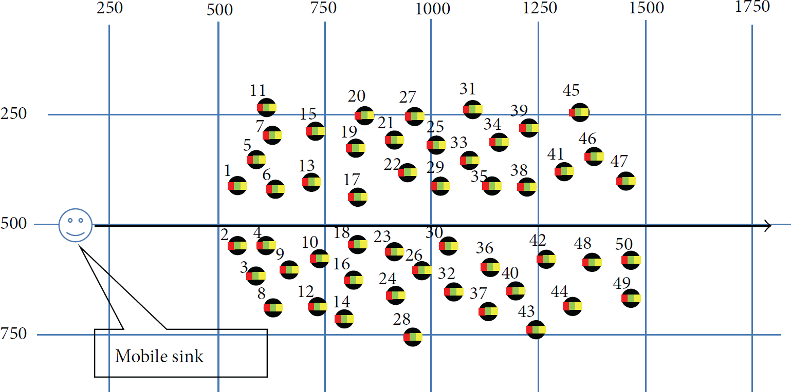
Deployment map.

Algorithm 1 describes the source code for calculating the received power used in the shadowing model. In our experiments, the received power is used for deciding the priority and allocating data transmission time.

Algorithm 1: Source code for calculating the received power.

Shadowing::Pr(Packet, Sender, Receiver) {

double L = getL();         //system loss

double lambda = getLambda();   //wavelength

double Xt, Yt, Zt;       //loc of transmitter

double Xr, Yr, Zr;       //loc of receiver

getLoc(Sender, &Xt, &Yt, &Zt);

getLoc(Receiver, &Xr, &Yr, &Zr);

double dX = Xr − Xt;

double dY = Yr − Yt;

double dZ = Zr − Zt;

double dist = sqrt(dX * dX + dY * dY + dZ * dZ);

double Pr;

//get antenna gain

double Gt = getAntenna()->getTxGain(dX, dY, dZ, lambda);

double Gr = getAntenna()->getRxGain(dX, dY, dZ, lambda);

//calculate receiving power at reference distance

double Pr0 = Friis(t->getTxPr(), Gt, Gr, lambda, L, dist0_);

//calculate average power loss predicted by path loss model

double avg_db = −10.0 * pathlossExp_ * log10(dist/dist0_);

//get power loss by adding a log-normal random variable (shadowing)

//the power loss is relative to that at reference distance dist0_

double powerLoss_db = avg_db + ranVar->normal(0.0, std_db_);

//calculate the receiving power at dist

Pr = Pr0 * pow(10.0, powerLoss_db/10.0);

return Pr;

}

5.2. Experiment Scheduling Policies

Based on the established experimental environment, we applied WFQ(T), WFQ(D), and PBRR scheduling policies besides the proposed CASF policy.

WFQ(T) (Weighted Fair Queuing by remaining time) is a packet-based scheduling policy that uses the remaining time of the sensor nodes in the mobile sink communication range as scheduling weight. The sensor node with the shortest remaining time has the highest priority. In addition, it performs rescheduling after the mobile sink receives a fixed quantity of data from a sensor node.

WFQ(D) (Weighted Fair Queuing by received data) performs packet-based scheduling according to the accumulated amount of data received from sensor nodes. It gives data transmission opportunity to the sensor nodes that transmitted the least amount of data to a mobile sink. However, since this policy does not consider the remaining time, the sensor nodes with the shortest remaining time cannot transmit sensing data.

PBRR (Packet-Based Round Robin) schedules data packets one by one from the data-receiving queues for the sensor nodes. In this policy, after the mobile sink receives a fixed quantity of data from a sensor node, the next sensor node has an opportunity in a round-robin fashion.

WFQ(T), WFQ(D), and PBRR perform rescheduling every one second, which is the period of data transmission. To analyze the data collection characteristics in these scheduling policies, we measured the number of received packets from each sensor node. To measure the effectiveness of data reception when communication errors occur, we measured the total number of received packets of each scheduling policy. In addition, to evaluate fair data collection of all scheduling policies, we calculated fairness indexes.

5.3. Experiment Results

5.3.1. Number of Packets of Sensor Nodes

Figure 11 shows the number of packets received in the mobile sink using the four scheduling policies. WFQ(T) shows a smaller number of received packets than other policies. In particular, sensor nodes 1 and 2 transmit 100 packets to mobile sink, which are whole data packets, but other sensor nodes cannot transmit any data packets. This difference is because sensor nodes 1 and 2 are the first sensor nodes the mobile sink meets, as shown in Figure 10. Before other sensor nodes connect to the mobile sink, sensor nodes 1 and 2 have several opportunities to transmit their data to the mobile sink. This condition resulted in unfair data reception in the mobile sink. WQF(T) uses only the remaining time of sensor nodes in the mobile sink communication range. It gives high priority to the sensor node with a short remaining time. However, the sensor nodes with short remaining time are usually located at a great distance from the mobile sink. The distance causes communication errors. Thus, even if the mobile sink preferentially requests data transmission to these sensor nodes, the quantities of data received from them are minor. Due to biased data transmissions and packet data losses in specific sensor nodes, WQF(T) did not support fair data transmission for the mobile sink.

Figure 11

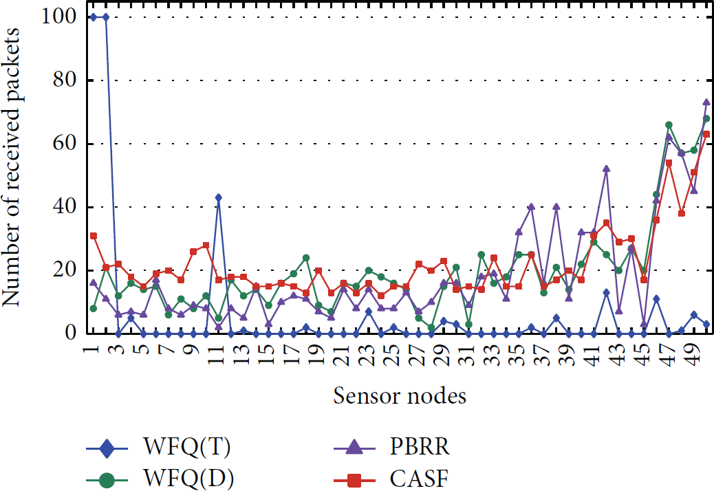
Number of received packets.

WFQ(D) does not show serious irregular data transmissions as WQF(T) did. However, particularly the 28th and 31st sensor nodes showed less data transmissions than other sensor nodes. The sensor node located in remote position from the routing path of the mobile sink has shorter communication time. Since WFQ(D) does not consider the communication time, these sensor nodes like the 28th and 31st sensor nodes have few chances to transmit their data.

PBRR schedules data collections from the sensor nodes in a round-robin style. The sensor nodes with the shortest remaining time in the mobile sink communication range have fewer opportunities to transmit data. For example, the 11th, 15th, and 45th sensor nodes are the corresponding sensor nodes. Since this policy does not use the accumulated amount of received data as a scheduling weight, the sensor nodes with more data transmission opportunities can be rescheduled again. This characteristic causes multiple data transmissions in specific sensor nodes. The 36th, 38th, and 42nd sensor nodes are those corresponding sensor nodes.

In CASF, most sensor nodes transmitted over 15 data packets. When deciding the priority orders, since CASF prefers the sensor nodes with many communication errors, sensor nodes located at a long distance have opportunities to transmit their data. The sensor nodes that issued low communication errors have shorter communication time, but the sensor nodes that issued high communication errors have longer communication time, proportionally. In addition, since the amounts of received data from each sensor node use scheduling weight when deciding the priority orders, multiple data transmissions from some sensor nodes do not occur. This characteristic supports a fair data collection scheduling between deployed sensor nodes.

5.3.2. Total Number of Received Packets

Figure 12 shows the total number of data packets received in the mobile sink. In WFQ(T), the mobile sink preferentially receives data packets from the sensor nodes located a long distance away. It received only 300 data packets. In WFQ(D) and PBRR policies, the mobile sink received more data packets as compared to the WFQ(T) policy. In Figure 12, these policies transmitted 993 data packets and 914 data packets individually. They did not adaptively treat the sensor nodes which have low or high opportunities in data transmissions.

Figure 12

Number of received data packet.

CASF allows the sensor nodes with low opportunity in data transmission to allocate over a long communication period. Otherwise, as the sensor nodes with a low communication error rate have a short communication period, they have enough opportunities for data transmission. For its effort, CASF makes the mobile sink fairly receive data packets from all sensor nodes. Thus, the total number of received data packets in wireless senor networks also increases. In Figure 12, CASF marked 1104 data packets, which is the maximum number among the scheduling policies. CASF showed 12% and 20% more received data packets than WFQ(D) and PBRR. From this result, we confirmed that CASF is a more effective data collection policy compared to other policies.

5.3.3. Fairness Index

To evaluate the degree of fairness in the data collection process, we use the fairness index as described in (5). The $x_i$ is the number of data packets transmitted from each sensor node, and the n is the number of sensor nodes:

$$\begin{array}{cc}& \mathrm{F}\mathrm{a}\mathrm{i}\mathrm{r}\mathrm{n}\mathrm{e}\mathrm{s}\hspace{0.17em}\hspace{0.17em}\mathrm{I}\mathrm{n}\mathrm{d}\mathrm{e}\mathrm{x}=\frac{{\left(\sum x_i\right)}^{\mathrm{2}}}{n\sum x_i^{\mathrm{2}}}.\end{array}$$

(5)

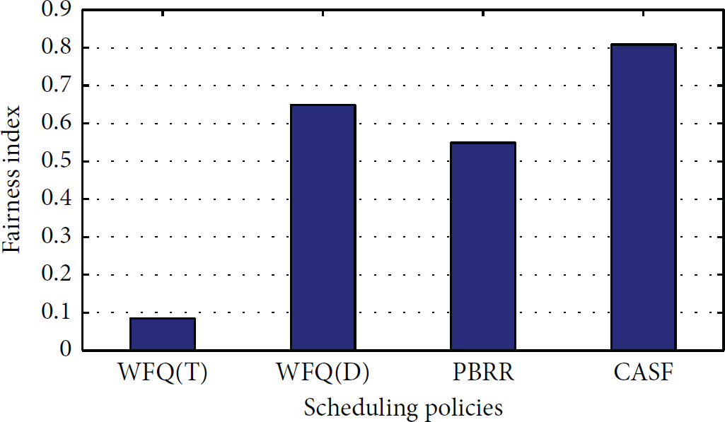
Figure 13 shows the result of the fairness index on experimented scheduling policies. In this figure, WFQ(T), WQF(D), PBRR, and CASF have 0.085, 0.65, 0.55, and 0.81 values individually. In particular, WFQ(T) showed an extremely low value compared to other policies. This result comes from the results shown in Figures 11 and 12. WFQ(T) had a low value regarding the total number of received data packets, and some sensor nodes transmitted all their data packets, while other sensor nodes did not transmit any data packets to the mobile sink. Since WFQ(D) uses the accumulated amount of received data as scheduling weight, multiple data transmissions did not occur. The fairness index of WFQ(D) is higher than those of WFQ(T) and PBRR. However, it did not consider the sensor nodes having short communication time. Thus, the fairness index of CASF is 24.6% higher than that of WQF(D). From this result, we can confirm that CASF has the best fairness value among experimented data collection scheduling policies.

Figure 13

Fairness index.

6. Conclusion and Future Works

When a mobile sink is applied to wireless sensor networks, fair data collection from the deployed sensor nodes is an important requirement. Since the mobile sink moves, the communication range of the mobile sink changes constantly. This variation causes the mobile sink to perform differential data collection between deployed sensor nodes. To address this problem, this paper proposed the CASF policy to support fair data collection in wireless sensor networks with a mobile sink. This concept is based on the communication error rates of sensor nodes and the accumulated amounts of data received from each sensor node.

In our experiments, we evaluated four data collection scheduling policies, including WFQ(T), WFQ(D), PBRR, and CASF. We analyzed the measured results according to the given performance metrics. WQF(T) allowed multiple data transmissions to specific sensor nodes. The WQF(D) and PBRR did not consider the characteristic of a mobile sink, which gives rise to many variations in the data transmission process. Thus, the sensor nodes located a long distance from a mobile sink could not fully transmit their sensing data. The three scheduling policies except CASF did not correspond to varied operational conditions. As a result, in the total number of received data packets, the CASF took 12% and 20% more received data packets compared to WFQ(D) and PBRR individually. In regard to the fairness index, CASF had about 24.6% and 47.3% improved performance compared to WFQ(D) and PBRR policies. From these results, we confirmed that CASF provided the best fair data collections for a mobile sink in wireless sensor networks.

In our future work, we will study an adaptive data collection scheduling policy when the routing path and speed of a mobile sink are varied, and the activities of mobile sinks occur in multiple hops.